Sampling and Reconstruction Jointly Optimized Model Unfolding Network for Single-Pixel Imaging

Abstract

In recent years, extensive research has shown that deep learning-based compressed image reconstruction algorithms can achieve faster and better high-quality reconstruction for single-pixel imaging, and that reconstruction quality can be further improved by joint optimization of sampling and reconstruction. However, these network-based models mostly adopt end-to-end learning, and their structures are not interpretable. In this paper, we propose SRMU-Net, a sampling and reconstruction jointly optimized model unfolding network. A fully connected layer or a large convolutional layer that simulates compressed reconstruction is added to the compressed reconstruction network, which is composed of multiple cascaded iterative shrinkage thresholding algorithm (ISTA) unfolding iteration blocks. To achieve joint optimization of sampling and reconstruction, a specially designed network structure is proposed so that the sampling matrix can be input into ISTA unfolding iteration blocks as a learnable parameter. We have shown that the proposed network outperforms the existing algorithms by extensive simulations and experiments.

1. Introduction

Single-pixel imaging (SPI), like computational ghost imaging, can achieve two-dimensional imaging using a single-pixel detector without spatial resolution, and is expected to provide a cost-effective solution for imaging in special wavelengths such as infrared and terahertz [1,2]. A single-pixel detector without spatial resolution is a point detector, also known as bucket detector. Unlike linear array detectors and area array detectors that contain multiple pixel units, single-pixel detectors have only one detection unit. As point detectors count all the photons collected, the pixel position cannot be obtained. In addition, since single-pixel detectors in the SPI system can simultaneously collect the light intensity from multiple pixels, they can obtain a higher signal-to-noise ratio [3,4]. Therefore, SPI has broad application prospects [5,6,7,8,9] in the fields of hyperspectral imaging [10,11,12], biological imaging [13,14,15], fluorescence lifetime imaging [16,17], and terahertz imaging [2].

However, SPI is time-consuming. Achieving fast and high-quality image reconstruction at a low sampling rate has always been one of the research goals for SPI. SPI, based on the compressed sensing (CS) theory, consists of two closely related steps: compressive sampling and image reconstruction. Three methods have been developed for compressive sampling and image reconstruction in the SPI system: The first method is to use a random Gaussian matrix or a fixed orthogonal matrix for the compressive sampling, and then reconstruct the image based on the CS theory [18,19]. In this method, the image is reconstructed by mining the prior information of the imaging scene under the condition that the sampling times are much lower than the number of pixels. The reconstruction algorithms include OMP [20], TVAL3 [21], ISTA [22], BCS [23], etc. Since the number of samples is much smaller than the number of image pixels, it is necessary to solve the uncertainty problem to reconstruct the image, which requires a long reconstruction time and a high computational complexity [24,25,26]. The second method also uses a random Gaussian matrix or fixed orthogonal matrix for the compressive sampling, followed by a deep learning-based reconstruction network for the image reconstruction [27,28,29,30,31,32,33,34,35,36,37,38,39]. After training, the reconstruction network with fixed weights maps low-dimensional sampled values to high-dimensional images, which can avoid the many computations caused by traditional iterative algorithms and thus complete the image reconstruction in a relatively short time. In 2017, Lyu et al. proposed a new computational ghost imaging framework based on deep learning (GIDL). The GIDL uses three hidden layers and one output layer to achieve image reconstruction with better performance at very low sampling rates [27]. In 2018, He et al. proposed a convolutional neural network for ghost imaging [28]. In 2019, Wang et al. proposed a one-step end-to-end neural network that directly uses the measured bucket signals to recover images [29]. In 2020, Li et al. proposed a deep image reconstruction network (Bsr2-Net) for SPI. Their network contains a fully connected layer and four Res2Net blocks, which achieves better results than the traditional algorithm TVAL3 [30]. Zhu et al. proposed a Y-net consisting of two encoders and one decoder, which works well under both deterministic and indeterministic lighting [31]. In 2021, Shang et al. proposed a two-step training TST-DL framework for computational imaging without physical priors, independent of an accurate representation of the imaging physics [32]. In 2022, Wang et al. proposed an end-to-end generative adversarial network (EGAN) to recover 2D image approximations from very low sampling rates [33]. These studies demonstrate that deep learning-based SPI enables faster, higher-quality image reconstruction. The third is to use deep learning to simultaneously optimize compressed sampling and image reconstruction [40,41,42,43,44,45,46,47]. In 2020, Li et al. proposed a sampling and reconstruction integrated convolutional neural network HRSC-Net for SPI [40]. In 2021, Gao et al. proposed a generative-model-based compressive reconstruction network optimized via sampling and transfer learning (OGTM), where the convergence speed and imaging quality of the network are significantly improved [41]. In 2022, Wang et al. proposed a physics-enhanced deep learning method for SPI. The method consists of three parts: encoding patterns, a differential ghost imaging (DGI) algorithm, and a deep neural network (DNN) model. Both the DNN model and the encoding patterns are trained and optimized [42]. These studies show that the reconstruction quality of images can be further improved with joint optimization of sampling and reconstruction using deep learning. However, most of the algorithms use an end-to-end learning network. The network is comparable to a “black box” as the network structure is not interpretable and there is a generalization issue in practical applications.

The model unfolding network, which unfolds each iteration step of the traditional algorithm into a network, has both interpretability and good reconstruction performance. It has been applied in compression reconstruction, super-resolution, image denoising, and so on [48,49,50]. We applied ISTA to our network to make our network interpretable, unlike the end-to-end network, which is like a black box, and to achieve better reconstruction quality. In order to obtain a better reconstruction performance at a low sampling rate for SPI, we added a sampling network to the deep unfolding network to achieve joint optimization of both sampling and reconstruction. Our contributions are summarized as follows:

• We propose a sampling and reconstruction jointly optimized model unfolding network (SRMU-Net) for the SPI system. To achieve joint optimization of both sampling and reconstruction, a specially designed network is proposed so that the sampling matrix can be input into each iteration block as a learnable parameter.
• We added a preliminary reconstruction loss term with a regularization parameter to the loss function of SRMU-Net, which can achieve a higher imaging accuracy and faster convergence.
• Extensive simulation experiments demonstrate that the proposed network, SRMU-Net, outperforms existing algorithms. By training the sampling layer to be binary, our designed network can be directly used in the SPI system, which we have verified by experiments.

2. Related Work and Background

2.1. ISTA

In SPI, based on CS, the imaging process can be denoted in Equation (1):

$$y=\Phi x+w,$$

(1)

where $x\in R^m$ is the object image, $y\in R^n$ is the measurement values. $\Phi \in R^{n*m}(n<<m)$ is the measurement matrix, and w represents noise.

In SPI, the number of measurements n is much smaller than the number of image pixels m. The reconstruction x via $y$ is the solution of the under-determined problem. Traditional CS reconstruction algorithms combine the prior knowledge of the scene to solve the under-determined problem. The prior knowledge includes sparsity priors, non-local low-rank regularization, and total variation regularization.

Based on the sparse prior, using the l₁ norm as the regularization term, the solution of x can be expressed by Equation (2):

$$x=\underset{x}{\min }\frac{1}{2}||\Phi x-y|{|}_2^2+\lambda ||x|{|}_1,$$

(2)

If x is sparse under transformation matrix $\psi$. The solution is shown in Equation (3):

$$x=\underset{x}{\min }\frac{1}{2}||\Phi x-y|{|}_2^2+\lambda ||\psi x|{|}_1,$$

(3)

This is the classic LASSO (least absolute shrinkage and selection operator) problem. Many researchers solve Equation (3) using gradient-based methods. Among the many gradient-based algorithms, the iterative shrinking threshold algorithm (ISTA) is a very interesting algorithm. ISTA updates x through a shrinking soft threshold operation in each iteration. It solves Equation (3) through two iterative steps, shown by Equations (4) and (5) [22]:

$$r^{(k)}=x^{(k-1)}-\rho {\Phi }^T(\Phi x^{(k-1)}-y),$$

(4)

$$x^{(k)}=\underset{x}{\arg \min }\frac{1}{2}||x-r^{(k)}|{|}_2^2+\lambda ||\psi x|{|}_1,$$

(5)

where k is the number of iterations, ρ is the iteration step size, Φ^T is the transpose of the sampling matrix, and λ is the regularization parameter. Equation (5) is a special case of proximal mapping, which can be solved by Equation (6):

$$x^{(k)}=W^{T}soft(W{r}^{(k)},\lambda ),$$

(6)

where W is a transformation matrix, $soft$ is a soft threshold function. ISTA usually requires many iterations to obtain satisfactory results, and the amount of calculation is large. The transformation matrix W and all parameters (ρ, λ) are predefined (i.e., do not change with k), which makes it difficult to adjust.

2.2. ISTA-Net and ISTA-Net+

In recent years, deep learning has made a series of breakthroughs in computer vision tasks such as image classification, super-resolution, object detection, and restoration [29]. Solving the inverse problem with deep neural networks has been extensively studied. Among them, reconstruction of compressed sampling images has become a recent research hotspot. One category is a purely data-driven approach, which employs end-to-end learning to map sampled values directly to target images without using any prior knowledge of the signal. R.G. Baraniuk et al. reconstructed compressed measurement images with stacked denoising autoencoders (SDA) [51]. ReconNet, proposed by Kuldeep et al., uses six convolutional layers to reconstruct a compressive image [52]. Based on ReconNet, Yao Hantao et al. proposed a block structure composed of three convolution and residual structures, and the DR2-Net from cascading four of such blocks. This network further improves the reconstruction result [53]. Inspired by the generative adversarial network (GAN), Bora et al. proposed using a pre-trained DCGAN for compressive reconstruction (CS-GM) [54]. These studies show that deep learning-based compressive reconstruction is faster and has a higher reconstruction accuracy than traditional model-driven algorithms. However, due to the purely data-driven approach, the network is treated as an end-to-end black box and its structure is not interpretable. The other category is a hybrid model-driven and data-driven approach that unfolds interpretable traditional reconstruction algorithms into a multi-layer neural network. The alternating direction method of multipliers (ADMM) is used to solve the decomposable convex optimization problem. By decomposing the objective function of the original problem into several solvable sub-problems, and then solving each sub-problem in parallel, the global solution of the original problem is obtained by coordinating the solution of the sub-problem. Yang et al. use two different solving methods to obtain two network structures, Basic-ADMM-Net and Generic-ADMM-Net, by model unfolding, which effectively improved the reconstruction speed and accuracy of the network [55]. Zhang et al. unfolded the ISTA into multi-layer neural networks, proposing ISTA-NET and ISTA-Net+ [56]. The specific method is as follows:

Two linear convolution operators separated by ReLU operators are used to replace the sparse transformation of ISTA, Equation (3) is transformed into Equation (7):

$$x=\underset{x}{\min }\frac{1}{2}||\Phi x-y|{|}_2^2+\lambda ||f(x)|{|}_1,$$

(7)

where f(·) is the sparse transformation space learned by the network. Equations (4)–(6) of the iterative steps are updated to Equations (8)–(10), ISTA is unfolding into the deep neural network, and the network is used to learn the iteration network parameters in each iteration block.

$$r^{(k)}=x^{(k-1)}-{\rho }^{(k-1)}{\Phi }^T(\Phi x^{(k-1)}-y),$$

(8)

$$x^{(k)}=\underset{x}{\arg \min }\frac{1}{2}||x-r^{\left(\mathrm{k}\right)}|{|}_2^2+\lambda ||f(x)|{|}_1,$$

(9)

$$x^{(k)}=F(soft(f(r^{(k)}),\lambda )),$$

(10)

where F(·) is the inverse process of f(·).

Based on ISTA-Net, ISTA-Net+ performs convolution on r^(k) of Equation (8) to extract the image features, and introduces a residual structure. ISTA-Net and ISTA-Net+ combine the advantages of traditional iterative algorithms and deep networks, and use a large amount of training data to optimize the step size, forward and reverse transformation matrices, and shrinkage thresholds. This improves the traditional iterative algorithm performance and endows the network with clear interpretability.

Although ISTA-Net and ISTA-Net+ achieve good compression-reconstruction performance, they use the hand-made sampling matrix for sampling and the least square method to realize the preliminary reconstruction. This limits some of their performance. We believe that there are two aspects that can be further improved, specifically for SPI. First, sampling and reconstruction can be jointly optimized. Unlike ISTA-Net and ISTA-Net+, which use the random Gaussian matrix for measurement, we abstracted the sampling process into a sampling sub-network of fully connected layers or large convolutional layers, which are cascaded with the reconstruction network for joint optimization to obtain the global optimal solution. Second, multiple loss terms are designed to make the network converge faster and achieve better performance.

3. Proposed Network

3.1. Network Architecture

Figure 1 shows the network structure diagram of SRMU-Net. The whole network consists of three subnetworks: a sampling subnetwork, a preliminary reconstruction subnetwork, and a deep reconstruction subnetwork. The sampling subnetwork and the preliminary reconstruction subnetwork are closely related, and constitute the structure of an encoder-decoder network. The sampling subnetwork was employed to simulate the compressive sampling of SPI. We designed two sampling methods: fully connected layer sampling and large convolutional layer sampling, which are described in detail in Section 3.2. The preliminary reconstruction subnetwork was used for low-quality image reconstruction. To reconstruct high-quality images, inspired by ISTA-net and ISTA-net+, we cascaded multiple ISTA iteration blocks into a deep reconstruction subnetwork. However, in contrast to ISTA-net and ISTA-net+, in order to achieve joint optimization of both sampling and reconstruction, we input the weight matrix of the sampling subnetwork as the measurement matrix Φ and measurement value $y$ into each iteration block together.

3.2. Sampling and Preliminary Reconstruction Subnetwork

The jointly optimized sampling and compressed reconstruction network mainly adopts a fully connected layer to simulate the compressed sampling. The fully connected layer weights after removing the bias and activation function replace the random Gaussian matrix as the measurement matrix. The number of the fully connected layer weights increases exponentially with the dimensionality of the reconstructed image. Compared with the fully connected layer, a large convolutional layer has the advantages of parameter sharing and sparse connection, which can greatly reduce the number of sampling layer weights. We compare the two sampling methods in Section 4.1.

3.2.1. Fully Connected Layer Sampling and Preliminary Reconstruction

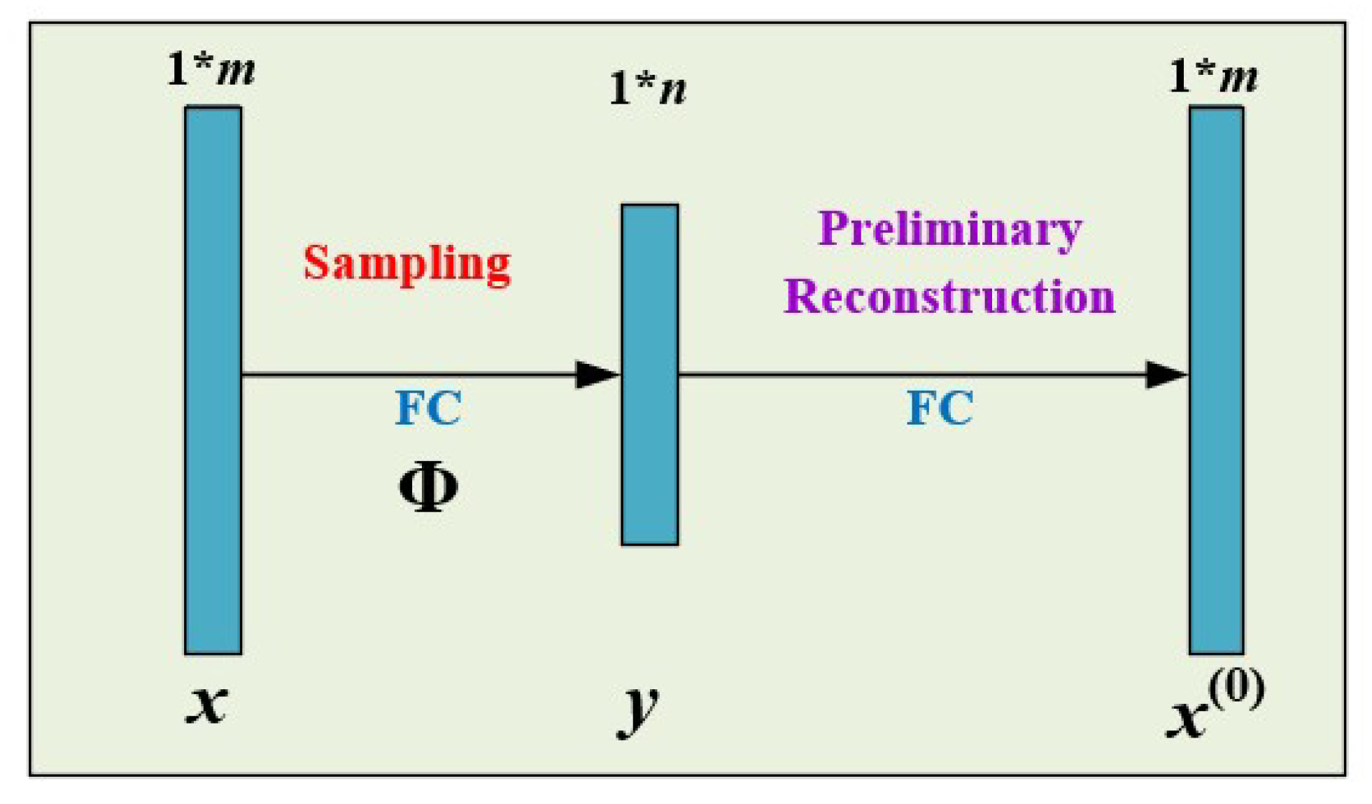
As shown in Figure 2, two fully connected layers form a sampling subnetwork and a preliminary reconstruction subnetwork, respectively. Original image input with a dimension of 32 × 32 is reshaped to a vector with a dimension of m = 1024, $x\in R^{1*m}$. The weight matrix $W_t\in R^{m*n}$ of the first fully connected layer can be thought of as a measurement matrix Φ, where n is related to the measurement rate. Therefore, the output value of the first fully connected layer can be considered as the measurement value $y\in R^{1*n}$, where n is the number of samples. The second fully connected layer maps the measurement value $y$ to the preliminary reconstructed image $x^{(0)}\in R^{1*m}$.

3.2.2. Large Convolutional Layer Sampling and Preliminary Reconstruction

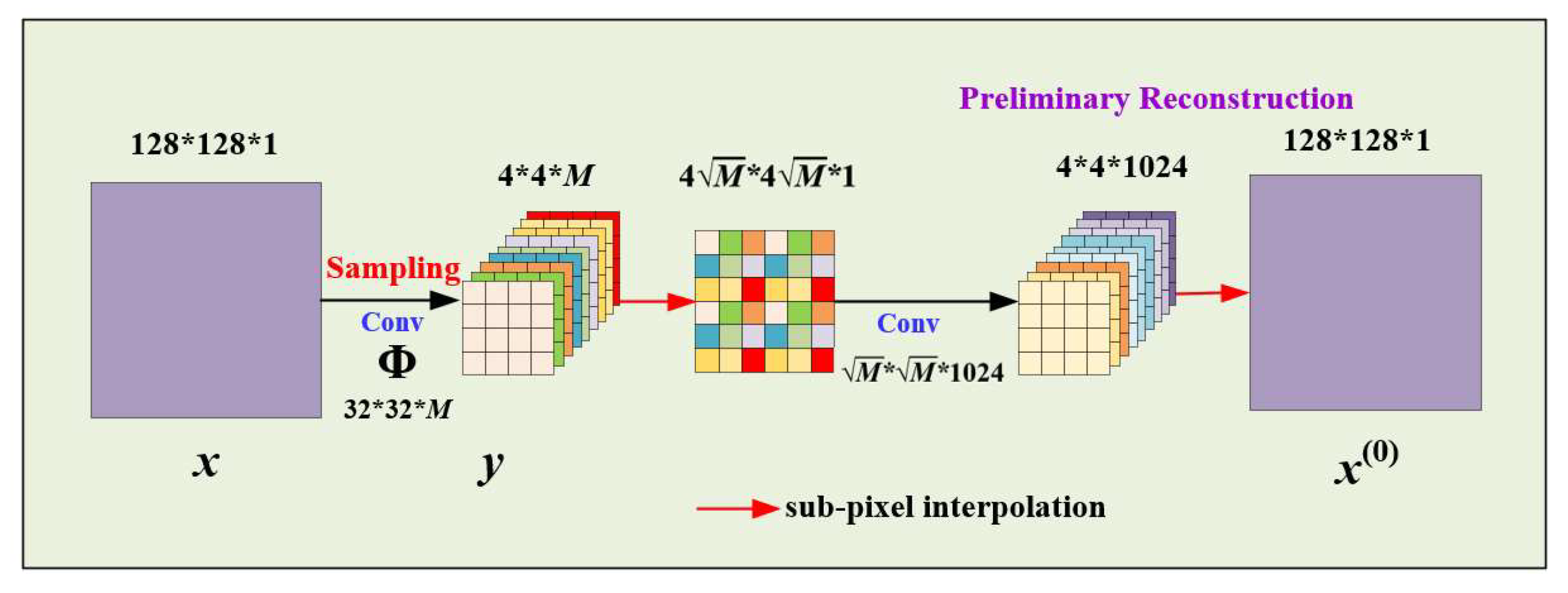
Figure 3 shows the structure diagram of a large convolutional layer sampling and preliminary reconstruction network. The dimension of the input image x is 128 × 128 × 1. The first convolutional layer of the network is the sampling layer, which consists of M convolution kernels, each with a size of 32 × 32 and a stride of 32. The sampling matrix can be expressed as $\Phi \in R^{32*32*M}$, where M is related to the measurement rate. The measurement value after sampling, which can be expressed as $y\in R^{4*4*M}$. $y$ is refactored a two-dimensional matrix with a size of $4\sqrt{M}\times 4\sqrt{M}\times 1$ by sub-pixel interpolation. The second convolutional layer of the network is the preliminary reconstruction layer, which consists of 1024 convolution kernels, each with a size of $\sqrt{M}\times \sqrt{M}$ and a stride of $\sqrt{M}$, and outputs the preliminary reconstruction result with a size of 4 × 4 × 1024. The preliminary reconstructed image $x^{(0)}\in R^{128*128*1}$ is obtained by sub-pixel interpolation. The first convolutional layer of the network is applied to the object for measurement. The measurement rate (MR) in terms of the number of convolution kernels M is given by $MR=\left(16*M\right)/\left(128*128\right)$. When the measurement rate is 25%, the number of parameters of the fully connected layer is 67108864, while that of the proposed large convolutional layer sampling method is 262144.

3.3. Deep Reconstruction Subnetwork

As shown in Figure 1, our deep reconstruction subnetwork is composed of five cascaded iteration blocks. According to Section 3.2, the output of the fully connected layer sampling and preliminary reconstruction is a one-dimensional vector, while the output of the large convolutional layer sampling and preliminary reconstruction is a two-dimensional matrix. Therefore, two different iteration block unfolding strategies are employed. For the fully connected layer sampling, the deep reconstruction subnetwork adopts a similar structure to the iteration block of ISTA-Net+. For the large convolutional layer sampling, we propose a new deep reconstruction network that extends to two-dimensional matrices.

3.3.1. The Iteration Block Based on Fully Connected Layer Sampling

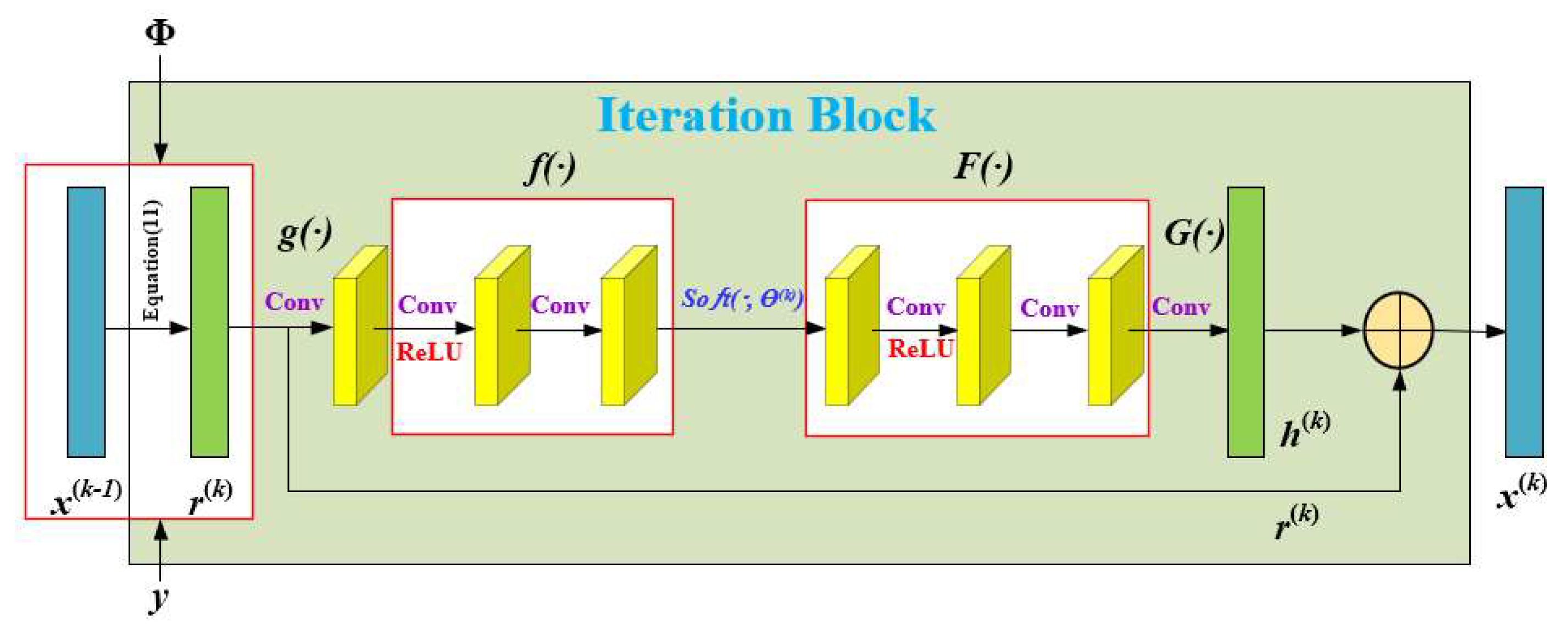
Figure 4 shows the iteration block based on fully connected layer sampling. From the upper network result $x^{(k-1)}\in R^{1*m},$$r^{(k-1)}\in R^{1*m}$ can be obtained following Equation (11). Unlike ISTA-net+, which uses a random Gaussian matrix as the measurement matrix Φ, we use the learnable weight matrix of the sampling sub-network as the measurement matrix Φ.

$$r^{(k)}=x^{(k-1)}-{\rho }^{(k-1)}{\Phi }^T(\Phi x^{(k-1)}-y),$$

(11)

r^(k) is reshaped to 32 × 32 × 1. Iteration blocks extract the feature maps of r^(k) by the first convolutional layer with 32 filters (size 3 × 3) and the process is denoted by g(·). The feature maps are mapped to the transform domain through transform operation. The transform operation denoted by f(·), consists of two linear convolution operators separated bya ReLU operator. A $soft$ function is used on the sparsely transformed data. F(·) denotes the process going from the transform domain back to the feature maps via two linear convolution operators separated by a ReLU operator. Each linear convolution consists of 32 convolution kernels, each with a size of 3 × 3. $h^{(k-1)}\in R^{32*32*1}$ is obtained by the last convolutional layer with 1 filter (size 3 × 3), this process is denoted by G(·). h^(k) is reshaped to 1 × m. A residual structure is used to combine r^(k) and h^(k) to get x^(k). This process is defined by Equations (12) and (13):

$$x^{(k)}=r^{(k)}+h^{(k)},$$

(12)

$$x^{(k)}=r^{(k)}+G(F(soft(f(g(r^{(k)})),{\theta }^{(k)}))),$$

(13)

where f(·) and F(·) are a pair of positive and inverse transformations, so the network needs to constrain $f\cdot F=I$. Inspired by the residual, we consider that r^(k) is the low-frequency part of the reconstructed image and h^(k) is the high-frequency part of the image that r^(k) cannot capture. The parameters in the nonlinear mapping and gradient descent can be learned through the end-to-end training of the network, and the learnable parameter set is $\{\Phi ,{\rho }^{(k)},{\theta }^{(k)},g^{(k)},G^{(k)},f^{(k)},F^{(k)}\}$.

3.3.2. The Iteration Block Based on Large Convolutional Layer Sampling

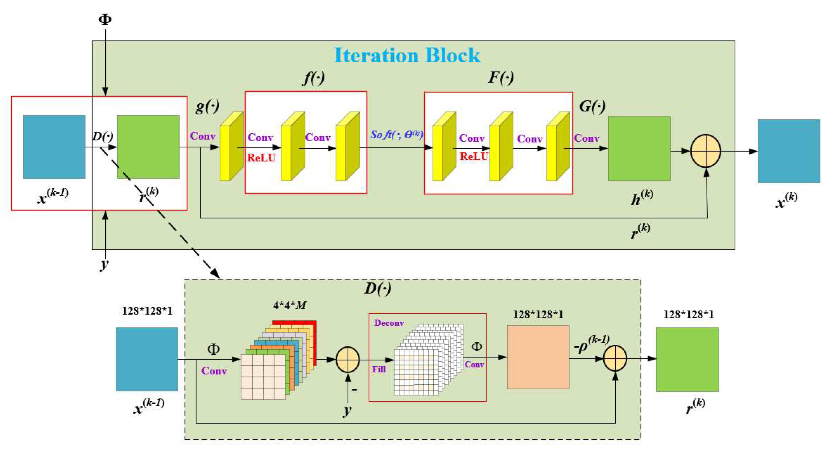
Figure 5 shows the iteration block based on large convolutional layer sampling. The dimension of the input is 128 × 128 × 1. As convolution is used for sampling, the measurement value is not in a one-dimensional vector. Therefore, r^(k) cannot be calculated directly with Equation (11). In Equation (11), $\Phi x^{(k-1)}$ can be thought of as a sampling operation, ${\Phi }^T(x^{(k-1)}-y)$ can be considered as an inverse sampling operation. For the measurement matrix of the large convolution sampling to be input into the iterative block as a learnable parameter, we especially designed the network structure denoted as D(·). Convolution and deconvolution are used to replace the sampling operation and inverse sampling operation in Equation (11). $x^{(k-1)}\in R^{128*128*1}$ is convolved with Φ, then subtracts the measurement value $y$. The value after subtraction is deconvolved with Φ. The deconvolution operation fills the matrix that is being convolved, then uses a 32 × 32 × M convolutional filter and a stride of 1 to restore the matrix dimension to 128 × 128 × 1. The result after deconvolution is multiplied by $-{\rho }^{(k-1)}$ and then added to x^(k−1) to get $r^{(k)}\in R^{128*128*1}$. We can transform Equation (11) into Equation (14):

$$r^{(k)}=D(x^{(k-1)})=x^{(k-1)}-{\rho }^{(k-1)}\Phi \tilde{\ast }(\Phi \ast x^{(k-1)}-y),$$

(14)

where $\tilde{\ast }$ represents a deconvolution operation, and $\ast$ represents a convolution operation. r^(k) is obtained by Equation (14). Except for the different data dimensions, the subsequent operations of the iteration block are consistent with Section 3.3.1. This process can be represented by Equations (12) and (13).

3.4. Loss Function

For SRMU-Net to better learn the related parameters, we designed a loss function that adapts to this network. Given a training dataset ${\{(x_i,x_i)\}}_{i=1}^{N_b}$, the loss function is shown in Equation (15). It consists of three items: the final reconstruction loss δ_d, the sparse transformation loss δ_c, and the preliminary reconstruction loss δ_s. δ_d is the mean square error of the final reconstruction result $x_i^{(K)}$ and $x_i$. To ensure the constraint conditions $f^{(k)}\cdot F^{(k)}=I$ is statisfied, δ_c is the mean square error of $F^{(k)}(f^{(k)}(x_i))$ and $x_i$. To obtain better reconstruction results and evaluate the sampling subnetwork, δ_s is the mean square error of the preliminary reconstruction results $x_i^{(0)}$ and $x_i$.

$$\delta ={\delta }_d+\alpha {\delta }_c+\beta {\delta }_s$$

(15)

where: $\left\{\begin{array}{l}{\delta }_d=\frac{1}{N{N}_b}{\displaystyle {\sum }_{i=1}^N||x_i^{(K)}}-x_i|{|}_2^2\\ {\delta }_c=\frac{1}{N{N}_b}{\displaystyle {\sum }_{i=1}^N{\displaystyle {\sum }_{k=1}^K||F^{(k)}(f^{(k)}(x_i))}}-x_i|{|}_2^2\\ {\delta }_s=\frac{1}{N{N}_b}{\displaystyle {\sum }_{i=1}^N||x_i^{(0)}}-x_i|{|}_2^2\end{array}\right.$, $K$, $N_b$, $N$ is the number of iteration block, the total number of image block in the dataset, and the size of each image block, respectively. α and β are regularization parameters, in our experiments, α is set to 0.01, and we a numerical discussion on β is provided in Section 4.2.

4. Results and Discussion

In this section, we describe the processing of the image training data and the training-related parameters. We used the same 91 images in [51] to construct the training set. For the fully connected layer sampling, N_b = 22,227, N = 1024, and the pixel blocks size is 32 × 32. For the large convolutional layer sampling, N_b = 7789, N = 16,384, and the pixel blocks size was 128 × 128. We trained the model at four different measurement rates: {1.5%, 5%, 10%, 25%}. Our network was implemented with TensorFlow. The training settings were as follows: learning rate = 0.0001, number of epochs = 1000, batch size = 32, and optimized by an Adam optimizer. The loss function in Section 3.4 was used to optimize the network. For testing, we sampled eight images of size 256 × 256 from the set11 [55] dataset. Peak signal-to-noise ratio (PSNR) and structural similarity (SSIM) were used to quantitatively evaluate the reconstruction results.

4.1. Comparison of Different Sampling Methods

We compared the two sampling methods designed in this paper (i.e., SRMU-Net based on fully connected layer sampling in Section 3.2.1, and SRMU-Net based on large convolutional layer sampling in Section 3.2.2) with the random Gaussian matrix sampling method (ISTA-Net+). For testing, the large image was cropped into the small image required by the network, and the reconstruction was performed using block compressed sensing. The reconstructed small images were spliced back, and then PSNR was used to measure the effect of the reconstructed image. For a fair comparison, Equation (15) was used as the loss function and β was temporarily set to 0.

The comparisons in

Table 1. Test set performance comparison in terms of the average PSNR (dB) under different MR with different sampling methods. The best performance is marked in bold.

Sampling Methods	MR = 25%	MR = 10%	MR = 5%	MR = 1.5%
Fully connected layer sampling	33.09	28.41	25.85	21.87
Large convolutional layer Sampling	33.20	28.98	26.14	23.18
Random Gaussian matrix sampling	31.82	26.59	23.09	19.31

show that the two proposed sampling methods are superior to random Gaussian matrix sampling, which indicates that the measurement matrix of network optimization is superior to the random Gaussian matrix. As mentioned in the introduction, joint optimization of sampling and reconstruction can further improve image quality. Compared with fully connected layer sampling, large convolutional layer sampling achieves better results at MR = 1.5%, 5%, 10%, and 25%. The lower the sampling rate, the greater the gap. As large convolutional layer sampling has the advantages of parameter sharing and sparse connections, it has better information extraction performance at low MR. The subsequent simulation experiments used SRMU-Net based on large convolutional layer sampling.

4.2. Discussion on Different β Values of Loss Function

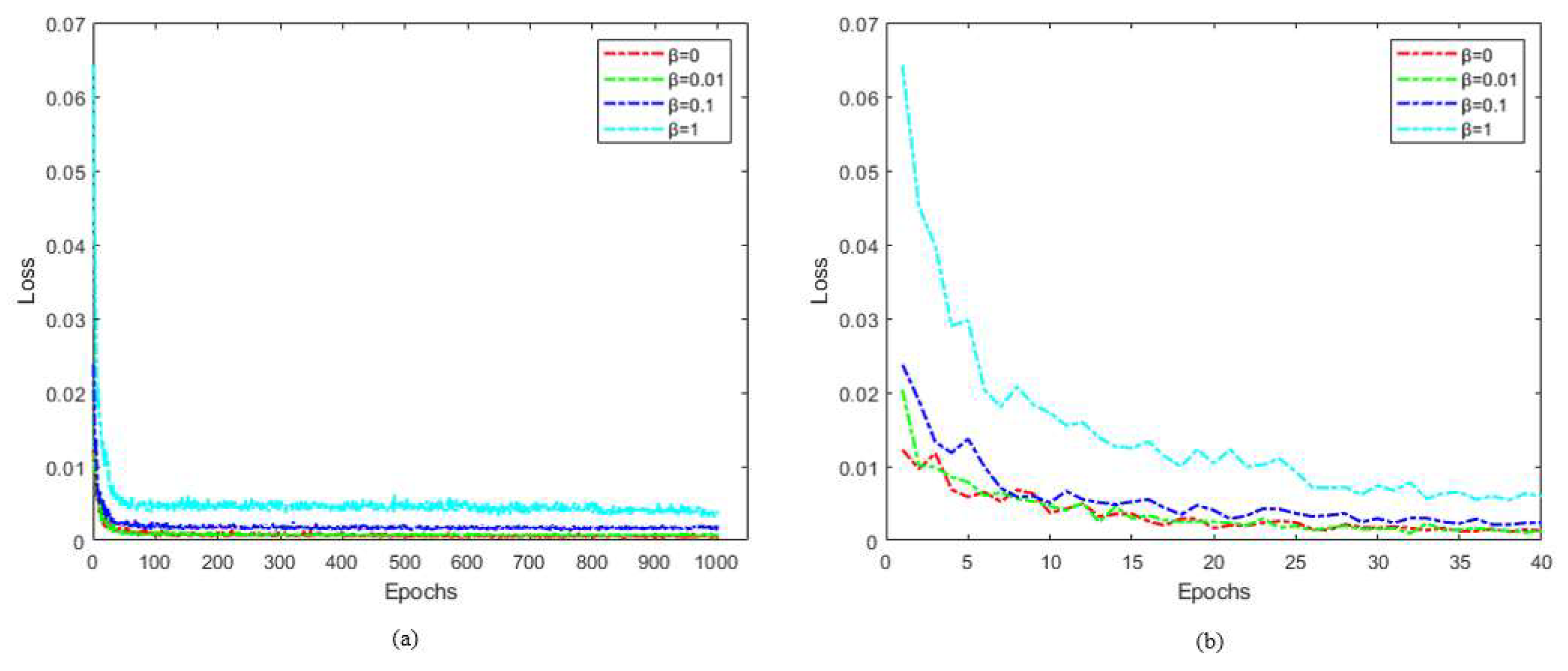
From Section 3.4, our loss function consists of three parts: the final reconstruction loss δ_d, the sparse transformation loss δ_c with a regularization parameter α, and the preliminary reconstruction loss δ_s with a regularization parameter β. This section discusses the value of regularization parameter β. For testing, image processing is the same as in Section 4.1. Keeping other network parameters the same, we compared the network’s performance when the measurement rate was 1.5%, 5%, 10%, 25% and the β value was 0, 0.01, 0.1, 1. We also explored the network convergence with a measurement rate of 25% for β values of 0, 0.01, 0.1, 1.

In

Table 2. Test set performance comparison in terms of the average PSNR (dB) with different β values under different MR. The best performances are marked in bold.

β Value	MR = 25%	MR = 10%	MR = 5%	MR = 1.5%
β = 0	33.20	28.98	26.14	23.15
β = 0.01	33.89	29.21	26.49	23.12
β = 0.1	33.66	29.10	26.67	23.05
β = 1	32.83	28.74	26.50	23.17

, the PSNR of the reconstruction results with different β values at MR = 1.5%, 5%, 10% and 25% are compared. The results prove that adding a loss term for the sampling and reconstruction subnetwork is effective. Network performance of β = 0.01, 0.1, and 1 was better than that β = 0 at MR = 5% and 10%. Different β values resulted in similar performance at MR = 1.5%. At MR = 25% and 10%, the reconstruction with β = 1 was poor. For the different β values, Figure 6a shows the overall convergence process at MR = 25%, and Figure 6b shows the convergence process from 0 to 40 epochs at MR = 25%. According to Table 2, the best reconstruction result was achieved for β = 0.01 at MR = 25%, while the loss of the network converged rapidly in the early stage of training and finally stabilized at a low value. This indicates that adding a preliminary reconstruction error term with a regularization parameter to the loss function can achieve better reconstruction performance and faster convergence. When β = 0.01, the network reconstruction results were best at MR = 25% and 10%, and slightly worse at MR = 5% and 1.5%. Therefore, we set the β of the loss function to 0.01.

4.3. Comparison with Existing Algorithms

In this section, we design a series of comparative experiments to evaluate SRMU-Net. We also compare our network with an optimization-based traditional reconstruction algorithm, TVAL3, and two popular network-based deep compressive sensing reconstruction algorithms, ISTA-Net+ and DR2-Net. TVAL3 is a reconstruction algorithm based on total variational regularization [21]. The algorithm only needs the sampling matrix and the corresponding measurement values to restore the original image. DR2-Net uses a sampling matrix for sampling, then a full connected layer for preliminary reconstruction, and finally, four blocks for the deep reconstruction required to restore the image [53]. Each block is composed of three convolution layers and a residual structure. These three algorithms use the random Gaussian matrix for sampling. To ensure fairness of comparison, we used the same 91 images, optimizer, learning rate, epoch, and batch size when training ISTA-Net+ and DR2-Net. For testing, image processing is the same as in Section 4.1. We used PSNR and SSIM to evaluate reconstruction performance on the test set.

Table 3. Comparison of different algorithms’ test set performances under different MRs in terms of PSNR (dB) and SSIM. The best performance is marked in bold.

Image Name	Methods	MR = 25%		MR = 10%		MR = 5%		MR = 1.5%
		PSNR/dB	SSIM	PSNR/dB	SSIM	PSNR/dB	SSIM	PSNR/dB	SSIM
Barbara	TVAL3	24.07	0.72	21.76	0.55	20.45	0.46	16.80	0.32
	DR2-Net	25.30	0.80	22.81	0.63	21.72	0.54	19.72	0.44
	ISTA-Net+	27.27	0.86	23.08	0.67	21.44	0.56	19.60	0.42
	SRMU-Net	29.25	0.90	24.35	0.72	23.74	0.66	22.47	0.54
Boats	TVAL3	28.59	0.83	24.09	0.66	21.09	0.53	17.83	0.40
	DR2-Net	30.52	0.87	26.24	0.75	23.17	0.62	20.04	0.48
	ISTA-Net+	32.55	0.91	26.79	0.78	23.05	0.63	19.40	0.45
	SRMU-Net	35.06	0.95	29.69	0.87	26.67	0.77	23.14	0.60
Cameraman	TVAL3	25.83	0.82	21.67	0.67	19.55	0.57	16.37	0.46
	DR2-Net	25.71	0.82	22.56	0.72	20.72	0.63	18.18	0.53
	ISTA-Net+	27.33	0.86	22.93	0.72	20.34	0.63	17.62	0.50
	SRMU-Net	29.51	0.90	25.64	0.82	23.57	0.75	21.28	0.65
Foreman	TVAL3	34.82	0.91	29.26	0.81	24.76	0.69	20.03	0.56
	DR2-Net	35.36	0.92	31.70	0.87	28.41	0.81	23.93	0.70
	ISTA-Net+	38.18	0.95	33.10	0.89	29.16	0.83	23.61	0.69
	SRMU-Net	39.43	0.97	35.59	0.93	32.59	0.89	28.23	0.81
House	TVAL3	31.75	0.86	26.37	0.75	23.16	0.64	19.41	0.54
	DR2-Net	33.26	0.87	29.07	0.80	25.75	0.73	22.21	0.63
	ISTA-Net+	35.34	0.90	30.02	0.82	26.09	0.75	20.84	0.60
	SRMU-Net	36.85	0.92	32.64	0.87	29.80	0.82	24.88	0.71
Monarch	TVAL3	27.39	0.86	20.93	0.65	18.02	0.52	14.96	0.37
	DR2-Net	28.55	0.90	23.36	0.78	20.33	0.64	16.76	0.46
	ISTA-Net+	31.67	0.94	24.86	0.81	19.99	0.65	15.80	0.43
	SRMU-Net	33.93	0.97	28.33	0.91	24.37	0.82	19.57	0.61
Parrot	TVAL3	26.87	0.86	23.26	0.75	21.07	0.65	14.43	0.44
	DR2-Net	28.71	0.89	24.66	0.82	22.47	0.75	19.97	0.64
	ISTA-Net+	29.29	0.92	25.37	0.84	22.05	0.76	19.36	0.63
	SRMU-Net	32.70	0.95	28.57	0.90	25.63	0.84	23.18	0.75
Peppers	TVAL3	29.47	0.85	22.95	0.68	19.68	0.54	15.13	0.38
	DR2-Net	29.73	0.86	25.09	0.76	21.98	0.64	18.52	0.51
	ISTA-Net+	32.94	0.91	26.55	0.80	22.62	0.69	18.22	0.49
	SRMU-Net	34.22	0.94	28.91	0.89	25.59	0.83	22.21	0.69
Mean	TVAL3	28.60	0.84	23.79	0.69	20.97	0.58	16.87	0.43
	DR2-Net	29.64	0.87	25.69	0.77	23.07	0.68	19.92	0.55
	ISTA-Net+	31.82	0.91	26.59	0.79	23.09	0.69	19.31	0.53
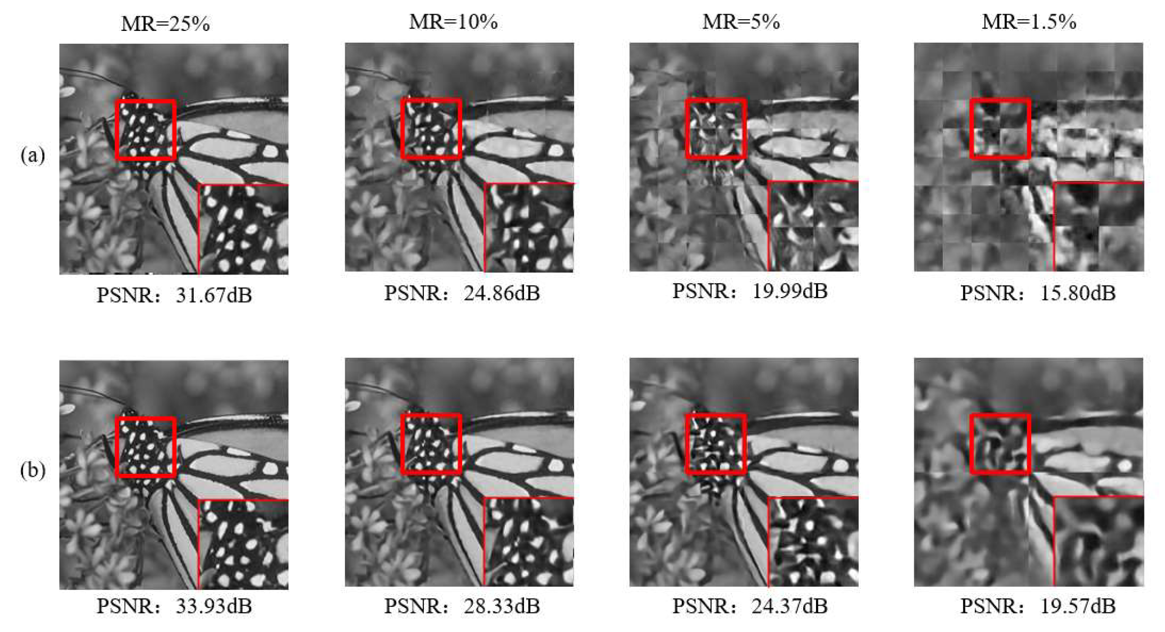
	SRMU-Net	33.89	0.94	29.21	0.86	26.49	0.80	23.12	0.67

and Figure 7 show the reconstruction results of different algorithms at different MRs on the test set. The results show that the network-based deep reconstruction algorithm is better than the optimization-based traditional reconstruction algorithm. At all MRs, the proposed SRMU-Net achieves the best performance. The lower the measurement rate, the more obvious the advantages. For example: at MR = 1.5%, SRMU-Net is 3.2dB better than DR2-Net. At MR = 25%, SRMU-Net is 2.05dB better than ISTA-Net+. Experiments show that SRMU-Net outperforms other reconstruction algorithms. Figure 7 shows the reconstruction results of SRMU-Net and ISTA-Net+ at all MRs. Since the “Monarch” is sized 256 × 256, it is divided into 4 subimages sized 128 × 128 for SRMU-Net, and 64 subimages sized 32 × 32 for ISTA-Net+. The proposed SRMU-Net is able to reconstruct more details and sharper edges.

4.4. Imaging Results of SRMU-Net on SPI System

We built an SPI system in the early stage [57]. To use the network to verify the performance of this system, the first layer of the network needs to be trained with binary weights. It is loaded onto the digital micromirror array to achieve efficient compressed sampling. Meanwhile, the hyperparameters of the network and the training data set remain unchanged. The binarization method and the corresponding training method are introduced in our previous paper [56]. From the previous three sections, it is clear that SRMU-Net based on large convolutional sampling achieves better reconstruction results. Therefore, this section compares it with the mainstream reconstruction algorithm TVAL3. To ensure fairness of comparison, we used a binary random Gaussian measurement matrix for testing TVAL3. We imaged the object “turntable” at four MRs in the SPI system and reconstructed the image using different algorithms. The reconstructed image dimension was 128 × 128. An image with a size of 128 × 128 is divided into 16 subimages sized 32 × 32 when using TVAL3. Figure 8 shows the imaging results of SRMU-Net and TVAL3 at different MRs. SRMU-Net achieves higher PSNR than TVAL3. Compared with the results of TVAL3, the images reconstructed with SRMU-Net show more image details. This is consistent with the previous numerical simulation results.

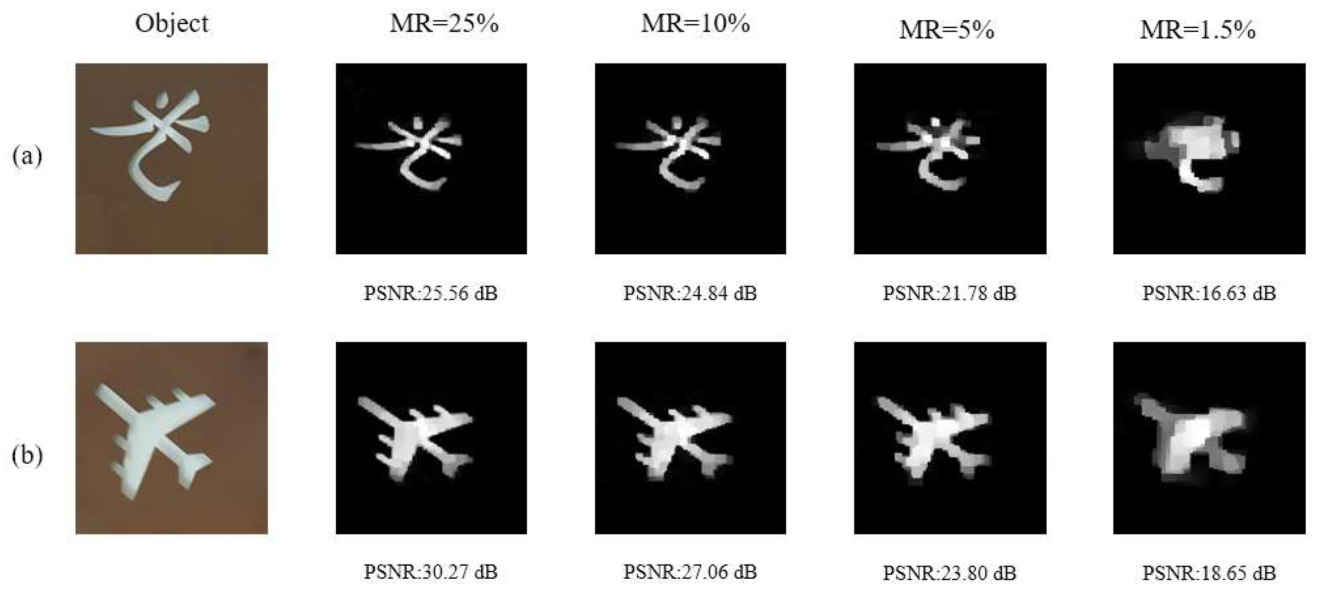
To verify the performance of SRMU-Net, different objects are selected for imaging in this paper. As shown in Figure 9, we imaged the Chinese Word for “light” and the pattern of “airplane”. We found that SRMU-Net could not reconstruct clear images at MR = 1.5%, while it could reconstruct clear images in other cases. This proves that the network proposed in this paper can be used to reconstruct different objects, and has broad prospects in specialist fields such as medical diagnosis, astronomical observation, spectral measurement, etc.

5. Conclusions

This paper proposes a sampling and reconstruction jointly optimized model unfolding network (SRMU-Net) for the SPI system. Two types of layers, a fully connected layer and a large convolutional layer, which simulate compressive sampling, are added to ISTA unfolding iteration blocks. To achieve joint optimization of both sampling and reconstruction, the weight matrix of the sampling layer is input into each iteration block as a learnable parameter. The results from the simulation experiments show that large convolutional layer sampling can not only reduce the number of weights but also obtain better reconstruction quality. This advantage becomes more obvious when the measurement rate is low. Adding a preliminary reconstruction loss term to the loss function of the network leads to faster convergence and better reconstruction. Extensive experiments demonstrate that the proposed network SRMU-Net outperforms existing algorithms. The lower the measurement rate, the more obvious the advantage. By training the sampling layer to be binary, SRMU-Net can be applied to the SPI system.

References

1. Komiyama, S.; Astafiev, O.; Antonov, V.; Kutsuwa, T.; Hirai, H. A single-photon detector in the far-infrared range. Nature 2000, 403, 405–407. [Google Scholar] [CrossRef]
2. Komiyama, S. Single-photon detectors in the terahertz range. IEEE J. Sel. Top. Quantum Electron. 2010, 17, 54–66. [Google Scholar] [CrossRef]
3. Gabet, R.; Stéphan, G.-M.; Bondiou, M.; Besnard, P.; Kilper, D. Ultrahigh sensitivity detector for coherent light: The laser. Opt. Commun. 2000, 185, 109–114. [Google Scholar] [CrossRef]
4. Sobolewski, R.; Verevkin, A.; Gol’Tsman, G.-N.; Lipatov, A.; Wilsher, K. Ultrafast superconducting single-photon optical detectors and their applications. IEEE Trans. Appl. Supercond. 2003, 13, 1151–1157. [Google Scholar] [CrossRef]
5. Zhao, C.; Gong, W.; Chen, M.; Li, E.; Wang, H.; Xu, W.; Han, S. Ghost imaging lidar via sparsity constraint. Appl. Phys. Lett. 2012, 101, 141123. [Google Scholar] [CrossRef] [Green Version]
6. Gong, W.; Han, S. High-resolution far-field ghost imaging via sparsity constraint. Sci. Rep. 2015, 5, 9280. [Google Scholar] [CrossRef] [Green Version]
7. Sun, B.; Edgar, M.-P.; Bowman, R.; Vittert, L.-E.; Welsh, S.; Bowman, A.; Padgett, M.-J. 3D computational imaging with single-pixel detectors. Science 2013, 340, 844–847. [Google Scholar] [CrossRef] [PubMed] [Green Version]
8. Yu, W.-K.; Yao, X.-R.; Liu, X.-F.; Li, L.-Z.; Zhai, G.-J. Three-dimensional single-pixel compressive reflectivity imaging based on complementary modulation. Appl. Opt. 2015, 54, 363–367. [Google Scholar] [CrossRef]
9. Wang, X.-G.; Lin, S.-S.; Xue, J.-D.; Xu, B.; Chen, J.-L. Information security scheme using deep learning-assisted single-pixel imaging and orthogonal coding. Opt. Express 2023, 31, 2402–2413. [Google Scholar] [CrossRef]
10. Sinclair, M.-B.; Haaland, D.-M.; Timlin, J.-A.; Jones, H.-D. Hyperspectral confocal microscope. Appl. Opt. 2006, 45, 6283–6291. [Google Scholar] [CrossRef]
11. Pian, Q.; Yao, R.; Sinsuebphon, N.; Intes, X. Compressive hyperspectral time-resolved wide-field fluorescence lifetime imaging. Nat. Photonics 2017, 11, 411–414. [Google Scholar] [CrossRef] [Green Version]
12. Rock, W.; Bonn, M.; Parekh, S.-H. Near shot-noise limited hyperspectral stimulated Raman scattering spectroscopy using low energy lasers and a fast CMOS array. Opt. Express 2013, 21, 15113–15120. [Google Scholar] [CrossRef] [PubMed]
13. Fredenberg, E.; Hemmendorff, M.; Cederström, B.; Åslund, M.; Danielsson, M. Contrast-enhanced spectral mammography with a photon-counting detector. Med. Phys. 2010, 37, 2017–2029. [Google Scholar] [CrossRef] [PubMed]
14. Symons, R.; Krauss, B.; Sahbaee, P.; Cork, T.-E.; Lakshmanan, M.-N.; Bluemke, D.-A.; Pourmorteza, A. Photon-counting CT for simultaneous imaging of multiple contrast agents in the abdomen: An in vivo study. Med. Phys. 2017, 44, 5120–5127. [Google Scholar] [CrossRef] [Green Version]
15. Yu, Z.; Leng, S.; Jorgensen, S.-M.; Li, Z.; Gutjahr, R.; Chen, B.; McCollough, C.-H. Evaluation of conventional imaging performance in a research whole-body CT system with a photon-counting detector array. Phys. Med. Biol. 2016, 61, 1572. [Google Scholar] [CrossRef] [PubMed] [Green Version]
16. Becker, W.; Bergmann, A.; Hink, M.-A.; König, K.; Benndorf, K.; Biskup, C. Fluorescence lifetime imaging by time-correlated single-photon counting. Microsc. Res. Tech. 2004, 63, 58–66. [Google Scholar] [CrossRef] [PubMed]
17. Duncan, R.-R.; Bergmann, A.; Cousin, M.-A.; Apps, D.-K.; Shipston, M.-J. Multi-dimensional time-correlated single photon counting (TCSPC) fluorescence lifetime imaging microscopy (FLIM) to detect FRET in cells. J. Microsc. 2004, 215, 1–12. [Google Scholar] [CrossRef] [Green Version]
18. Gribonval, R.; Chardon, G.; Daudet, L. Blind calibration for compressed sensing by convex optimization. In Proceedings of the 2012 IEEE International Conference on Acoustics, Speech and Signal Processing (ICASSP), Kyoto, Japan, 25–30 March 2012; pp. 2713–2716. [Google Scholar]
19. Do, T.-T.; Gan, L.; Nguyen, N.; Tran, T.-D. Sparsity adaptive matching pursuit algorithm for practical compressed sensing. In Proceedings of the 2008 42nd Asilomar Conference on Signals, Systems and Computers, Pacific Grove, CA, USA, 26–29 October 2008; pp. 581–587. [Google Scholar]
20. Tropp, J.A.; Gilbert, A.-C. Signal recovery from random measurements via orthogonal matching pursuit. IEEE Trans. Inf. Theory 2007, 53, 4655–4666. [Google Scholar] [CrossRef] [Green Version]
21. Li, C. An Efficient Algorithm for Total Variation Regularization with Applications to the Single Pixel Camera and Compressive Sensing. Master’s Thesis, Rice University, Houston, TX, USA, 2010. [Google Scholar]
22. Beck, A.; Teboulle, M. A fast iterative shrinkage-thresholding algorithm for linear inverse problems. SIAM J. Imaging Sci. 2009, 2, 183–202. [Google Scholar] [CrossRef] [Green Version]
23. Ji, S.; Xue, Y.; Carin, L. Bayesian compressive sensing. IEEE Trans. Signal Process. 2008, 56, 2346–2356. [Google Scholar] [CrossRef]
24. Candès, E.-J.; Romberg, J.; Tao, T. Robust uncertainty principles: Exact signal reconstruction from highly incomplete frequency information. IEEE Trans. Inf. Theory 2006, 52, 489–509. [Google Scholar] [CrossRef] [Green Version]
25. Li, C.; Yin, W.; Jiang, H.; Zhang, Y. An efficient augmented Lagrangian method with applications to total variation minimization. Comput. Optim. Appl. 2013, 56, 507–530. [Google Scholar] [CrossRef] [Green Version]
26. Kim, Y.; Nadar, M.S.; Bilgin, A. Compressed sensing using a Gaussian Scale Mixtures model in wavelet domain. In Proceedings of the 2010 IEEE International Conference on Image Processing, Hong Kong, China, 26–29 September 2010; pp. 3365–3368. [Google Scholar]
27. Lyu, M.; Wang, W.; Wang, H.; Wang, H.; Li, G.; Chen, N.; Situ, G. Deep-learning-based ghost imaging. Sci. Rep. 2017, 7, 17865. [Google Scholar] [CrossRef] [PubMed] [Green Version]
28. He, Y.; Wang, G.; Dong, G.; Zhu, S.; Chen, H.; Zhang, A.; Xu, Z. Ghost imaging based on deep learning. Sci. Rep. 2018, 8, 6469. [Google Scholar] [CrossRef] [Green Version]
29. Wang, F.; Wang, H.; Wang, H.; Li, G.; Situ, G. Learning from simulation: An end-to-end deep-learning approach for computational ghost imaging. Opt. Express 2019, 27, 25560–25572. [Google Scholar] [CrossRef]
30. Li, B.; Yan, Q.-R.; Wang, Y.-F.; Yang, Y.-B.; Wang, Y.-H. A binary sampling Res2net reconstruction network for single-pixel imaging. Rev. Sci. Instrum. 2020, 91, 033709. [Google Scholar] [CrossRef]
31. Zhu, R.; Yu, H.; Tan, Z.; Lu, R.; Han, S.; Huang, Z.; Wang, J. Ghost imaging based on Y-net: A dynamic coding and decoding approach. Opt. Express 2020, 28, 17556–17569. [Google Scholar] [CrossRef] [PubMed]
32. Shang, R.; Hoffer-Hawlik, K.; Wang, F.; Situ, G.; Luke, G. Two-step training deep learning framework for computational imaging without physics priors. Opt. Express 2021, 29, 15239–15254. [Google Scholar] [CrossRef]
33. Wang, X.; Zhu, A.; Lin, S.; Xu, B. Learning-based high-quality image recovery from 1D signals obtained by single-pixel imaging. Opt. Commun. 2022, 521, 128571. [Google Scholar] [CrossRef]
34. Zhu, Y.L.; She, R.-B.; Liu, W.-Q.; Lu, Y.-F.; Li, G.-Y. Deep Learning Optimized Terahertz Single-Pixel Imaging. IEEE Trans. Terahertz Sci. Technol. 2021, 12, 165–172. [Google Scholar] [CrossRef]
35. Rizvi, S.; Cao, J.; Hao, Q. Deep learning based projector defocus compensation in single-pixel imaging. Opt. Express 2020, 28, 25134–25148. [Google Scholar] [CrossRef]
36. Woo, B.H.; Tham, M.-L.; Chua, S.-Y. Deep Learning Based Single Pixel Imaging Using Coarse-to-Fine Sampling. In Proceedings of the 2022 IEEE 18th International Colloquium on Signal Processing & Applications (CSPA), Selangor, Malaysia, 12 May 2022; pp. 127–131. [Google Scholar]
37. Shang, R.; O’Brien, M.-A.; Luke, G.-P. Deep-learning-driven Reliable Single-pixel Imaging with Uncertainty Approximation. arXiv 2021, arXiv:2107.11678. [Google Scholar]
38. Karim, N.; Rahnavard, N. SPI-GAN: Towards single-pixel imaging through generative adversarial network. arXiv 2021, arXiv:2107.01330. [Google Scholar]
39. Yang, Z.; Bai, Y.-M.; Sun, L.-D.; Huang, K.-X.; Liu, J.; Ruan, D.; Li, J.-L. SP-ILC: Concurrent Single-Pixel Imaging. Object Location, and Classification by Deep Learning. Photonics 2021, 8, 400. [Google Scholar] [CrossRef]
40. Li, W.-C.; Yan, Q.-R.; Guan, Y.-Q.; Yang, S.-T.; Peng, C.; Fang, Z.-Y. Deep-learning-based single-photon-counting compressive imaging via jointly trained subpixel convolution sampling. Appl. Opt. 2020, 59, 6828–6837. [Google Scholar] [CrossRef] [PubMed]
41. Gao, W.; Yan, Q.-R.; Zhou, H.-L.; Yang, S.-T.; Fang, Z.-Y.; Wang, Y.-H. Single photon counting compressive imaging using a generative model optimized via sampling and transfer learning. Opt. Express 2021, 29, 5552–5566. [Google Scholar] [CrossRef] [PubMed]
42. Wang, F.; Wang, C.; Deng, C.; Han, S.; Situ, G. Single-pixel imaging using physics enhanced deep learning. Photonics Res. 2022, 10, 104–110. [Google Scholar] [CrossRef]
43. Sun, S.; Yan, Q.; Zheng, Y.; Wei, Z.; Lin, J.; Cai, Y. Single pixel imaging based on generative adversarial network optimized with multiple prior information. IEEE Photonics J. 2022, 14, 4. [Google Scholar] [CrossRef]
44. Lin, J.; Yan, Q.; Lu, S.; Zheng, Y.; Sun, S.; Wei, Z. A Compressed Reconstruction Network Combining Deep Image Prior and Autoencoding Priors for Single-Pixel Imaging. Photonics 2022, 9, 343. [Google Scholar] [CrossRef]
45. Hoshi, I.; Shimobaba, T.; Kakue, T.; Ito, T. Single-pixel imaging using a recurrent neural network combined with convolutional layers. Opt. Express 2020, 28, 34069–34078. [Google Scholar] [CrossRef]
46. Peng, Y.; Tan, H.; Liu, Y.; Zhang, M. Structure Prior Guided Deep Network for Compressive Sensing Image Reconstruction from Big Data. In Proceedings of the 2020 6th International Conference on Big Data and Information Analytics (BigDIA), Shenzhen, China, 4–6 December 2020; pp. 270–277. [Google Scholar]
47. Shi, W.; Jiang, F.; Liu, S.; Zhao, D. Image compressed sensing using convolutional neural network. IEEE Trans. Image Process. 2019, 29, 375–388. [Google Scholar] [CrossRef] [PubMed]
48. Zheng, S.; Yang, X.; Yuan, X. Two-Stage is Enough: A Concise Deep Unfolding Reconstruction Network for Flexible Video Compressive Sensing. arXiv 2022, arXiv:2201.05810. [Google Scholar]
49. Zhang, K.; Gool, L.-V.; Timofte, R. Deep unfolding network for image super-resolution. In Proceedings of the IEEE/CVF Conference on Computer Vision and Pattern Recognition, Seattle, WA, USA, 13–19 June 2020; pp. 3217–3226. [Google Scholar]
50. Yin, H.; Wang, T. Deep side group sparse coding network for image denoising. IET Image Process. 2022, 17, 1–11. [Google Scholar] [CrossRef]
51. Mousavi, A.; Patel, A.-B.; Baraniuk, R.-G. A deep learning approach to structured signal recovery. In Proceedings of the 2015 53rd Annual Allerton Conference on Communication, Control, and Computing (Allerton), Monticello, IL, USA, 29 September–2 October 2015; pp. 1336–1343. [Google Scholar]
52. Kulkarni, K.; Lohit, S.; Turaga, P.; Kerviche, R.; Ashok, A. Reconnet: Non-iterative reconstruction of images from compressively sensed measurements. In Proceedings of the IEEE Conference on Computer Vision and Pattern Recognition (CVPR), Las Vegas, NV, USA, 27–30 June 2016; pp. 449–458. [Google Scholar]
53. Yao, H.; Dai, F.; Zhang, S.; Zhang, Y.; Tian, Q.; Xu, C. Dr2-net: Deep residual reconstruction network for image compressive sensing. Neurocomputing 2019, 359, 483–493. [Google Scholar] [CrossRef] [Green Version]
54. Bora, A.; Jalal, A.; Price, E.; Dimakis, A.-G. Compressed sensing using generative models. In Proceedings of the International Conference on Machine Learning, Sydney, Australia, 6–11 August 2017; pp. 537–546. [Google Scholar]
55. Sun, J.; Li, H.; Xu, Z. Deep ADMM-Net for compressive sensing MRI. Adv. Neural Inf. Process. Syst. 2016, 19, 10–18. [Google Scholar]
56. Zhang, J.; Ghanem, B. ISTA-Net: Interpretable optimization-inspired deep network for image compressive sensing. In Proceedings of the IEEE Conference on Computer Vision and Pattern Recognition (CVPR), Salt Lake City, UT, USA, 18–23 June 2018; pp. 1828–1837. [Google Scholar]
57. Guan, Y.; Yan, Q.; Yang, S.; Li, B.; Cao, Q.; Fang, Z. Single photon counting compressive imaging based on a sampling and reconstruction integrated deep network. Opt. Commun. 2020, 459, 124923. [Google Scholar] [CrossRef]
Figure 1. The network structure diagram of SRMU-Net, which consists of three subnetworks.
Photonics 10 00232 g001
Figure 2. Structure diagram of a fully connected layer sampling and preliminary reconstruction network.
Photonics 10 00232 g002
Figure 3. Structure diagram of a large convolutional layer sampling and preliminary reconstruction network.
Photonics 10 00232 g003
Figure 4. Structure diagram of the iteration block based on fully connected layer sampling.
Photonics 10 00232 g004
Figure 5. Structure diagram of the iteration block based on large convolutional layer sampling. D(·) is a specially designed network structure that enables the measurement matrix to be input into the iteration blocks as a learnable parameter.
Photonics 10 00232 g005
Figure 6. Loss curves of different β values (MR = 25%). (a) From the full training process. (b) In the 0–40 epoch range.
Photonics 10 00232 g006
Figure 7. Reconstruction results using ISTA-Net+ and SRMU-Net. (a) Reconstructed by ISTA-Net+. (b) Reconstructed by SRMU-Net.
Photonics 10 00232 g007
Figure 8. Single-pixel imaging results using the traditional method and the proposed method. (a) The reconstruction algorithm is TVAL3. (b) The reconstruction algorithm is SRMU-Net.
Photonics 10 00232 g008
Figure 9. Single-pixel imaging results of other objects using SRMU-Net. (a) “light” pattern reconstruction results. (b) “airplane” pattern reconstruction results.
Photonics 10 00232 g009