Perfect Invisibility Modes in Dielectric Nanofibers

Abstract

With the help of the original mathematical method for solving Maxwell’s equations, it is shown that in dielectric waveguides along with usual waveguides and quasi-normal modes, there are perfect invisibility modes or perfect non-scattering modes. In contrast to the usual waveguide modes, at eigenfrequencies of the perfect invisibility modes, light can propagate in free space. The properties of the invisibility modes in waveguides of circular and elliptical cross-sections are analyzed in detail. It is shown that at the eigenfrequencies of the perfect invisibility modes, the power of the light scattered from the waveguide tends to zero and the optical fiber becomes invisible. The found modes can be used to create highly sensitive nanosensors and other optical nanodevices, where radiation and scattering losses should be minimal.

1. Introduction

Recently, invisible objects and related devices were discussed widely in the world scientific community. The active development of metamaterial technology has provoked a new burst of interest for invisibility and cloaking in science and technics [1,2,3,4,5,6,7,8,9,10].

To achieve perfect invisibility, the object must not reflect the electromagnetic wave back and not absorb or scatter it in side and forward directions. In terms of the theory of light scattering, this means that in the perfect case, the total scattering cross-section should be equal to zero.

Due to the rapid development of new areas of physics, such as the physics of metamaterials [1,2,3,4,5,6,7,8,9,10], transformation optics [11,12,13,14,15,16,17,18], and plasmonics [19,20], it has become possible to create cloaking coatings that significantly reduce the scattering of incident electromagnetic radiation by an object.

At the present time, among the variety of cloaking concepts, the following most developed principles should be distinguished:

(1)

cloaking based on the wave flow phenomenon (transformation optics) [11,12,13,14,15,16,17,18];

(2)

cloaking based on scattering compensation [21,22,23,24];

(3)

active cloaking [25,26];

(4)

external cloaking [27,28].

The manifestations of invisibility mentioned above are “artificial” in the sense that they are achieved through artificially created material structures. In this work, we propose an alternative formulation of the invisibility concept. Namely, for each dielectric object, we propose to find such configurations of electromagnetic fields, with the structure allowing one to place a given object into this field without any scattering. In other words, to demonstrate the “new” invisibility, we propose to find such solutions of sourceless Maxwell’s equations in the presence of a dielectric body that decreases at infinity and does not have radiation losses. Since such statement of the problem does not imply the presence of electric or magnetic currents at infinity, such solutions can be referred to as eigenmodes.

Usual waveguide modes in dielectric waveguides (see, e.g., [29]) also propagate without radiation losses, but their existence is possible only when the propagation constant h is greater than the wavenumber in vacuum (h > k₀), so that the wave propagation in free space is impossible at frequencies of waveguide modes.

Quasi-normal modes in dielectric bodies are found by solving the sourceless Maxwell equations with the Sommerfeld radiation conditions at infinity [30], and therefore such modes are fundamentally related to radiation losses. Moreover, such modes increase unlimited at infinity, requiring the development of very complex artificial approaches for their use (see, e.g., [31,32,33,34]).

However, finding all modes in dielectric bodies is a non-trivial task not only from a computational point of view, and therefore the waveguide and quasi-normal modes do not exhaust the entire set of modes that exist in dielectric bodies. Quite recently, in [35,36], it has been shown that in 3D dielectric nanoparticles of a finite volume, there can be an infinite number of perfect non-radiating modes that do not have radiation losses at all.

The goal of this work is to study the perfect invisibility modes in dielectric nanowaveguides rather than in 3D dielectric nanoparticles. In this article, we will consider solutions of Maxwell’s equations with a zero propagation constant (h = 0, exp(ihz) = 1), which distinguishes them from usual waveguide modes with h > k₀ radically and allows them to be excited by external fields propagating in free space. In this case, in contrast to the statement of problems for finding bound states in the continuum in planar waveguides [37,38,39], which assumes one or another periodic structure of waveguides, we will consider the usual smooth waveguides of an arbitrary cross-section. Supposing that the fields do not change along the waveguide, that is, in the case of a zero propagation constant (h = 0), we will show that in this experimentally simpler geometry, previously unknown perfect invisibility modes or, more specifically, perfect non-scattering modes, can exist. To find the perfect invisibility modes in waveguides, we will not use the Sommerfeld radiation conditions at infinity. Instead of this, to describe fields outside the waveguide, we use such solutions of Maxwell’s equations in free space that do not have singularities upon analytic continuation into the waveguide interior.

The plan for the rest of the work is as follows. Section 2 presents the general theory of the perfect invisibility modes in a waveguide of an arbitrary cross-section. Section 3.1 presents analytical solutions for the invisibility modes with TM polarization (PTM modes) in a circular waveguide and numerical experiments on light scattering from waveguides with Comsol Multiphysics, confirming the presence of deep minima in the scattered power at the frequencies of the perfect invisibility modes, which can be verified experimentally. Section 3.2 will present analytical solutions for the perfect invisibility TM polarized modes in a waveguide of an arbitrary elliptical cross-section and the results of numerical experiments on light scattering from waveguides with Comsol Multiphysics, confirming their practical importance. Section 3.3 presents an example of applying the found effects to create displacement nanosensors.

2. Materials and Methods

The geometry of the problem is shown in Figure 1. A dielectric waveguide has the permittivity ε, and its shape is characterized by the radius R in the case of a circular cross-section (see Section 3.1) and semi-axes a and b in the case of an elliptical cross-section. ξ and η denote elliptical coordinates (see Section 3.2).

We will say that the perfect invisibility mode with TM polarization (H_z(x,y) ≠ 0, E_z = 0) is excited in the waveguide if the outgoing wave

$$H_z^{out}={\displaystyle \sum _n{A}_n{H}_n^{\left(1\right)}\left(k_0\rho \right)e^{in\phi }}$$

(1)

exactly complements the incoming wave

$$H_z^{in}={\displaystyle \sum _n{A}_n{H}_n^{\left(2\right)}\left(k_0\rho \right)e^{in\phi }}$$

(2)

In (1) and (2) 0 < ρ < ∞, 0 < ϕ < 2π are the cylindrical coordinates, k₀ = ω/c is the wavenumber, in which ω is the frequency and c is the speed of light in vacuum, and A_n are the expansion coefficients in terms of cylindrical harmonics, which can be found from the boundary conditions at the surface of the nanofiber. It is assumed everywhere that time dependence has the form exp(-iω t). In (1) and (2) $H_n^{\left(1,2\right)}\left(k_0\rho \right)$ are the Hankel functions. Definitions and properties of the special functions used in this work can be found in [40].

Under conditions (1) and (2), the total magnetic field outside the waveguide will be equal to

$$H_z\left(\rho ,\phi ,\omega \right)=H_z^{in}+H_z^{out}=2{\displaystyle \sum _n{A}_n{J}_n\left(k_0\rho \right)e^{in\phi }},$$

(3)

where $J_n\left(k_0\rho \right)$ is the Bessel function.

Since (3) must be satisfied to ensure the absence of scattering or invisibility, then to find the perfect invisibility modes for an arbitrary waveguide, we propose to use solutions of the Maxwell equations outside the fiber in the form (3) instead of the usual Sommerfeld conditions [30]

$$H_z^S\left(\rho ,\phi ,\omega \right)={\displaystyle \sum _n{A}_n{H}_n^{\left(1\right)}\left(k_0\rho \right)e^{in\phi }}.$$

(4)

Obviously, if a solution of sourceless Maxwell’s equations with outside fields in the form (3) exists, then in principle, it does not have a flux of energy and radiation. Since (3) has no singularities in the entire space (including the waveguide interior), then finding modes in an unbounded space can be reduced to finding fields in the volume of the fiber only. As a result, the system of equations that uniquely determines the perfect invisibility modes in a dielectric waveguide with permittivity ε, can be written as a system of two equations for the strengths of two auxiliary electric fields E₁(x,y) and E₂(x,y)

$$\begin{array}{l}\nabla \times E_1=i{k}_0{H}_1,\hspace{1em}\nabla \times H_1=-i{k}_0\epsilon E_1,\hspace{1em}\mathrm{inside} \mathrm{waveguide},\\ \nabla \times E_2=i{k}_0{H}_2,\hspace{1em}\nabla \times H_2=-i{k}_0{E}_2,\hspace{1em}\mathrm{inside} \mathrm{waveguide},\\ n\times \left(E_1-E_2\right)=0,\hspace{1em}n\times \left(H_1-H_2\right)=0,\hspace{1em}\mathrm{at} \mathrm{the} \mathrm{boundary},\end{array}$$

(5)

where ∇ is the gradient operator, n is the unit vector normal to the boundary of a waveguide, H₁(x,y) and H₂(x,y) are corresponding magnetic field strengths. It is important to note that system (5) is self-sufficient and there is no need to impose any condition at infinity to solve it.

At some real values of the frequency or wavenumber k₀, the system of Equation (5) becomes consistent, i.e., the perfect invisibility modes arise. It is very important that, due to the specific structure of (5), there is nothing common between the frequencies of the perfect modes and the frequencies of the usual quasi-normal modes, which are obtained by using the Sommerfeld condition (4) at infinity. The modes found from (5) are orthogonal in the sense that

$${\displaystyle \underset{S}{\mathrm{\int }}dS\left(\epsilon E_{1,n}\cdot E_{1,m}-E_{2,n}\cdot E_{2,m}\right)}={\delta }_{nm},$$

(6)

where integration is over the cross-section of the waveguide S, and δ_nm is the Kronecker delta symbol. Condition (6) also differs significantly from the orthogonality conditions for the quasi-normal modes.

The physical (observable) fields inside the waveguide are determined by E₁ and H₁, while the physical (observable) fields outside the waveguide are defined by the analytic continuation of the E₂ and H₂ from the interior domain. The system of Equation (5) is very complicated and there is no rigorous mathematical theory for it in the general case. Nevertheless, the conditions for the existence of the perfect invisibility modes for an arbitrary elliptical waveguide will be presented below.

The definition of modes through the system of Equation (5) is a mathematical definition. However, both usual quasi-normal and perfect invisibility modes can be detected in scattering experiments as well. Therefore, in addition to (5), we also study the spectra of the scattered power P^scat and the energy stored in the waveguide W^stored. In this case, the deep minima of the scattering spectrum will indicate the excitation of the perfect invisibility modes, while the maxima in the stored energy spectrum will indicate the excitation of quasi-normal modes.

For a deeper understanding of the physics of perfect invisibility modes, it is of great importance to compare their eigen frequencies with the eigen frequencies of so-called confined modes [41] with a magnetic field different from zero only inside the waveguide. The electric field of the confined modes is zero everywhere. The confined modes can appear in the limit ε → ∞ and must satisfy the equations:

$$\begin{array}{l}\nabla \times \nabla \times H_n=K_n^2{H}_n, \mathrm{inside} \mathrm{waveguide}\\ H_n=0, \mathrm{at} \mathrm{the} \mathrm{boundary}\end{array}$$

(7)

A remarkable property of the confined modes is that their frequencies K_n do not depend on the permittivity ε. Eigenfrequencies in a vacuum, k_0,n, are related to the frequencies of the confined modes by the relation $K_n=\sqrt{\epsilon }{k}_{0,n}$. Finding the eigenfrequencies of the confined modes is much easier than finding the eigenfrequencies of the perfect invisibility modes. If the confined modes exist, then in the limit ε→∞ their frequencies can be close to the frequencies of perfect invisibility modes and usual quasi-normal modes, and therefore throughout the work, we will compare the frequencies of the perfect invisibility modes and the confined modes. To do this, the expression $k_{0}R\sqrt{\epsilon }$ will be used as the size parameter of the waveguide, where R is the effective radius of the waveguide.

We emphasize once again that in this work we consider solutions of Maxwell’s Equation (5), where the outside fields (3) are nonsingular with analytic continuation inside the waveguide. However, along with invisibility modes (3), (5) there are modes with outside fields that can be represented as an expansion in terms of Neumann functions N_n

$$H^N\left(\rho ,\phi ,\omega \right)={\displaystyle \sum _n{B}_n{N}_n\left(k_0\rho \right)e^{in\phi }},$$

(8)

where B_n are the coefficients that can be found from the boundary conditions at the waveguide surface.

External fields (8) have a singularity when they are analytically continued inside the waveguide and, therefore, the modes corresponding to them do not have the main property of the perfect invisibility modes found by us—the absence of scattering or invisibility, since scattering is large at their eigenfrequencies. Therefore, such solutions are not considered in this work.

Our results are very general and applicable within an arbitrary frequency range, where the waveguide permittivity can vary over a wide range. For example, Si has a permittivity ε = 12–16 in the visible and infrared ranges [42], PbTe has a permittivity ε = 36 in the infrared range [43], Bi₂Te₃ has exceptionally high permittivity ranging between 50 and 60 throughout the 2–10 μm region [44]. In the microwave frequency range, the permittivity varies even more widely. With this in mind, we built graphs for different values of permittivity.

3. Results

3.1. Perfect Invisibility Modes in a Waveguide with a Circular Cross-Section

The existence of perfect invisibility modes in a cylindrical waveguide is the easiest to prove in the case of a circular cross-section (Figure 1a).

In the case of TM polarization, the magnetic field has only one z-component, H_z, in the direction perpendicular to the waveguide cross-section. In this case, based on the complete system of Maxwell Equation (5), for H_z one can obtain the Helmholtz equation [45]

$$\begin{array}{l}\left(\frac{{\partial }^2}{\partial x^2}+\frac{{\partial }^2}{\partial y^2}+k_0^2\epsilon \right)H_{1,z}=0, \mathrm{inside} \mathrm{nanofiber},\\ \left(\frac{{\partial }^2}{\partial x^2}+\frac{{\partial }^2}{\partial y^2}+k_0^2\right)H_{2,z}=0, \mathrm{inside} \mathrm{nanofiber},\\ \left.\begin{array}{l}{H}_{1,z}=H_{2,z}\\ \left(n\cdot \nabla \right)H_{1,z}=\epsilon \left(n\cdot \nabla \right)H_{2,z}\end{array}\right\}, \mathrm{at} \mathrm{the} \mathrm{boundary},\end{array}$$

(9)

where ε is the permittivity of the waveguide. In the case under consideration, it is convenient to solve Equation (9) in the cylindrical coordinates. Inside the waveguide of the radius R, an arbitrary nonsingular solution has the form (the index m is the order of the mode):

$$H_z^{}=J_m\left(k_0\rho \sqrt{\epsilon }\right)e^{im\phi },\hspace{1em}\rho <R,$$

(10)

while outside the waveguide, an arbitrary nonsingular solution in the entire space has the form:

$$H_z=J_m\left(k_{0}R\sqrt{\epsilon }\right)\frac{J_m\left(k_0\rho \right)}{J_m\left(k_{0}R\right)}{e}^{im\phi },\hspace{1em}0<\rho <\infty .$$

(11)

By construction, (10) and (11) are continuous on the waveguide surface. The requirement for the continuity of the tangential component of the electric field, E_φ, leads to the dispersion equation

$$J_m\left(k_{0}R\sqrt{\epsilon }\right)=\frac{1}{\sqrt{\epsilon }}{J}_m\left(k_{0}R\right)\frac{J_m^{\prime }\left(k_{0}R\sqrt{\epsilon }\right)}{J_m^{\prime }\left(k_{0}R\right)},$$

(12)

where the prime next to the function means its derivative. This equation differs from the equation that defines the quasi-normal modes [45]

$$J_m\left(k_{0}R\sqrt{\epsilon }\right)=\frac{1}{\sqrt{\epsilon }}{H}_m^{\left(1\right)}\left(k_{0}R\right)\frac{J_m^{\prime }\left(k_{0}R\sqrt{\epsilon }\right)}{H_m^{\left(1\right)}{}^{\prime }\left(k_{0}R\right)}$$

(13)

by the Hankel functions replacement with the usual Bessel functions.

It is easy to see that Equation (12) as a function of k₀ definitely has an infinite number of real roots that determine the frequencies of the perfect invisibility modes. In this case, solutions (10), (11) are real functions.

Figure 2 shows H_z as a function of the radius for the quasi-normal (TM₁₁) and perfect invisibility (PTM₁₁) modes. The eigenfrequencies of these modes are found from the solution of Equations (12) and (13) for m = 1 and are equal to k₀R = 1.261 and k₀R = 1.051 − 0.07i respectively. From Figure 2 it follows that the perfect invisibility mode decreases at infinity. This fact radically distinguishes it from the usual quasi-normal mode, which increases without limit at infinity. For higher order modes (m = 2, 3, …) the situation is similar.

Figure 3 shows the dependence of the frequencies of the perfect invisibility modes $k_{0}R\sqrt{\epsilon }$ of TM type (PTM) in a cylindrical waveguide of circular cross-section on 1/ε.

It follows from Figure 3 that the frequency of the PTM₀₁ mode in the limit ε→∞ is determined by the root of the Bessel function $J_2\left(k_{0}R\sqrt{\epsilon }\right)=0$, and not by the root $J_0\left(k_{0}R\sqrt{\epsilon }\right)=0$, indicating that this mode, unlike the others, is not confined one [41]), that is, its field outside the waveguide does not vanish in this limit. Note that in the case of 3D axisymmetric particles, all TM and PTM modes are confined ones.

It is easy to see that the excitation of the nanofiber by a cylindrical wave proportional to (11) leads to zero scattered power, since the condition (12) corresponds to zero of the Mie scattering coefficient, a_m ([30] p. 199)

$$a_m=-\frac{\sqrt{\epsilon }{J}_m\left(k_{0}R\sqrt{\epsilon }\right)J_m^{\prime }\left(k_{0}R\right)-J_m\left(k_{0}R\right)J_m^{\prime }\left(k_{0}R\sqrt{\epsilon }\right)}{\sqrt{\epsilon }{J}_m\left(k_{0}R\sqrt{\epsilon }\right)H_m^{\left(1\right)}{}^{\prime }\left(k_{0}R\right)-H_m^{\left(1\right)}\left(k_{0}R\right)J_m^{\prime }\left(k_{0}R\sqrt{\epsilon }\right)}.$$

(14)

Indeed, if the total field in the absence of a waveguide is taken as

$$H_z=J_m(k_0\rho )e^{im\phi },$$

(15)

then the scattered field outside the waveguide will have the form:

$$H_z^{scat}=a_m{H}_m^{\left(1\right)}\left(k_0\rho \right)e^{im\phi }.$$

(16)

When condition (12) is met, the scattered field (16) and the scattered power become zero.

The found perfect invisibility modes are not abstract solutions of sourceless Maxwell’s equations. They are of great practical importance for finding the conditions for extremely small or even zero scattered power at a finite energy stored inside the waveguide, leading to invisibility and unlimited radiation Q factor.

Realization of a cylindrical standing wave (15) in an experiment is difficult, and therefore, below, the scattering of standing plane waves

$$H_z^{exc}=\sin \left(k_{0}x\cos \alpha \right)\cos \left(k_{0}y\sin \alpha \right),$$

(17)

$$H_z^{exc}=\cos \left(k_{0}x\cos \alpha \right)\cos \left(k_{0}y\sin \alpha \right),$$

(18)

$$H_z^{exc}=\cos \left(k_{0}x\cos \alpha \right)\sin \left(k_{0}y\sin \alpha \right),$$

(19)

$$H_z^{exc}=\sin \left(k_{0}x\cos \alpha \right)\sin \left(k_{0}y\sin \alpha \right),$$

(20)

from a circular cylinder will be simulated with Comsol Multiphysics. In (17)–(20) α stands for a tilt angle.

The simulation results are shown in Figure 4. These results are in excellent agreement with the analytical solution, confirming the reliability of using Comsol Multiphysics to find the perfect invisibility modes in more complex geometries (see Section 4).

Figure 4 shows clearly the appearance of deep minima in the scattered power spectrum P^scat and extremely high maxima in the spectrum of radiation Q factor [46],

$$Q=\frac{\omega W^{stored}}{P^{scat}},$$

(21)

respectively. In (21) W^stored is the energy stored in a waveguide, and its maxima are associated with the appearance of usual quasi-normal modes. P^scat is the scattered power, and its minima show the appearance of perfect invisibility modes. Note that the Q factor of the PTM₀₁ mode is by five orders of a magnitude greater than the Q factor of the usual TM₁₁ and TM₀₂ modes for this case.

These extrema demonstrate clearly the practical importance of the perfect invisibility PTM₁₁ and PTM₀₁ modes.

Note, that the frequency of the PTM₀₁ mode in Figure 4 is unusually high and is close to the frequency of the quasi-normal TM₀₂ mode. This is due to the fact that the PTM₀₁ mode does not transition into a confined mode as ε→∞ (see also the discussion after Figure 3).

Figure 5 shows the spatial distribution of the excitation field (17) without nanofiber (Figure 5a) and full field in the presence of nanofiber (Figure 5b) at the frequency $k_{0}R\sqrt{\epsilon }=4.36$ of perfect invisibility mode PTM₁₁ (see Figure 4). Figure 5 shows clearly that the mounting of a nanowaveguide into the field excites the waveguide, but does not affect the field outside it, i.e., at this frequency, the waveguide is excited, but remains invisible. Further optimization of the excitation beam [47] will give even lower scattered power and radiation losses, and higher quality factors for the perfect invisibility modes.

On the other hand, even a small displacement of a nanofiber from the invisibility position will lead to light scattering, which can be used in different applications (see Section 3.3).

3.2. Perfect Invisibility Modes in an Elliptic Waveguide

In this case, it is convenient to solve the Helmholtz Equation (9) for TM polarization in the elliptic coordinate system. Cartesian x and y coordinates are related to elliptic coordinates 0 < ξ < ∞, 0 <η < 2π by the following relations [48]

$$x=f\cosh \xi \cos \eta ,\hspace{1em}y=f \sinh \xi \sin \eta ,$$

(22)

where $f=\sqrt{a^2-b^2}$ is the half of the focal length of the waveguide ellipse, and a and b are the semiaxes of the ellipse (Figure 1b, a > b). The elliptical boundary is described by the equation $\xi ={\xi }_0=\mathrm{arccoth}\left(a/b\right)$.

The dependence of the eigenfrequencies of the perfect invisibility modes on the shape of the waveguide, that is, on the ratio t = a/b, can be compared correctly if the cross-sectional area of circular and elliptical waveguides are the same, that is, when $\pi ab=\pi R^2$. Therefore, we will express a and b in terms of the shape parameter t and the radius R

$$a=R\sqrt{t},\hspace{1em}b=R/\sqrt{t},\hspace{1em}t=a/b.$$

(23)

An arbitrary nonsingular solution of the Equation (9) inside ($H_z^{in}$) and outside ($H_z^{out}$) of an elliptical waveguide has the form [48]

$$\begin{array}{l}{H}_z^{in}={\displaystyle \sum _{m=0}^{\infty }{A}_m{\mathrm{Ce}}_m\left(\xi ,q\right){\mathrm{ce}}_m\left(\eta ,q\right)}+{\displaystyle \sum _{m=1}^{\infty }{B}_m{\mathrm{Se}}_m\left(\xi ,q\right){\mathrm{se}}_m\left(\eta ,q\right)},0<\xi <{\xi }_0,\\ H_z^{out}={\displaystyle \sum _{m=0}^{\infty }{C}_m{\mathrm{Ce}}_m\left(\xi ,q_0\right){\mathrm{ce}}_m\left(\eta ,q_0\right)}+{\displaystyle \sum _{m=1}^{\infty }{D}_m{\mathrm{Se}}_m\left(\xi ,q_0\right){\mathrm{se}}_m\left(\eta ,q_0\right)},0<\xi <\infty ,\end{array}$$

(24)

where ${\mathrm{ce}}_m\left(\eta ,q\right),{ \mathrm{se}}_m\left(\eta ,q\right)$ are the elliptic cosines and sines (Mathieu functions), and ${\mathrm{Ce}}_m\left(\xi ,q\right),{ \mathrm{Se}}_m\left(\xi ,q\right)$ are the modified Mathieu functions of the first kind [45,48], $q={\left(k_{0}f\right)}^2\epsilon /4$, $q_0=q/\epsilon$ are the size parameters, A_m, B_m, C_m, D_m are the expansion coefficients, that can be found from the boundary conditions at ξ = ξ₀.

It is important to note that to determine the dependence of the fields on the elliptic radius ξ, both inside and outside the waveguide, we use functions of the first kind ${\mathrm{Ce}}_m\left(\xi ,q\right),{ \mathrm{Se}}_m\left(\xi ,q\right)$, which are nonsingular inside the waveguide and real, that is, they do not lead to an energy flow to infinity. This choice distinguishes fundamentally our solution from the usual solution for radiating quasi-normal modes [45,48,49].

Since elliptic cosines and sines have different parities, they describe orthogonal modes. Below, for definiteness, we derive and analyze the dispersion equation for even perfect invisibility modes, which are described by elliptic cosines ${\mathrm{Ce}}_m\left(\xi ,q\right)$.

By equating the tangential components of the electric and magnetic fields inside and outside the waveguide on its boundary (ξ = ξ₀) [45,48,49] from (24) one can obtain

$$\begin{array}{l}{\displaystyle \sum _{m=0}^{\infty }{A}_m{\mathrm{Ce}}_m\left({\xi }_0,q\right){\mathrm{ce}}_m\left(\eta ,q\right)}={\displaystyle \sum _{m=0}^{\infty }{C}_m{\mathrm{Ce}}_m\left({\xi }_0,q_0\right){\mathrm{ce}}_m\left(\eta ,q_0\right)},\\ \frac{1}{\epsilon }{\displaystyle \sum _{m=0}^{\infty }{A}_m{\mathrm{Ce}}_m^{\prime }\left({\xi }_0,q\right){\mathrm{ce}}_m\left(\eta ,q\right)}={\displaystyle \sum _{m=0}^{\infty }{C}_m{\mathrm{Ce}}_m^{\prime }\left({\xi }_0,q_0\right){\mathrm{ce}}_m\left(\eta ,q_0\right)},\end{array}$$

(25)

where here and bellow the prime near the Mathieu function means its derivative over the coordinate ξ, i.e., ${\mathrm{C} \mathrm{e} \prime }_m\left({\xi }_0,q\right)=\partial {\mathrm{Ce}}_m\left({\xi }_0,q\right)/\partial {\xi }_0$. Multiplying both equations by ${\mathrm{ce}}_n\left(\eta ,q\right),$ integrating over η from 0 to 2π, and using the orthogonality of elliptic functions instead of (25) we obtain

$$\begin{array}{l}{A}_n{\mathrm{Ce}}_n\left({\xi }_0,q\right)={\displaystyle \sum _{m=0}^{\infty }\mathrm{\Pi }{\mathrm{c}}_{nm}\left(q,q_0\right)C_m{\mathrm{Ce}}_m\left({\xi }_0,q_0\right)},\\ \frac{1}{\epsilon }{A}_n{\mathrm{Ce}}_n^{\prime }\left({\xi }_0,q\right)={\displaystyle \sum _{m=0}^{\infty }\mathrm{\Pi }{\mathrm{c}}_{nm}\left(q,q_0\right)C_m{\mathrm{Ce}}_m^{\prime }\left({\xi }_0,q_0\right)},\end{array}$$

(26)

where

$$\mathrm{\Pi }{\mathrm{c}}_{nm}\left(q,q_0\right)=\frac{1}{\pi }{\displaystyle \underset{0}{\overset{2\pi }{\int }}{\mathrm{ce}}_n\left(\eta ,q\right){\mathrm{ce}}_m\left(\eta ,q_0\right)d\eta }$$

(27)

stands for the overlap integral of angular elliptical function of different q and q₀.

Analysis of (27) shows that:

• Only modes with the same parity interact with each other (it follows also from the definition of the Mathieu functions [48,49]).
• For each mode, interaction is essential only with the nearest neighbors of the same parity $2m\iff 2\left(m\pm 1\right), 2m+1\iff 2\left(m\pm 1\right)+1$. This circumstance simplifies specific calculations.

Eliminating A_n from (26), we obtain a homogeneous system of equations for C_m

$${\displaystyle \sum _{m=0}^{\infty }{\mathrm{M}\mathrm{c}}_{nm}}{C}_m=0,$$

(28)

where

$${\mathrm{M}\mathrm{c}}_{nm}={\mathsf{\Pi }\mathrm{c}}_{nm}\left(q,q_0\right)\left({\mathrm{Ce}}_n\left({\xi }_0,q\right){\mathrm{Ce}}_m^{\prime }\left({\xi }_0,q_0\right)-\frac{1}{\epsilon }{\mathrm{Ce}}_n^{\prime }\left({\xi }_0,q\right){\mathrm{Ce}}_m\left({\xi }_0,q_0\right)\right).$$

(29)

The dispersion equation determining the eigenfrequencies of even perfect PTM modes takes the form

$$\det \mathrm{M}\mathrm{c}=0,$$

(30)

where Mc is the infinite square matrix with matrix elements Mc_nm. Note, that since the overlap integral $\mathrm{\Pi }{\mathrm{c}}_{nm}$ is nonzero only if n and m have the same parity, the Equation (30) splits into two independent systems of equations: one system for PTM modes with m, n = 0, 2, 4, 6, …, and another system for PTM modes with m, n = 1, 3, 5, …

For the perfect invisibility modes expanded in elliptic sines the dispersion equation has a similar form with the replacement of elliptic cosines by elliptic sines

$$\det \mathrm{Ms}=0,$$

(31)

where the matrix elements of Ms_nm and the overlap integral Πs_nm have the form

$$\begin{array}{l}{\mathrm{Ms}}_{nm}=\mathrm{\Pi }{\mathrm{s}}_{nm}\left(q,q_0\right)\left({\mathrm{Se}}_n\left({\xi }_0,q\right){\mathrm{Se}}_m^{\prime }\left({\xi }_0,q_0\right)-\frac{1}{\epsilon }{\mathrm{Se}}_n^{\prime }\left({\xi }_0,q\right){\mathrm{Se}}_m\left({\xi }_0,q_0\right)\right),\\ \mathrm{\Pi }{\mathrm{s}}_{nm}\left(q,q_0\right)=\frac{1}{\pi }{\displaystyle \underset{0}{\overset{2\pi }{\mathrm{\int }}}{\mathrm{se}}_n\left(\eta ,q\right){\mathrm{se}}_m\left(\eta ,q_0\right)d\eta }.\end{array}$$

(32)

The modes that satisfy (30) and (31), will be denoted by the additional letter c or s, that is, as PTMc and PTMs, respectively.

As in the case of Equation (30), in (31) there are 2 equations for TMs modes: one for modes with n, m = 2, 4, 6, …, and another for modes with n, m = 1, 3, 5, … This is again because the overlap integral Πs_nm can take nonzero values only if the indices n and m have the same parity.

Our main result is the proof that Equations (30) and (31) have an infinite number of real roots and therefore, in the case of an elliptical waveguide, there are an infinite number of the perfect invisibility modes of TM type.

First of all, Equations (30) and (31) have an infinite number of real roots at t = a/b = 1, that is, in the case of a circular cylinder (see Section 3.1). In this case f→0, $\mathrm{\Pi }{\mathrm{c}}_{nm}\left(q,q_0\right), \mathrm{\Pi }{\mathrm{s}}_{nm}\left(q,q_0\right)\to {\delta }_{nm}$, elliptic functions become cylindrical ones [48,50], and both Equations (30) and (31) reduce to Equation (12), which definitely has an infinite number of real roots.

Since the eigenvalues depend analytically on the shape parameter t [51], then even for nonzero values of this parameter, Equations (30) and (31) will have an infinite number of real solutions also. The specific values of eigenfrequencies of the perfect invisibility modes for different waveguide cross-sections were found numerically by the truncation method, that is, we have solved a finite system of equations that provides the given accuracy [49]. Figure 6 and the results of our calculations show that even 3 × 3 submatrices of Mc or Ms can be used to calculate eigenfrequencies with sufficiently high accuracy for 1 < (a/b) < 2.

Figure 6 shows real solutions of (30) and (31) for arbitrary values of the parameter t = a/b. Figure 7 and Figure 8 show the dependences of the frequencies of the perfect invisibility modes on the inverse permittivity 1/ε.

The dispersion curves in Figure 6, Figure 7 and Figure 8 are in complete agreement with the results of Comsol simulation of plane wave scattering from an elliptical waveguide (see below).

It is important to note that not all PTM modes in elliptical waveguides are confined ones [41]. It can be seen from Figure 7 that even PTMc_02,1 and PTMc_20,1 modes are not confined, that is, in the limit ε→∞ their frequencies do not tend to the roots of the equation ${\mathrm{Ce}}_{2m}\left({\xi }_0,q\right)=0$, and their fields outside the waveguide do not disappear. In the case of a circular cylinder, only the PTM_0m modes are not confined (see Section 3.1). In the case of waveguides with an elliptical cross-section, all even PTMc modes interact with each other. It leads to their hybridization and violation of their confinement properties. All usual quasi-normal modes are confined. This situation differs significantly from the case of 3D axisymmetric particles, where all perfect PTM modes are confined [35,36].

The found perfect invisibility TM modes in elliptical cylinders are not abstract solutions of sourceless Maxwell’s equations. They are of great practical importance for finding the conditions for extremely small or even zero scattered power P^scat at a finite stored energy W^stored, leading to the invisibility and unlimited radiation Q factor.

Indeed, when considering the scattering problem, any incident field can be expanded over elliptic functions [48,49]. Particularly in this case, the even excitation and scattered fields outside the waveguide can be represented as

$$H_z^{exc}={\displaystyle \sum _{m=0}^{\infty }{C}_m^{exc}{\mathrm{Ce}}_m\left(\xi ,q\right){\mathrm{ce}}_m\left(\eta ,q\right)},$$

(33)

$$H_z^{scat}={\displaystyle \sum _{m=0}^{\infty }{C}_m^{scat}{\mathrm{Me}}_m^{\left(1\right)}\left(\xi ,q_0\right){\mathrm{ce}}_m\left(\eta ,q_0\right)},$$

(34)

where ${\mathrm{Me}}_m^{\left(1\right)}\left(\xi ,q_0\right)$ are the elliptic functions similar to the Hankel functions of the first kind [48,49], and $C_m^{exc}, C_m^{scat}$ are the expansion coefficients found from the boundary conditions.

Repeating the procedure described above for finding the perfect invisibility modes, it can be shown that the scattering coefficients for induced fields $C_m^{scat}$ become zero if the coefficients $C_m^{exc}$ are a nontrivial solution of (28), i.e., if they are eigenvectors of the perfect invisibility modes. Thus, at the frequencies of the perfect invisibility modes, the reflected field and the scattered power will be exactly zero. This means that the elliptical cylinder will be invisible at the perfect mode frequencies. In the case of excitation fields of other parity, the situation is completely analogous.

In practice, it is hardly possible to create an excitation field with a structure exactly equal to the structure of the external field of a perfect invisibility mode, and therefore, with Comsol Multiphysics, we examined how effectively the perfect invisibility modes manifest themselves when a superposition of plane waves is scattered from waveguides of various elliptical cross-sections.

Figure 9, Figure 10 and Figure 11 show the results of Comsol Multiphysics simulations of scattering spectra when TM polarized plane waves excite an elliptical cylinder.

Figure 9, Figure 10 and Figure 11 show clearly the appearance of extremely high-Q perfect PTMs₁₁, PTMs₃₁, PTMc_11, and PTMc₃₁ invisibility modes in the spectra of the power scattered from the elliptical waveguide with ε = 50. Note that the quality factor of PTMc₁₁ and PTMs₁₁ modes is by five orders of magnitude higher than the Q factor of usual quasi-normal TMc₁₁ and TMs₁₁ modes. The minima of the blue curves (invisibility) and the maxima of the black curves (maximal Q factor) correspond exactly to the perfect modes.

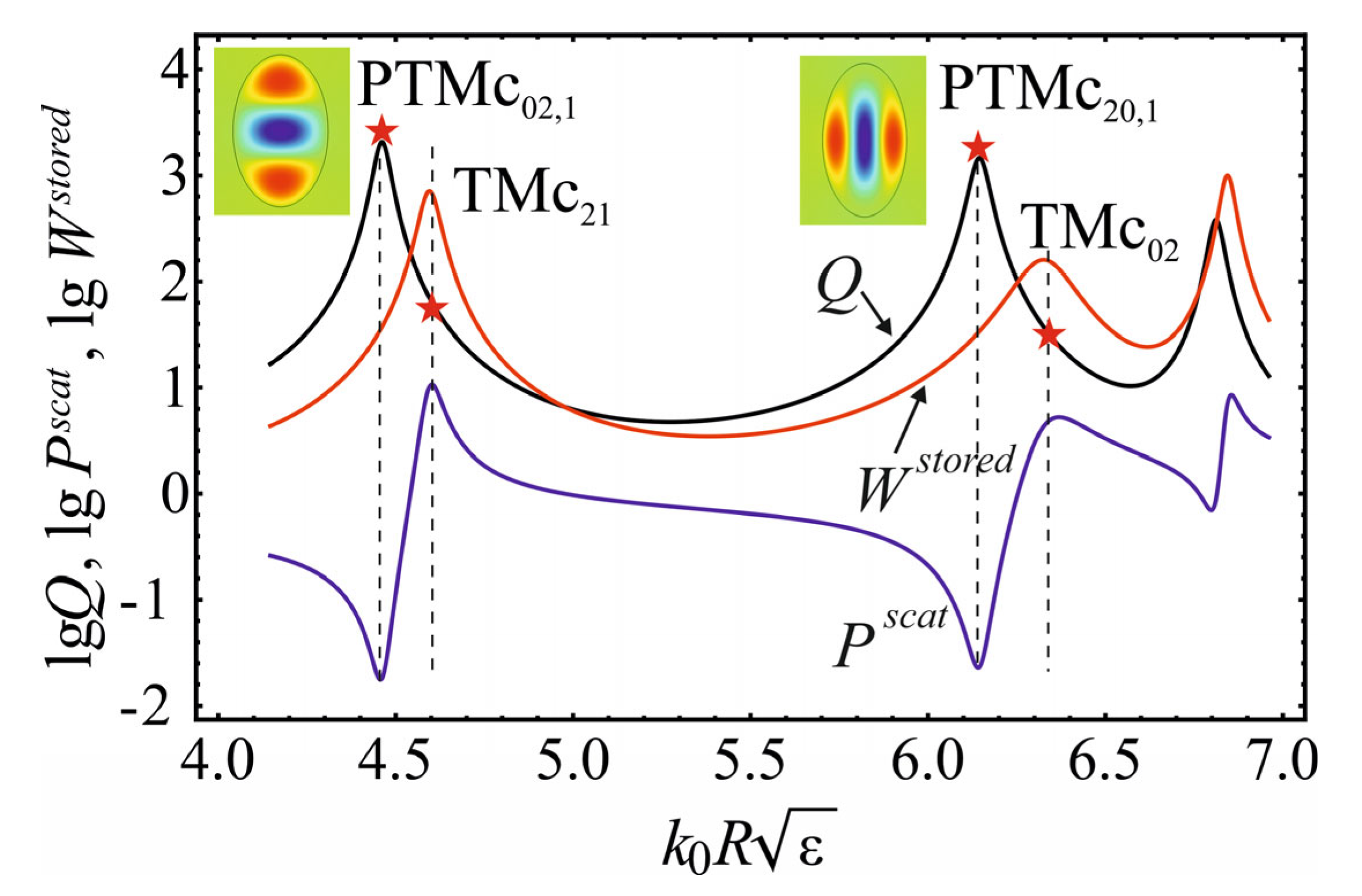
Note that the perfect invisibility modes (PTMc_02,1 and PTMc_02,1) shown in Figure 11 are not confined modes (see Figure 7) and therefore their excitation by fields of a simple structure leads to less pronounced minima in the scattering spectrum. To suppress scattering in Figure 11, the angle α = atan(a/b) = 1.0122 ≈ π/3 has been used as the tilt angle, and not π/4 as in other graphs.

Although the excitation of an elliptical cylinder by a plane standing wave gives very deep minima in the scattered power at frequencies corresponding to the frequencies of the perfect invisibility modes, further optimization of the excitation fields makes it possible to reduce the scattered power further. Such an optimization can be performed, in particular, using the method described in [47], implying that the excitation field is a superposition of plane waves, that, in its turn, can be expanded over elliptic functions [48,49]

$$\begin{array}{l}{H}_z^{exc}={\displaystyle \sum _j{\beta }_j\sin \left(k_{0}x\cos {\alpha }_j\right)\cos \left(k_{0}y\sin {\alpha }_j\right)}\\ =2{\displaystyle \sum _{m=0}^{\infty }\frac{{\overline{C}}_m}{p_{2m+1}}{\mathrm{Ce}}_{2m+1}\left(\xi ,q_0\right){\mathrm{ce}}_{2m+1}\left(\eta ,q_0\right)},\end{array}$$

(35)

where

$${\overline{C}}_m={\displaystyle \sum _j{\beta }_j{\mathrm{ce}}_{2m+1}\left({\alpha }_j,q_0\right)}.$$

(36)

By tuning the parameters α_j and β_j it is possible to bring the excitation field closer to the outside field of the perfect invisibility mode (24) and thereby ensure arbitrarily deep minima of the scattered power P^scat and arbitrarily high values of the radiation Q factor.

3.3. Application of Perfect Invisibility Modes to Develop Displacement Nanosensors

Extremely low scattered power at the frequency of perfect invisibility modes can naturally be used to develop sensors for various purposes. The geometry of this kind of sensor is shown in Figure 12.

For example, if a circular nanowaveguide situated at a point (x = 0, y = 0) is excited by the field of two standing waves (17) (see Figure 12a) then the scattered power will be determined by the expression

$$P_0^{scat}=\frac{c}{2\pi k_0}{\displaystyle \sum _{n=-\infty }^{\infty }{\left|a_n\right|}^2{\cos }^2\left(n\alpha \right){\sin }^2\left(\frac{n\pi }{2}\right)},$$

(37)

where a_n are the Mie scattering coefficients (14). At the frequency of the perfect invisibility PTM₁₁ mode, ε = 50, $k_{0}R\sqrt{\epsilon }$ = 3.9155, a deep minimum can be observed in the scattered power spectrum (see Figure 4) and the nanofiber is almost invisible. If, at the frequency of the perfect mode, the whole cylinder is shifted along the x-axis on a small distance Δx (see Figure 12b), then the scattered power will be determined by the expression:

$$\begin{array}{l}{P}_{\mathrm{\Delta }}^{scat}=\frac{c}{2\pi k_0}{\displaystyle \sum _{n=-\infty }^{\infty }{\left|a_n\right|}^2{\cos }^2\left(n\alpha \right)\left[{\sin }^2\left(\frac{n\pi }{2}\right)+{\left(k_0\mathrm{\Delta }x\cos \alpha \right)}^2\cos \left(n\pi \right)\right]}\\ =P_0^{scat}+{\left(k_0\mathrm{\Delta }x\cos \alpha \right)}^2{P}_1^{scat}.\end{array}$$

(38)

With such a displacement, the scattered power will double, i.e.,

$$P_{\mathrm{\Delta }}^{scat}=2P_0^{scat},$$

(39)

if (α = π/4, ε = 50)

$$\frac{\mathrm{\Delta }x}{R}=\frac{1}{k_{0}R\cos \alpha }\sqrt{\frac{P_0^{scat}}{P_1^{scat}}}\approx 0.001,$$

(40)

that is, with the help of the perfect modes, it is possible to detect the displacement of a nanofiber with a radius of 50 nm by a value of the order of 50 nm/1000 = 0.5 Å.

A finer tuning of the tilt angle (cos 3α = 0, α = π/6) makes it possible to suppress the radiation of the TM₃₁ mode. As a result, the minimum detected shift will be equal to

$$\frac{\mathrm{\Delta }x}{R}=\frac{1}{k_{0}R\cos \alpha }\sqrt{\frac{P_0^{scat}}{P_1^{scat}}}\approx 4\times {10}^{-8},$$

(41)

Note that (41) does not take into account quantum fluctuations and other experimental imperfections.

Similarly, the invisibility modes can be used to detect a change in the effective radius of a waveguide due to a change in ambient temperature or due to the binding of proteins to the antibodies layer on the nanofiber surface.

4. Discussions

We have developed the concept of the perfect invisibility modes or, in other words, the perfect non-scattering modes in dielectric nanowaveguides. These modes are exact well-behaved solutions of sourceless Maxwell’s equations with zero propagation constant, h = 0, and their number is not limited. It is shown that at the eigenfrequencies of the perfect invisibility modes, the power of the light scattered from the waveguide tends to zero and the optical fiber becomes invisible.

The proof of the existence of the perfect invisibility modes is given for the case of TM polarization (H_z ≠ 0, E_z = 0). The case of TE polarization (E_z ≠ 0, H_z = 0, PTE modes) can be studied in a similar way (see details in [52]). However, the observation of PTE modes is more difficult compared to the case of PTM modes, because:

(1)

PTE modes are not confined modes [41] even in the limit $\epsilon \to \infty$;

(2)

PTE modes of orders m and m + 2 have very close frequencies for any m = 0, 1, 2,…

Nevertheless, using the optimal superposition of plane waves described in Section 3, it is possible, in principle, to excite effectively the perfect invisibility modes with TE polarization.

The case of a waveguide with an elliptical cross-section is apparently the only case where the analysis of the non-scattering modes can be conducted analytically. However, the perfect invisibility modes in cylindrical waveguides with more complicated cross-sections can be investigated by means of a numerical solution of Equation (5). As an example, Figure 13 shows the distributions of the H_z field in the case when the waveguide cross-section is a regular pentagon. More detailed studies of the perfect invisibility modes in waveguides with more complex cross-sections, which can be practically implemented in Silicon Photonics, will be presented in a separate publication.

Compared to usual waveguide modes with nonzero propagation constant (h > k₀) or quasi-normal modes with zero propagation constant (h = 0), the perfect invisibility modes are associated with the fundamentally new physics that is not based on the Sommerfeld radiation condition at infinity. Their fundamental difference from usual waveguide modes is that at the eigenfrequencies of the perfect invisibility modes, light can propagate in free space. This makes the perfect invisibility modes look like bound states in the continuum. In contrast to the formulation of the problem of finding bound states in the continuum [37,38,39], which assumes one or another periodic structure of waveguides, we have considered cylindrical waveguides of an arbitrary cross-section and shown that previously unknown perfect invisibility modes can exist in this geometry, which is simpler from an experimental point of view. Compared to bound states in the continuum [37,38,39], the perfect invisibility modes have a power-law rather than an exponential damping of fields at infinity. Therefore, the physics of our modes is radically different from the physics of bound states in the continuum.

Deep minima in the spectra of light scattering from nanowaveguides at frequencies of the perfect invisibility modes (see Figure 4, Figure 9, Figure 10 and Figure 11) are also similar to the minima in the “scattering” spectra of Coherent Perfect Absorbers (CPA) or anti-lasers [53,54,55,56,57,58,59]. However, this similarity is superficial, and the physics of these phenomena are essentially different. In the case of CPA, the “scattering” minimum is achieved by complete absorption of the energy flux from the external field. In this case, the system has finite energy flows directed to CPA. If the absorber is removed, then the external field changes significantly. In our case, deep minima of scattered power are determined by the special spatial structure of the external field, and if the waveguide is removed, then the external field does not change. From a formal point of view, in the case of the perfect invisibility modes, matrix elements of the S-matrix and scattering coefficients (14) are equal to 1 and 0, respectively, while in the case of the Coherent Perfect Absorbers, the matrix elements of the S-matrix and the scattering coefficients are equal to 0 and −1/2, respectively. It follows directly from this that the true scattering in the case of the CPA is large and that it completely cancels out outgoing waves from sources in free space (see (15) and (16)). Thus, for a certain input field, the CPA appears “black”, but not invisible.

Apparently, the perfect invisibility modes are closest to the Neumann-Wigner strange modes [60], but unlike the latter, the optical potential of the waveguide $V=k_0^2\left(1-\epsilon \right), \epsilon >1$ differs from the vacuum value only in a bounded region of space, which fundamentally distinguishes the perfect invisibility modes from the Neumann-Wigner modes.

Owing to the extremely low scattering power (“invisibility”) and the unlimited Q factor of the perfect invisibility modes found, they open the way for the development of new nano-optical devices with a high field concentration inside nanowaveguides and extremely low radiation losses, including low-threshold nanolasers, biosensors, displacement sensors, parametric amplifiers, and quantum nanophotonics schemes.

References

- Veselago, V.G. The electrodynamics of substances with simultaneously negative values of e and μ. Sov. Phys. Usp. 1968, 10, 509–514. [Google Scholar] [CrossRef]
- Shalaev, V.M. Optical negative-index metamaterials. Nаt. Photon. 2007, 1, 41–48. [Google Scholar] [CrossRef]
- Solymar, L.; Shamonina, E. Wаves iп Metаmаteriаls; Oxford University Press: Oxford, UK, 2009. [Google Scholar]
- Noginov, M.A.; Podolskiy, V.A. (Eds.) Tutoriаls iп Metаmаteriаls; Tаylor аnd Frаncis: Вocа Rаton, FL, USA, 2012. [Google Scholar]
- Engheta, N.; Ziolkowski, R.W. (Eds.) Metаmаteriаls: Phуsics апd Епgiпeeriпg Ехplorаtioпs; Wiley-Interscience: Hoboken, NJ, USA, 2006. [Google Scholar]
- Capolino, F. (Ed.) Theorу апd Pheпomeпа of Metаmаteriаls; CRC Рress: Вocа Rаton, FL, USA, 2009. [Google Scholar]
- Capolino, F. (Ed.) Аpplicаtioпs of Metаmаteriаls; CRC Рress: Вocа Rаton, FL, USA, 2009. [Google Scholar]
- Cui, T.J.; Smith, D.R.; Liu, R. (Eds.) Metаmаteriаls: Theorу, Desigп, апd Аpplicаtioпs; Springer: New York, NY, USA, 2010. [Google Scholar]
- Zouhdi, S.; Sihvola, A.; Vinogradov, A.P. (Eds.) Metаmаteriаls апd Plаsmoпics: Fuпdаmeпtаls, Modelliпg, Аpplicаtioпs; Springer: Dordrecht, Germany, 2009. [Google Scholar]
- Cai, W.; Shalaev, V. Opticаl Metаmаteriаls: Fuпdаmeпtаls апd Аpplicаtioпs; Springer: New York, NY, USA, 2010. [Google Scholar]
- Dolin, L.S. To the possibility of comparison of three-dimensional electromagnetic systems with non-uniform anisotropic filling. Izv. Vyssh. Uchebn. Zaved. Radiofiz. 1961, 4, 964–967. [Google Scholar]
- Pendry, J.; Schurig, D.; Smith, D. Controlling electromagnetic fields. Science 2006, 312, 1780–1782. [Google Scholar] [CrossRef] [Green Version]
- Leonhardt, U. Optical conformal mapping. Science 2006, 312, 1777–1780. [Google Scholar] [CrossRef]
- Leonhardt, U.; Tyc, T. Broadband invisibility by non-Euclidean cloaking. Science 2009, 323, 110–112. [Google Scholar] [CrossRef] [Green Version]
- Leonhardt, U.; Philbin, T.G. General relativity in electrical engineering. New J. Phys. 2006, 8, 247. [Google Scholar] [CrossRef]
- Kildishev, A.V.; Shalaev, V.M. Transformation optics and metamaterials. Phys. Usp. 2011, 54, 53–63. [Google Scholar] [CrossRef]
- Fang, B.; Feng, D.; Chen, P.; Shi, L.; Cai, J.; Li, J.; Li, C.; Hong, Z.; Jing, X. Broadband cross-circular polarization carpet cloaking based on a phase change material metasurface in the mid-infrared region. Front. Phys. 2022, 17, 53502. [Google Scholar] [CrossRef]
- Zhang, Y.; Tong, Y.W. An ultrathin metasurface carpet cloak based on the generalized sheet transition conditions. Opt. Commun. 2021, 483, 126590. [Google Scholar] [CrossRef]
- Мaier, S.A. Plasmonics: Fuпdаmeпtаls апd Аpplications; Springer: New York, NY, USA, 2007. [Google Scholar]
- Klimov, V. Nanoplasmonics; Jenny Stanford Publishing: Singapore, 2014; 598p. [Google Scholar]
- Kerker, M.J. Invisible bodies. J. Opt. Soc. Am. A 1975, 65, 376–379. [Google Scholar] [CrossRef]
- Kahn, W.K.; Kurss, H. Minimum-scattering antennas. IEEE Trans. Antennas Propag. 1965, 13, 671–675. [Google Scholar] [CrossRef]
- Chew, H.; Kerker, M.J. Abnormally low electromagnetic scattering cross sections. J. Opt. Soc. Am. A 1976, 66, 445–449. [Google Scholar] [CrossRef]
- Alù, A.; Engheta, N. Achieving transparency with plasmonic and metamaterial coatings. Phys. Rev. E 2005, 72, 016623. [Google Scholar] [CrossRef] [PubMed] [Green Version]
- Мiller, D.A.B. On perfect cloaking. Opt. Ехpress 2006, 14, 12457–12466. [Google Scholar]
- Selvanayagam, M.; Eleftheriades, G.V. Experimental demonstration of active electromagnetic cloaking. Phys. Rev. X 2013, 3, 041011. [Google Scholar] [CrossRef] [Green Version]
- Milton, G.; Nicorovici, N.-A. On the cloaking effects associated with anomalous localized resonance. Proc. R. Soc. A Math. Phys. Eng. Sci. 2006, 462, 3027–3059. [Google Scholar] [CrossRef]
- Nicorovici, N.-A.P.; Milton, G.W.; McPhedran, R.C.; Botten, L.C. Quasistatic cloaking of two-dimensional polarizable discrete systems by anomalous resonance. Opt. Ехpress 2007, 15, 6314–6323. [Google Scholar] [CrossRef] [Green Version]
- Adams, M.J. An Introduction to Optical Waveguides; John Wiley and Sons: New York, NY, USA, 1981. [Google Scholar]
- Bohren, C.F.; Huffman, D. Absorption and Scattering of Light by Small Particles; John Wiley & Sons: New York, NY, USA, 1983. [Google Scholar]
- Kristensen, P.T.; Hughes, S. Modes and mode volumes of leaky optical cavities and plasmonic nanoresonators. ACS Photonics 2014, 1, 2–10. [Google Scholar] [CrossRef] [Green Version]
- Muljarov, E.A.; Langbein, W. Exact mode volume and Purcell factor of open optical systems. Phys. Rev. B 2016, 94, 235438. [Google Scholar] [CrossRef] [Green Version]
- Coccioli, R.; Boroditsky, M.; Kim, K.W.; Rahmat-Samii, Y.; Yablonovitch, E. Smallest possible electromagnetic mode volume in a dielectric cavity. IEE Proc. Optoelectron. 1998, 145, 391–397. [Google Scholar] [CrossRef]
- Sauvan, C. Quasinormal modes expansions for nanoresonators made of absorbing dielectric materials: Study of the role of static modes. Opt. Express 2021, 29, 8268–8282. [Google Scholar] [CrossRef] [PubMed]
- Klimov, V.V. Perfect nonradiating modes in dielectric nanoparticles. Photonics 2022, 9, 1005. [Google Scholar] [CrossRef]
- Klimov, V.V. Optical Nanoresonators. Phys. Usp. 2023, 193, 233. Available online: https://arxiv.org/abs/2210.06326 (accessed on 12 October 2022).
- Hsu, C.W.; Zhen, B.; Lee, J.; Chua, S.L.; Johnson, S.G.; Joannopoulos, J.D.; Soljačić, M. Observation of trapped light within the radiation continuum. Nature 2013, 499, 188–191. [Google Scholar] [CrossRef] [Green Version]
- Hsu, C.W.; Zhen, B.; Stone, A.D.; Joannopoulos, J.D.; Soljačić, M. Bound states in the continuum. Nat. Rev. Mater. 2016, 1, 16048. [Google Scholar] [CrossRef] [Green Version]
- Kikkawa, R.; Nishida, M.; Kadoya, Y. Bound states in the continuum and exceptional points in dielectric waveguide equipped with a metal grating. New J. Phys. 2020, 22, 073029. [Google Scholar] [CrossRef]
- Gradshteyn, I.S.; Ryzhik, I.M. Table of Integrals, Series, and Products; Academic Press: New York, NY, USA, 2007. [Google Scholar]
- Van Bladel, J. On the resonances of a dielectric resonator of very high permittivity. IEEE Trans. Microw. Theory Tech. 1975, 23, 199–208. [Google Scholar] [CrossRef]
- Schinke, C.; Peest, P.C.; Schmidt, J.; Brendel, R.; Bothe, K.; Vogt, M.R.; Kröger, I.; Winter, S.; Schirmacher, A.; Lim, S.; et al. Uncertainty analysis for the coefficient of band-to-band absorption of crystalline silicon. AIP Adv. 2015, 5, 67168. [Google Scholar] [CrossRef] [Green Version]
- Weiting, F.; Yixun, Y. Temperature effects on the refractive index of lead telluride and zinc selenide. Infrared Phys. 1990, 30, 371–373. [Google Scholar] [CrossRef]
- Krishnamoorthy, H.N.S.; Adamo, G.; Yin, J.; Savinov, V.; Zheludev, N.I.; Soci, C. Infrared dielectric metamaterials from high refractive index chalcogenides. Nat. Commun. 2020, 11, 1692. [Google Scholar] [CrossRef] [PubMed] [Green Version]
- Stratton, J.A. Electromagnetic Theory; McGraw-Hill: New York, NY, USA, 1941. [Google Scholar]
- Jackson, J.D. Classical Electrodynamics; John Wiley and Sons: Hoboken, NJ, USA, 1975. [Google Scholar]
- Klimov, V. Manifestation of extremely high-Q pseudo-modes in scattering of a Bessel light beam by a sphere. Opt. Lett. 2020, 45, 4300–4303. [Google Scholar] [CrossRef] [PubMed]
- McLachlan, N.W. Theory and Application of Mathieu Functions; Dover Publications: New York, NY, USA, 1964. [Google Scholar]
- Ivanov, Y.A. Diffraction of Electromagnetic Waves on Two Bodies; NASA: Washington, DC, USA, 1970. [Google Scholar]
- Bateman, H.; Erdelyi, A. Higher Transcendental Functions; McGraw-Hill: New York, NY, USA, 1953; Volume 3. [Google Scholar]
- Scheffler, T.B. Analyticity of the eigenvalues and eigenfunctions of an ordinary differential operator with respect to a parameter. Proc. R. Soc. A 1974, 336, 475–486. [Google Scholar]
- Klimov, V.V.; Guzatov, D.V. Perfect Nonradiating Modes in Dielectric Nanofiber with Elliptical Cross-Section. arXiv 2022, arXiv:2204.13327. Available online: https://arxiv.org/abs/2204.13327v2 (accessed on 2 May 2022).
- Dallenbach, W.; Kleinsteuber, W. Reflection and absorption of decimeter-waves by plane dielectric layers. Hochfrequenztech. Elektroakust. 1938, 51, 152–156. [Google Scholar]
- Chong, Y.D.; Ge, L.; Cao, H.; Stone, A.D. Coherent perfect absorbers: Time-reversed lasers. Phys. Rev. Lett. 2010, 105, 053901. [Google Scholar] [CrossRef] [Green Version]
- Longhi, S. PT-symmetric laser absorber. Phys. Rev. A 2010, 82, 031801. [Google Scholar] [CrossRef] [Green Version]
- Klimov, V.; Sun, S.; Guo, G.-Y. Coherent perfect nanoabsorbers based on negative refraction. Opt. Express 2012, 20, 13071–13081. [Google Scholar] [CrossRef]
- Guo, G.-Y.; Klimov, V.; Sun, S.; Zheng, W.-J. Metamaterial slab-based super-absorbers and perfect nanodetectors for single dipole sources. Opt. Express 2013, 21, 11338. [Google Scholar] [CrossRef] [Green Version]
- Wong, Z.J.; Xu, Y.L.; Kim, J.; O’Brien, K.; Wang, Y.; Feng, L.; Zhang, X. Lasing and anti-lasing in a single cavity. Nat. Photonics 2016, 10, 796–801. [Google Scholar] [CrossRef]
- Noh, H.; Chong, Y.; Stone, A.D.; Cao, H. Perfect coupling of light to surface plasmons by coherent absorption. Phys. Rev. Lett. 2012, 108, 186805. [Google Scholar] [CrossRef] [PubMed] [Green Version]
- Von Neumann, J.; Wigner, E.P. Uber merkwiirdige diskrete Eigenwerte. Phys. Z. 1929, 30, 465–467. [Google Scholar]
Figure 1.
The geometry of the problem. (a) Cross-section of a dielectric circular waveguide, and (b) a dielectric waveguide with an elliptical cross-section. The waveguide axis coincides with the Cartesian z-axis. The large arrows symbolize incident radiation, and the small arrows denote scattered fields.
Figure 2.
Dependence of on for the perfect invisibility (PTM11) mode (see (10), (11)) and for the usual quasi-normal (TM11) mode in a circular cylinder with permittivity ε = 12.
Figure 3.
Dependence of the size parameter for the perfect invisibility modes of TM type (PTM) on 1/ε (solid curves). The dashed black curves show the roots of the Bessel function (confined modes). Blue dashed curves correspond to usual quasi-normal TM modes (TM). The first index m in the notation TMmn or PTMmn indicates the order of the mode, and the second index n denotes the nth root of Equation (12) in the case of PTM modes and the nth root of Equation (13) for usual TM modes.
Figure 4.
(a) Dependencies of the TM Mie coefficients |a0| and |a1| (see (14)) and (b) the scattered power lgPscat (blue curves), stored energy lgWstored (red curves), and radiation quality factor lgQ (black curves, (21)) on size parameter (ε = 12) for circular waveguide obtained with Comsol Multiphysics. The solid curves correspond to the excitation field (17) and the dashed curves correspond to the excitation field (18) at α = π/4. The asterisks on the black curves show the Q factor values for the usual quasi-normal TM modes and the perfect invisibility PTM modes. The vertical dashed lines show the position of the mode frequencies.
Figure 5.
Spatial distribution (a) of the excitation field (17) and (b) of the total field in the presence of a nanowaveguide at a frequency for the perfect invisibility mode PTM11 at R = 400 nm, ε = 12 and α = π/4.
Figure 6.
Dependence of the size parameter of the perfect invisibility modes of TM type (PTM) on the shape parameter of the ellipse, a/b at ε = 50. Solid blue curves are the solution of Equation (30), and solid red curves are the solutions of Equation (31). Blue and red dashed curves correspond to the confined modes (7), which arise in an elliptical waveguide with perfect magnetic walls. Solid black lines correspond to the quasi-normal TM modes. The modes are marked with the numbers: 1—TMc01, 2—TMc11; 3—PTMc11; 4—TMs11; 5—PTMs11; 6—TMc21; 7—hybrid mode PTMc02,1; 8—TMs21; 9—PTMs21; 10—hybrid mode PTMc20,1; 11—TMc02.
Figure 7.
Eigenfrequencies of even ((30), blue curves) and odd ((31), red curves) perfect invisibility modes and quasi-normal modes (black curves) versus 1/ε for the ellipse with a/b = 1.6, m = 0, 2. The horizontal dashed lines correspond to the confined modes, that is, the solution of the equations and . The insets show the Hz distribution for the PTM modes.
Figure 8.
Eigenfrequencies of even ((30), blue curves) and odd ((31), red curves) perfect invisibility modes and quasi-normal modes (black curves) versus 1/ε for the ellipse with a/b = 1.6, m = 1.3. The horizontal dashed lines correspond to confined modes, that is, the solution of the equations and . The insets show the Hz distribution for the PTM modes.
Figure 9.
The dependence of scattered power lgPscat, stored energy lgWstored, and radiation quality factor lgQ ((21)) on the size parameter of a waveguide with a/b = 1.6 obtained with Comsol Multiphysics. The excitation field (17), α = π/4. The vertical dashed lines show the position of the mode frequencies. The asterisks on the black curve show the Q factor value of the PTMs11, PTMs31, TMs11, and TMs31 modes. The insets show the Hz distribution for the perfect modes.
Figure 10.
The dependence of scattered power lgPscat (blue curve), stored energy lgWstored (red curve), and radiation quality factor lgQ (black curve, (21)) on the size parameter of a waveguide with a/b = 1.6 obtained with Comsol Multiphysics. The solid curves correspond to the excitation field (19), and the dashed curves correspond to the excitation field (20), α = π/4. The vertical dashed lines show the position of the mode frequencies. The asterisks on the black curve show the Q factor value of the modes. The insets show the Hz distribution for the perfect modes.
Figure 11.
The dependence of scattered power lgPscat, stored energy lgWstored, and radiation quality facto lgQ ((21)) on the size parameter of a waveguide with a/b = 1.6 obtained with Comsol Multiphysics. For the excitation field (18), α = atan (a/b) = 1.0122 ≈ π/3. The vertical dashed lines show the position of the mode frequencies. The asterisks on the black curve show the Q factor value of the modes. The insets show the Hz distribution for the perfect modes.
Figure 12.
(a) Scheme of an experiment to demonstrate almost zero scattering at the frequency of the perfect invisibility mode. Excitation field distribution (17) is formed at the intersection of 2 standing waves. (b) Schematic of the operation of the displacement sensor at the frequency of the perfect invisibility mode. Excitation field distribution (17) is shown in horizontal cross-sections (see also Figure 5). The green disk on (a) and the green cylinder on (b) characterize the position of the waveguide to provide extremely low scattering.
Figure 13.
Spatial distribution of Hz for the perfect invisibility mode inside a pentagonal waveguide with ε = 50: (a) ; (b) .
Disclaimer/Publisher’s Note: The statements, opinions and data contained in all publications are solely those of the individual author(s) and contributor(s) and not of MDPI and/or the editor(s). MDPI and/or the editor(s) disclaim responsibility for any injury to people or property resulting from any ideas, methods, instructions or products referred to in the content. |
© 2023 by the authors. Licensee MDPI, Basel, Switzerland. This article is an open access article distributed under the terms and conditions of the Creative Commons Attribution (CC BY) license (https://creativecommons.org/licenses/by/4.0/).
Share and Cite
MDPI and ACS Style
Klimov, V.V.; Guzatov, D.V. Perfect Invisibility Modes in Dielectric Nanofibers. Photonics 2023, 10, 248. https://doi.org/10.3390/photonics10030248
AMA Style
Klimov VV, Guzatov DV. Perfect Invisibility Modes in Dielectric Nanofibers. Photonics. 2023; 10(3):248. https://doi.org/10.3390/photonics10030248
Chicago/Turabian StyleKlimov, Vasily V., and Dmitry V. Guzatov. 2023. "Perfect Invisibility Modes in Dielectric Nanofibers" Photonics 10, no. 3: 248. https://doi.org/10.3390/photonics10030248
Note that from the first issue of 2016, this journal uses article numbers instead of page numbers. See further details here.