1. Introduction
Cavity optomechanics describes the coupling behavior between the optical resonators and the mechanical resonators within an optical cavity [
1]. The optically induced mechanical damping rate can be positive (leads to mechanical cooling) or negative (leads to mechanical amplification), depending on whether the pump laser is red-detuned or blue-detuned to the optical resonance [
2,
3]. Once the overall damping rate of the mechanical mode is negative in the blue-detuned regime, self-sustained oscillation of the mechanical mode occurs. This is also known as mechanical lasing or phonon lasing [
4]. Single-mechanical-mode lasing has been extensively explored in whispering-gallery-mode (WGM) and Fabry–Perot (F–P) microcavities [
5,
6,
7,
8,
9,
10,
11,
12]. Optomechanical coupling efficiency can be high because the optical resonator has a high quality factor (Q) and a small mode volume [
13]. On the other hand, multimode phonon lasing can serve as a new research method for the exploration of physical phenomena such as self-organized synchronization [
14,
15,
16,
17] and acoustic frequency combs [
18]. However, there are much fewer references on multimode phonon lasing. In fact, optical resonance in the cavity can couple with multiple mechanical modes simultaneously. However, only one mechanical mode can reach the threshold condition of stimulated oscillation because of the mechanical mode competition [
18,
19,
20]. Additional controls are necessary to achieve simultaneous multiple mechanical mode lasing in an optomechanical system, which includes adding multiple mechanical vibration structures into the system [
15,
16], using multiple beat frequencies generated between multiple incident lasers to resonate with multiple mechanical modes [
21], or using mode-locking techniques [
18].
In the field of optical lasers, multiple longitudinal mode lasing techniques have been investigated. In 1964, Lamb found that, theoretically, when two lasing modes are in the strong coupling regime, mode competition leads to single-mode lasing. On the other hand, when two lasing modes are in the weak coupling regime, multimode lasing is allowed [
22]. Mode competition effects have also been observed in Raman lasers, and single-mode switching or dual-mode Raman lasing can be achieved with the suitable system parameters [
23,
24]. Therefore, studying the analogous issue in an optomechanical system and investigating the relation of multiple mechanical modes lasing with the coupling strength would be interesting and important.
In this paper, we first derived the expressions of mode-coupling coefficients whereby an optical resonant mode is coupled to two mechanical modes. The simulation results revealed that dual-mode lasing exists when two mechanical modes couple weakly. Experimentally, we observed dual-mechanical-mode lasing in a microbubble optical resonator. As theory predicts, the intensities of the two lasing modes modulate when the optical pump intensity changes. We also confirmed from the experimental results that the system is truly in a weak coupling condition. This work, while further demonstrating the analogy of optomechanical phonon lasers to optical lasers, also helps to simplify the design of the optomechanical systems that facilitate the simultaneous stable lasing of multiple mechanical modes and provides guidance for future research into optomechanical acoustic frequency combs.
2. Two Mechanical Modes Coupling Theory in Optomechanical System
If we consider an optomechanical system in which a high-Q optical resonant mode couples with two mechanical modes in whispering-gallery-mode microcavity (in our case it is a microbubble resonator, MBR [
25,
26]), the oscillation modulation can be understood as follows. The change in the amplitude of one mechanical mode will lead to a change in the optical resonance frequency. Then, the amplitude of the intracavity optical field changes, which in turn will change the optically induced damping rate of both the mechanical modes.
To theoretically manage the coupling of the mechanical modes in an MBR, we follow the framework in which one optical mode couples with multiple mechanical modes in the (WGM/F–P) microcavity proposed in Ref. [
13] and with the solution process of the F-P cavity system shown in Ref. [
19].
The circulating optical field in an MBR with radius
R is denoted by
, it exerts circulating radiation pressure
on the cavity boundary, and the equation is as follows [
5,
13]:
In which the optical field loss rate is , where describes the intrinsic cavity loss rate, and describes the loss rate of the optical field when it couples to an MBR optical mode from a tapered fiber. is the pump laser power, and the detuning is the angular frequency difference between the pump laser and the optical resonance (i.e., ). is the time-dependent change in the MBR radius.
When two mechanical modes A and B are coupled to one optical resonant mode simultaneously,
can be expressed as follows [
13]:
where
n = A or B,
is the one-dimensional equivalent amplitude of the three-dimensional mechanical mode distribution,
is a number in the range of 0–1 that determines the relative transduction strength of
in
[
13], and
is the mechanical mode frequency. Thus, Equation (1) can be written as follows:
Meanwhile,
follows the motional equation [
13]:
where
is the effective mass of the mechanical mode,
is the thermal Langevin force, and
is the mechanical damping rate of the mode.
is the optically induced damping rate of the mechanical mode, which is determined by the effective radiation pressure
[
13,
19].
After obtaining
with Equation (3), we can further identify
, and then obtain
as follows [
19]:
where
are the dimensionless parameters used to describe the mechanical mode amplitude
more concisely. Equations (5) and (6) are more or less similar to that in Ref. [
19], which was derived for determining the F–P cavity. However, the expression before the imaginary part is for the whispering-gallery-mode cavity. The two equations clearly show that the damping rate of mode A and B comes from the behavior of both modes, i.e., there is coupling between the two mechanical modes. It should be noted that the coupling between the mechanical modes is not direct but occurs through the optical mode.
To describe the coupling strength between the mechanical modes in the optomechanical system, we follow the procedure of multimode optical lasing, and derive the change of the gain coefficients of the two modes as follows [
22]:
where
describes the intensity of the mechanical mode,
is the self-saturation coefficient, and
and
are cross-saturation coefficients. The cross-saturation coefficients reflect how much one mode is suppressed by the other mode. In optical laser technology, the coupling coefficient
C is used to identify the coupling state of the two modes [
22]:
The larger the value of
C, the stronger the coupling between the two modes will be.
C > 1 is the strong coupling region, where the cross-saturation between the two mechanical modes is stronger than the self-saturation effect, and the competition between two modes is so strong that only one mode involves stable lasing.
C < 1 is the weak coupling region, where the cross-saturation between the two mechanical modes is weaker than the self-saturation, and the two-modes competition allows both modes to establish stable lasing [
22]. According to Equation (4), the gain of the n
th mode can be written as:
, where
is fixed. So, the total derivative of
is:
When the pump power is fixed, Equations (10) and (11) can be simplified as:
By comparing the above equations with Equations (7) and (8), self-saturation coefficients
and
can be derived from
and
, and the cross-saturation coefficients
and
can be derived from
and
. According to Equation (9), the coupling coefficient between the mechanical modes is:
In an MBR optomechanical system where two mechanical modes oscillate simultaneously, when the optically induced gain of both mechanical modes exceeds their intrinsic loss, the subsequent evolution of these modes will depend on the strength of their coupling. In this process, due to the optical mode and mechanical modes having been determined, the parameters , , in Equations (5) and (6) will be fixed. Combining Equations (5), (6) and (14), it can be noted that, for an MBR optomechanical system with dual-mode oscillation, the parameters affecting the C are mainly the optical mode Q value, the pump laser detuning , and . is determined by both the pump laser power and .
Here, we provide the simulation results. Consider an MBR optomechanical system that has a radius of cavity
,
,
,
,
,
, and
, with the radial/axial/angular quantum numbers for the two mechanical modes being 1/2/1 and 1/3/3, respectively. The intrinsic damping rate of the two mechanical modes is taken as
and
, values which are similar to some WGM optomechanical systems observed so far (
[
27];
[
28]). The effective mass of the two mechanical modes is calculated by performing finite element simulation as
, and
. In addition, assume
, and
such that the pump power range where mode intensity modulation occurs is similar to that in the experiment. The ratio of detuning to the optical field loss rate is 0.8 (i.e.,
).
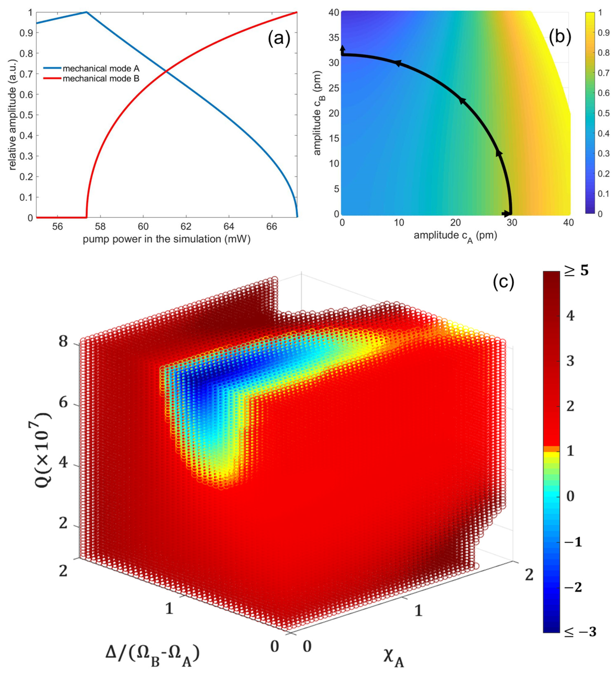
Figure 1a plots the change in mechanical mode intensity as a function of optical power in the cavity, which is calculated by Equations (4)–(6). As
increases from 55.00 mW to 67.18 mW, the intensity of the two mechanical modes will change oppositely in response to the change in pump power. This is because when the intensity of mechanical mode B increases, it depletes more energy from the intracavity optical field, leaving less energy for mechanical mode A and resulting in a decrease in its intensity.
Figure 1b plots the weak coupling region according to Equation (14) and marks the intensity changes of the two mechanical modes in the above simulation results with black curves. As the intensity changes, the coupling coefficient decreases. This is because when the mechanical mode B is also lased, the amplitude of the mechanical mode B changes more significantly within one cycle, causing the corresponding intracavity intensity variation to be more severe. This results in the optically induced damping rate of the mechanical mode B being more affected by its amplitude changes compared to when it is not lased. As a result, the coupling coefficient decreases. Therefore, the highest coupling coefficient is reached at the point when one mode is in lasing and the second mode is at the lasing threshold; when the highest coupling coefficient is still less than 1, it will be able to observe two weakly coupled stimulated oscillating mechanical modes with increased
. To determine the weak coupling region that supports these two modes of stimulated oscillating, the relationship between the highest coupling coefficient value and the parameters must be studied. In this process, the amplitude of the second mechanical mode can be disregarded as it is not yet in lasing.
Figure 1c plots the coupling coefficient as a function of the optical mode Q value, the detuning D, and the dimensionless amplitude
, which are calculated by Equations (5), (6) and (14).
varies from 0 to 2,
Q ranges from
to
, and D is between 0–2 of
. The other parameters are the same as those used in previous calculations. As shown in
Figure 1c,
C is comparatively lower when Δ ≈
. This is due to the high-frequency sidebands generated by the modulation of the pump laser by the oscillation of mechanical mode A, which exerts a relatively stronger gain on mechanical mode B. This ultimately causes the numerator in Equation (14) to decrease or become negative. In addition, when Q is higher,
C is less. This is because the higher the Q factor is, the narrower the optical mode, and the more significant the intracavity intensity variation caused by the cavity boundary oscillation will be, causing
to be more severely affected by the changes brought by
and resulting in an increase in the denominator of Equation (14).
4. Results and Discussion
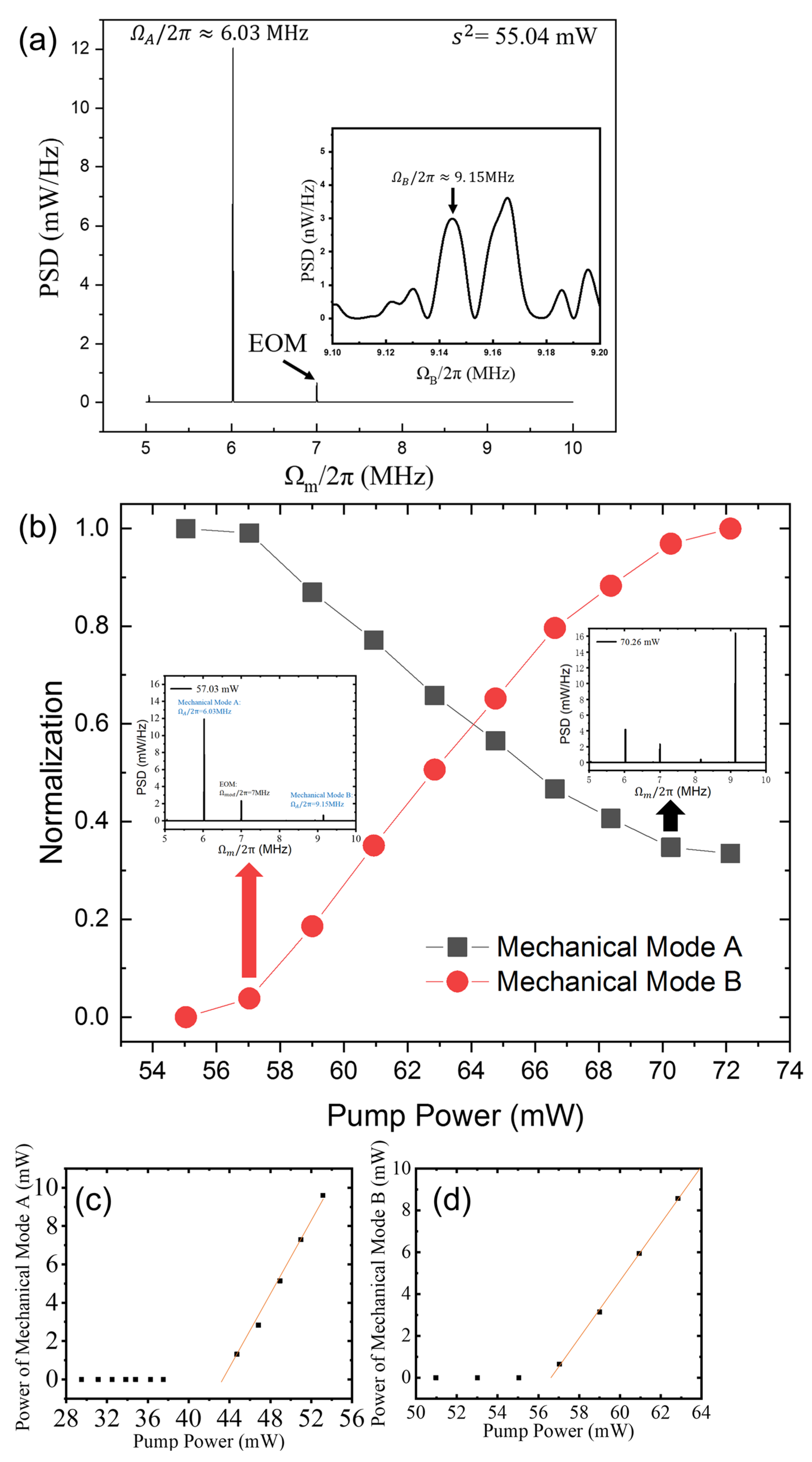
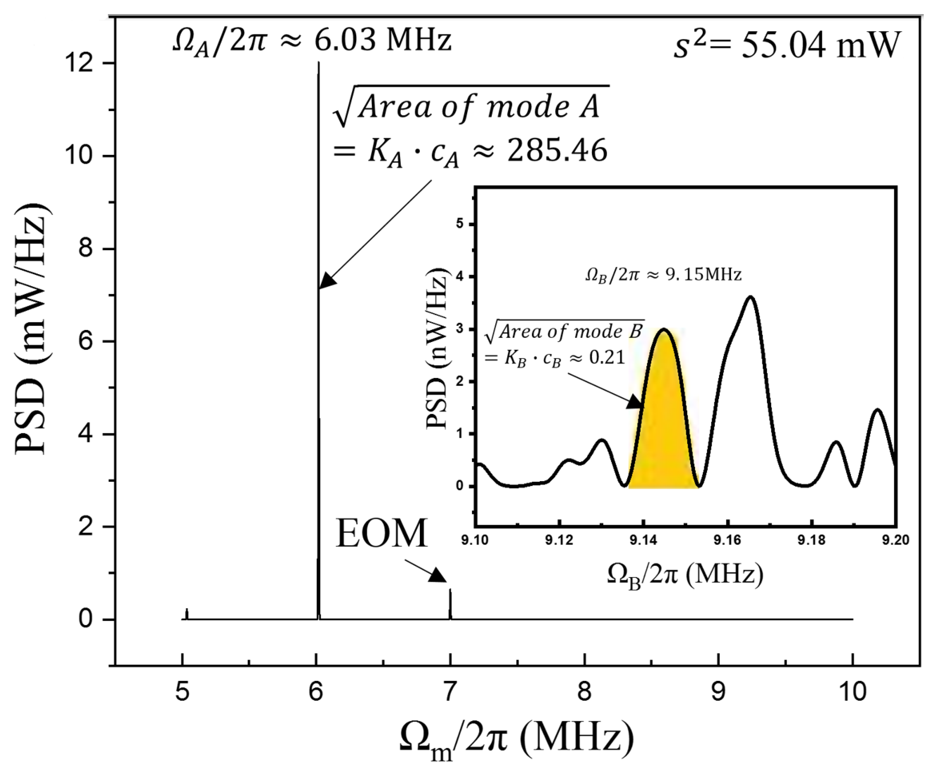
Figure 3a plots a spectrum in a range of 5 to 10 MHz. When the tunable laser wavelength is fixed to an optical mode with a
, the pump laser power is
Mechanical mode A at
and the modulation frequency of the EOM at 7 MHz are observed.
Figure 3b plots the changes in mechanical mode intensity when pump laser power increases from 55.04 mW to 72.13 mW. A second mechanical mode, mode B at
, can be observed clearly at a laser power of 57.03 mW, and its intensity rises continuously. Meanwhile, the intensity of mode A drops to about 30% when the laser pump reaches 72.13 mW.
Figure 3c,d plot the variation of the intensity of mechanical modes A and B at different pump powers, respectively. The stimulated oscillation thresholds of modes A and B are 43.69 mW and 56.57 mW, respectively.
The experimental results show that when the pump power is above 56.57 mW, both mode A and B lase. Their lasing intensities change in opposite ways when pump power increases further. This modulation of the oscillation intensity is analogous to the modulation of laser intensity of two weakly coupled laser modes in a Zeeman laser [
30], in which the intensity of the two laser modes changes oppositely.
As mentioned above, the coupling coefficient
C is the highest when mode A is lasing and mode B is at lasing threshold (
,
). If
C < 1 at this state, the coupling will be weaker when the pump laser power is higher. The detailed coupling coefficient estimation process is provided in the
Appendix A, using Equations (10), (11) and (14) and experimental data.
Finally, the coupling coefficient
C can be obtained as follows:
In this calculation, the power spectral density area measurement for mechanical mode B that does not satisfy the threshold condition is assumed to have a ±15% error (corresponding to an error of −7.8% to +7.2% of ), and a ±0.8% error is assumed regarding the measurement of the pump laser power when mechanical mode B is about to lase (corresponding to an upper limit of power error exactly close to 57.03 mW). As such, we are able to obtain the error range of C in (0.561, 0.997). Therefore, the state of mechanical mode B when it is about to lase (, ) is exactly in the weak coupling region.


