Image Contrast Enhancement by Using LED Annular Oblique Illumination in Bright-Field Microscopy

Abstract

Köhler illumination is the most used method for evenly illuminating a sample in bright-field microscopy. However, Köhler illumination cannot provide optimum contrast and high resolution simultaneously. The image contrast for Köhler illumination can be enhanced at the expense of lateral resolution. In this paper, we discuss the main causes of contrast loss with Köhler illumination by simulating unsymmetrical interference, incoherent superposition, and modulation transfer function. We present a method to increase the image contrast by combining the annular oblique illumination with normalization and blind deconvolution. With the progress of optoelectronic devices, the greater advantages of annular oblique illumination will become apparent. The experimental results achieved by using LED annular oblique illumination prove the feasibility of the proposed method.

1. Introduction

The bright-field microscope is a simple and practical tool [1,2]. Although numerous advanced microscopes have been developed, the bright-field microscope will still be an irreplaceable tool in many fields, especially in pathologic diagnosis. Therefore, it is still one of the goals of microscopists to improve the performance of the bright-field microscope.

Resolution and contrast (visibility) are generally considered as the two main factors affecting image quality in bright-field microscopy. How to obtain a bright-field image with optimum contrast and high resolution has always been a challenge. It is well known that Köhler illumination is the predominant technique in a modern bright-field microscope due to its evenness and high brightness. However, it is impossible to optimize the contrast while maintaining the highest lateral resolution [2,3]. An experienced observer usually increases the contrast by reducing the illumination numerical aperture ($NA$) at the expense of lateral resolution [1,2]. This is why microscope tutorials generally provide a guideline that suggests stopping down the condenser aperture to about 70% of its maximum diameter in order to optimize the contrast [2]. It is necessary to discuss the causes of contrast loss.

In this paper, we discuss the main causes of contrast loss for Köhler illumination: unsymmetrical interference, and incoherent superposition. In addition, we use the modulation transfer function (MTF) to explain that annular oblique illumination can be used to increase contrast for imaging [4,5,6,7,8,9,10]. In the past, annular oblique illumination was produced by a thin ring diaphragm. Due to its unevenness and low brightness, annular oblique illumination was not appropriate for photographic film. As a result, annular oblique illumination lost out to Köhler illumination at that time. However, with the progress of optoelectronic devices, an annular LED array can be employed to create uniform and high-brightness annular oblique illumination [5,6,7,8], and many image processing algorithms can be used to further improve the image quality. In this paper, we present a method to increase the image contrast by combining annular oblique illumination with normalization, and blind deconvolution [11,12]. The experimental and simulated results have demonstrated the feasibility of the proposed method.

2. Principle

2.1. Köhler Illumination

The optical path of Köhler illumination is illustrated in Figure 1. For simplicity, it is composed of two lenses. The image of the light filament in the aperture diaphragm is called the “effective light source”. It is assumed that all points in the effective light source are completely incoherent. The condenser Point A creates the axial illumination, while Point B creates the largest-angle oblique illumination. The sample is illuminated by a solid-cone beam. Thus, the Köhler-illuminated image can be considered as an incoherent superposition of coherent images.

According to Abbe’s theory, a coherent image reproducing the characteristic features of a sample is formed by interfering diffraction orders passed by the objective lens. For simplicity, we assume that only three diffraction orders can pass the objective pupil. The diffraction orders corresponding to the axial illumination and the largest-angle oblique illumination are shown in Figure 2. $f_1$ is the focal length of the objective and $f_2$ is the focal length of the tube lens. As illustrated in Figure 2, for axial illumination, the diffraction order in the pupil plane is symmetrical: A₀, A₋₁ and A₊₁. However, for oblique illumination, the diffraction order is three unsymmetrical diffraction orders: B₀, B₊₁ and B₊₂.

In an ideal system, the image (interference fringe) $I\left(x,y\right)$ formed by diffraction orders can be described by:

$$I\left(x,y\right)={\left|\left\{\left[U\left(x,y\right)\otimes H\left(x,y;f_2\right)\right]\cdot L\left(x,y\right)\right\}\otimes H\left(x,y;f_2\right)\right|}^2.$$

(1)

$U\left(x,y\right)$ denotes the field in the pupil plane; $\left(x,y\right)$ are the coordinates of the sample plane and the image plane; $\otimes$ is the convolution operator; the transfer function $H\left(x,y\right)$ can be given by the Fresnel approximation:

$$H\left(x,y\right)=\frac{1}{j\lambda f_2}\exp \left(j\frac{2\pi f_2}{\lambda }\right){\displaystyle \iint \exp }\left\{j\frac{\pi }{\lambda f_2}\left[{\left(x-\frac{x}{\lambda f_2}\right)}^2+{\left(y-\frac{y}{\lambda f_2}\right)}^2\right]\right\},$$

(2)

where $j$ is the imaginary unit; $\lambda$ is the wavelength of the illumination; the perfect lens is given by:

$$L\left(x,y\right)=\exp \left[-j\frac{2\pi }{\lambda f_2}\left(x^2+y^2\right)\right].$$

(3)

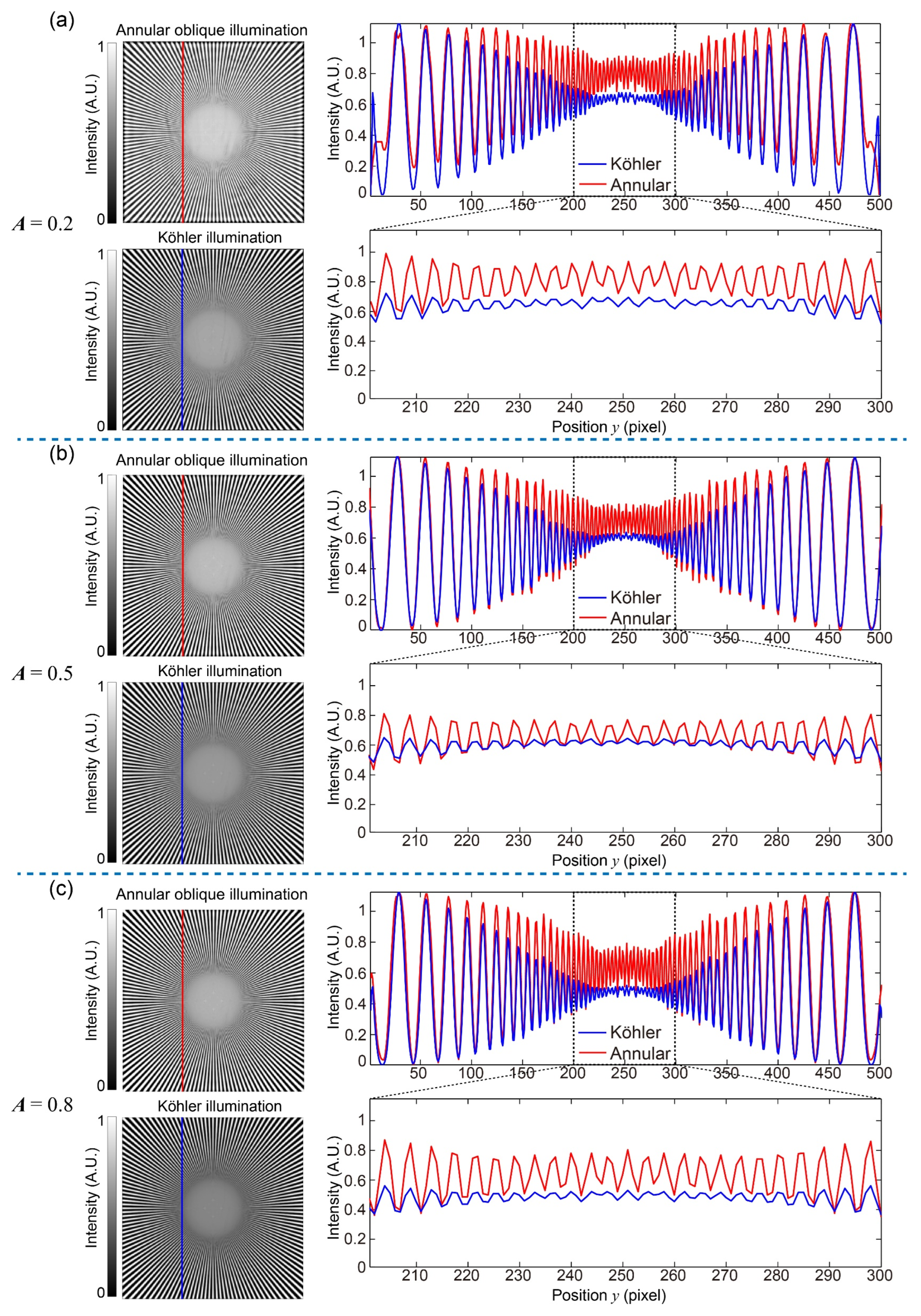
2.2. Unsymmetrical Interference

Here, we only consider the contrast related to the absorption because the phase contrast will vanish due to the incoherent superposition. According to Equation (1), we simulate an image formed by symmetrical and unsymmetrical diffraction orders in Figure 3. In the simulation, the impulse function $\delta \left(x,y\right)$ is used as the diffraction order. The ratio of amplitude distributions of the diffraction orders A₋₁, A₀, A₊₁ is 1:2.4:1, and that of B₀, B₊₁, and B₊₂ is 2.4:1:1. Figure 3a show the interference fringe formed by symmetrical diffraction orders: A₀, A₋₁, and A₊₁; Figure 3b shows the interference fringe formed by unsymmetrical diffraction orders: B₀ and B₊₁; Figure 3c show the interference fringe formed by unsymmetrical diffraction orders B₀, B₊₂. As can be seen in Figure 3a,b, the interference fringes have same spatial frequency, but the contrast in Figure 3b is relatively low. In Figure 3c, the spatial frequency of the fringe is higher.

The quantized contrast can be calculated by the formula [3]:

$$M_{\mathrm{contrast}}=\frac{I_{\max }-I_{\min }}{I_{\max }+I_{\min }},$$

(4)

where $I_{\max }$ is the maximal value of intensity, and $I_{\min }$ is the minimal value of intensity. According to Equation (4), the contrasts of Figure 3a–c are 1, 0.5, and 0.5, respectively. In the case of unsymmetrical interference, the contrast loss is 50%. In general, the high-frequency (high-resolution) information in the image is formed by unsymmetrical diffraction orders. This indicates that the contrast of sample details with high frequencies is lower than that with low frequencies.

2.3. Incoherent Superposition

According to Abbe’s theory, the image is an incoherent superposition of interference fringes in bright-field microscopy. As discussed above, high spatial-frequency interference fringes generally have a relatively low contrast. Therefore, in the incoherent superposition, the high-resolution information is suppressed by low spatial-frequency interference fringes formed by symmetrical diffraction orders. Finally, the high-resolution information may become non-structured intensities (or false light). This leads to the image suffering from the stray light [2].

For annular oblique illumination, the incoherent superposition of interference fringes (formed by unsymmetrical diffraction orders) only leads to a low intensity distribution, but the high-resolution information is not strongly suppressed. Therefore, by using image processing, the image contrast can be improved.

Köhler illumination or annular oblique illumination can be expressed as an incoherent superposition of a series of plane waves: $\exp \left[ju\left(\alpha ,\theta \right)\cdot x+jv\left(\alpha ,\theta \right)\cdot y\right]$ with the wave vector $\left[u\left(\alpha ,\theta \right),v\left(\alpha ,\theta \right)\right]$, where $\alpha$ and $\theta$ are the incident angle and the illumination azimuth angle; the thin sample can be described by the complex function $O\left(x,y\right)=T\left(x,y\right)\cdot \exp \left[j\varphi \left(x,y\right)\right]$; $T\left(x,y\right)$ is related to the transmittance; $\varphi \left(x,y\right)$ denotes the phase; the object wave can be described by $O\left(x,y\right)\exp \left[ju\left(\alpha ,\theta \right)\cdot x+jv\left(\alpha ,\theta \right)\cdot y\right]$. The image under oblique illumination can be written as

$$I_O\left(x,y;\alpha ,\theta \right)={\left|\left\{O\left(x,y\right)\exp \left[ju\left(\alpha ,\theta \right)\cdot x+jv\left(\alpha ,\theta \right)\cdot y\right]\right\}\otimes p\left(x,y\right)\right|}^2,$$

(5)

where $p\left(x,y\right)$ is the pupil of the system. The image under annular illumination at the largest angle of ${\alpha }_{\max }$ can be written as an incoherent superposition:

$$I_A\left(x,y;{\alpha }_{\max }\right)={\displaystyle {\int }_0^{2\pi }{I}_O\left(x,y;{\alpha }_{\max },\theta \right)d}\theta .$$

(6)

The image under Köhler illumination can also be written as an incoherent superposition:

$$I_K\left(x,y\right)={\displaystyle {\int }_0^{{\alpha }_{\max }}{\displaystyle {\int }_0^{2\pi }{I}_O\left(x,y;\alpha ,\theta \right)d}\theta d}\alpha .$$

(7)

In the bright-field microscopy, the sample is stained for imaging. We set $T\left(x,y\right)=\left\{1-A\left[1-t\left(x,y\right)\right]\right\}$, where $A$ is an absorption coefficient. To simulate a stained sample, $A$ is set to be 0.2, 0.5 and 0.8 (intensity absorptivity of 4%, 25% and 64%), respectively. A star-shaped resolution test target is used as $t\left(x,y\right)$ shown in Figure 4a; the phase $\varphi \left(x,y\right)$ is shown in Figure 4b.

In simulations, the number aperture of the objective lens ($N{A}_{obj}$) is set to be 0.7 (the incident angle of 34°). The illumination number aperture ($N{A}_{ill,\max }$) is set to be 0.56. For clarity, the magnification factor is set to be 1. The illumination wavelength $\lambda$ is 525 nm. The sampling interval is $\lambda /4$. The size of the simulated image is 500 × 500 pixels. Annular oblique illumination is simulated by using 120 plane waves with the wave vectors: $\left[u\left({\alpha }_{\max },{\theta }_1\right),v\left({\alpha }_{\max },{\theta }_1\right)\right]$, $\left[u\left({\alpha }_{\max },{\theta }_2\right),v\left({\alpha }_{\max },{\theta }_2\right)\right]$,…, $\left[u\left({\alpha }_{\max },{\theta }_{120}\right),v\left({\alpha }_{\max },{\theta }_{120}\right)\right]$. The interval angle of the azimuth angle $\theta$ is 3°. Köhler illumination is simulated by a superposition of 1000 plane waves with different wave vectors ($\left[u\left(\alpha ,\theta \right),v\left(\alpha ,\theta \right)\right]$ is at equal intervals, and $\sqrt{u^2\left(\alpha ,\theta \right)+v^2\left(\alpha ,\theta \right)}\le N{A}_{obj}/\lambda$) and the amplitude of the illuminating light wave is decreasing with the increase in incident angle, given by a multiple of $\cos \alpha$. The $N{A}_{ill}$ for Köhler illumination is also set to 0.56. When $A=0.2$, $A=0.5$ and $A=0.8$, the simulated images and their intensity distributions at the 170th column are also shown in Figure 5.

As shown in Figure 5, for Köhler-illuminated images, the overall contrast is high. However, the highest-frequency information almost vanishes, because in the incoherent superposition, the high-frequency information is obviously suppressed by low spatial-frequency information (corresponding to paraxial illumination). However, for annular oblique illumination without paraxial beams, the contrast of high-frequency information is well maintained. It is therefore beneficial to employ a normalization algorithm to improve the contrast. The normalized images are shown in Figure 6.

Compared to Köhler illumination, the image contrast for annular oblique illumination is enhanced obviously in Figure 6. To further increase the contrast, the blind deconvolution method was used [11,12]. The deconvoluted images are shown in Figure 7. By Equation (4), the quantized contrast is calculated in

Table 1. The contrast of 201 to 300 pixels at the 170th column in simulated images.

	Köhler Illumination			Annular Oblique Illumination
$A$	0.2	0.5	0.8	0.2	0.5	0.8
Figure 4 (raw image)	0.03	0.09	0.19	0.06	0.16	0.31
Figure 5 (normalized image)	0.15	0.15	0.22	0.29	0.32	0.43
Figure 6 (deconvoluted image)	0.19	0.24	0.24	0.37	0.49	0.50

.

In the simulated images, the contrast of 201 to 300 pixels at the 170th column is shown in Table 1. By image processing, the image contrast for annular oblique illumination was twice as high as that for Köhler illumination. When $A>0.5$, the contrast did not increase greatly.

2.4. Modulation Transfer Function (MTF)

For incoherent imaging, the PSF can easily be derived. The intensity in the image plane results from a convolution of the intensity in the object plane $I_{obj}\left(x,y\right)={\left|O\left(x,y\right)\right|}^2$ with the point spread function (PSF) $I_{PSF}\left(x,y\right)={\left|p\left(x,y\right)\right|}^2$. However, for partial coherent imaging, for example, in the simulation above, the PSF could only be approximately estimated by using a tiny object. Here, only one point (pixel) in $T\left(x,y\right)$ is set to 0, and the phase is ignored as a small strong absorption sample. The other parameters remained the same. The simulated sample, PSF, and MTF are illustrated in Figure 8. For the annular oblique illumination, the size of the PSF was smaller. Therefore, for annular oblique illumination, the MTF was wider than that for Köhler illumination. This explains how, for Köhler illumination, the contrast of high-frequency information will vanish faster.

3. Materials and Methods

The simplified configuration of the optical path with an annular oblique illumination is shown in Figure 9. In the experiment, we employed a standard transmission bright-field microscope (Nikon 80-i) with a Nikon 100X, $NA=1.25$ objective (oil immersion, plan achromat), and a CMOS camera (Andor, Zyla 4.2P, 6.5 μm Pixel size). The annular oblique illumination was created by an annular LED array, which consisted of 60 LEDs (central wavelength 520 nm, 10 nm bandwidth, and $\sim 25°$ divergence angle). The annular LED array was installed below the sample stage. Each LED illuminated the sample with the same incident angle of 65° ($N{A}_{ill}\approx 0.9$). For comparison, the $N{A}_{ill}$ of Köhler illumination was set to be 0.9 for a relatively good contrast, and a band-pass filter (central wavelength 520 nm, 10 nm band-pass regions) was used.

4. Results

We used a resolution target-USAF slide (Ready Optics, 2015a USAF) to show the contrast. The raw images, normalized images, and deconvolution images (10 iterations) are shown in Figure 10.

In the zoom-in areas, the quantized contrast of the pixels marked with solid lines is given. For the annular oblique illumination, the contrast of the high-frequency information was more significantly enhanced by image processing. Therefore, the highest distinguishable resolution target element for Köhler illumination was Element 3 in Group 11 (bar or space width 194 nm), whereas for the annular oblique illumination, the highest distinguishable resolution target element was Element 5 in Group 11 (bar or space width 154 nm).

We also demonstrated the proposed method on a skeletal-muscle cross-section slide (a stained educational prepared slide). The raw images, normalized images, and deconvolution images (20 iterations) are shown in Figure 11.

Compared to the resolution target, the biological sample had a complicated structure. It was difficult to separate high-frequency information for analysis in Figure 11. However, by image processing, the images for the annular oblique illumination became much clearer than those for the Köhler illumination, visually. This also proves that the proposed method can be used to enhance the contrast.

5. Discussion

Due to low-spatial frequency interference fringes (low-frequency information) formed by low diffraction orders, these orders will suppress high-frequency interference fringes (high-frequency information). The $N{A}_{obj}$ of the objective may affect the contrast. Here, we use parameters in Section 2.3 to simulate images with $N{A}_{obj}=0.3$ and $N{A}_{ill,\max }=0.3$ in Figure 12. The quantized contrast is shown in

Table 2. Contrast of 201 to 300 pixels at the 50th column in simulation images.

	Köhler Illumination	Annular Oblique Illumination
$A$	0.5	0.5
Figure 12a (raw image)	0.09	0.17
Figure 12b (normalized image)	0.24	0.48
Figure 12c (deconvoluted image)	0.24	0.49

.

As can be seen, the contrast of normalized images is high enough, and the contrast enhancement by deconvolution is minimal. This is because few high diffraction orders can pass the lens. The image formed by lower diffraction orders has a relatively high contrast. It can also be demonstrated by using an objective with $N{A}_{obj}=0.3$ in the experiment. The experiment results are shown in Figure 13.

6. Conclusions

In bright-field microscopy, Köhler illumination is the predominant technique for sample illumination. However, it cannot optimize the contrast and resolution simultaneously. In this paper, we discussed the main causes of contrast loss with Köhler illumination. We also combined LED annular oblique illumination with normalization and blind deconvolution to enhance the contrast. With the progress of optoelectronic devices, annular oblique illumination will prove more advantageous.

References

1. Wayne, R.O. Light and Video Microscopy, 2nd ed.; Academic Press: London, UK, 2013. [Google Scholar] [CrossRef]
2. Murphy, D.B.; Davidson, M.W. Fundamentals of Light Microscopy and Electronic Imaging, 2nd ed.; John Wiley & Sons: Hoboken, NJ, USA, 2013. [Google Scholar] [CrossRef]
3. Singer, W.; Totzeck, M.; Gross, H. Physical image formation. In Handbook of Optical Systems; Gross, H., Ed.; John Wiley & Sons: Weinheim, Germany, 2006; Volume 2. [Google Scholar] [CrossRef]
4. Mathews, W.W. The use of hollow-cone illumination for increasing image contrast in microscopy. Trans. Am. Microsc. Soc. 1953, 72, 190–195. [Google Scholar] [CrossRef]
5. Ma, X.; Zhang, Z.; Yao, M.; Peng, J.; Zhong, J. Spatially-incoherent annular illumination microscopy for bright-field optical sectioning. Ultramicroscopy 2018, 195, 74–84. [Google Scholar] [CrossRef] [PubMed]
6. Ma, X.; Zhou, B.; Su, Z.; Zhang, Z.; Peng, J.; Zhong, J. Label-free 3D imaging of weakly absorbing samples using spatially-incoherent annular oblique illumination microscopy. Ultramicroscopy 2019, 200, 97–104. [Google Scholar] [CrossRef] [PubMed]
7. Zuo, C.; Sun, J.; Li, J.; Zhang, J.; Asundi, A.; Chen, Q. High-resolution transport-of-intensity quantitative phase microscopy with annular oblique illumination. Sci. Rep. 2017, 7, 7654. [Google Scholar] [CrossRef] [PubMed]
8. Li, J.; Chen, Q.; Zhang, J.; Zhang, Y.; Lu, L.; Zuo, C. Efficient quantitative phase microscopy using programmable annular LED illumination. Biomed. Opt. Express 2017, 8, 4687–4705. [Google Scholar] [CrossRef] [PubMed] [Green Version]
9. Noda, T.; Kawata, S.; Minami, S. Three-dimensional phase contrast imaging by an annular oblique illumination microscope. Appl. Opt. 1990, 29, 3810–3815. [Google Scholar] [CrossRef] [PubMed]
10. Sanchez, C.; Cristóbal, G.; Bueno, G.; Blanco, S.; Borrego-Ramos, M.; Olenici, A.; Pedraza, A.; Ruiz-Santaquiteria, J. Oblique illumination in microscopy: A quantitative evaluation. Micron 2018, 105, 47–54. [Google Scholar] [CrossRef] [PubMed] [Green Version]
11. Holmes, T.J.; Bhattacharyya, S.; Cooper, J.A.; Hanzel, D.; Krishnamurthi, V.; Lin, W.; Roysam, B.; Szarowski, D.H.; Turner, J.N. Light Microscopic Images Reconstructed by Maximum Likelihood Deconvolution. In Handbook of Biological Confocal Microscopy; Pawley, J.B., Ed.; Springer: Boston, MA, USA, 1995; pp. 389–402. [Google Scholar] [CrossRef]
12. Holmes, T.J.; Biggs, D.; Abu-Tarif, A. Blind deconvolution. In Handbook of Biological Confocal Microscopy; Pawley, J.B., Ed.; Springer: New York, MA, USA, 2006; pp. 468–487. [Google Scholar] [CrossRef]
Figure 1. The optical path of Köhler illumination.
Photonics 10 00404 g001
Figure 2. The illustration of diffraction orders according to (a) the axial illumination, and (b) the largest-angle oblique illumination.
Photonics 10 00404 g002
Figure 3. Interference fringe formed by (a) symmetrical low diffraction orders, (b) unsymmetrical low diffraction orders, and (c) unsymmetrical high diffraction orders.
Photonics 10 00404 g003
Figure 4. The simulated sample, where (a) is the amplitude, and (b) is the phase.
Photonics 10 00404 g004
Figure 5. Simulated images: (a) A = 0.2 , simulated images with intensity distributions at the 170th column, and intensity distributions of 201 to 300 pixels at the 170th column; (b) A = 0.5 , simulated images with intensity distributions at the 170th column, and intensity distributions of 201 to 300 pixels at the 170th column; (c) A = 0.8 , simulated images with intensity distributions at the 170th column and intensity distributions of 201 to 300 pixels at the 170th column.
Photonics 10 00404 g005
Figure 6. Normalized images: (a) A = 0.2 , simulated images with intensity distributions at the 170th column, and intensity distributions of 201 to 300 pixels at the 170th column; (b) A = 0.5 , simulated images with intensity distributions at the 170th column, and intensity distributions of 201 to 300 pixels at the 170th column; (c) A = 0.8 , simulated images with intensity distributions at the 170th column and intensity distributions of 201 to 300 pixels at the 170th column.
Photonics 10 00404 g006
Figure 7. Deconvoluted images: (a) A = 0.2 , simulated images with intensity distributions at the 170th column, and intensity distributions of 201 to 300 pixels at the 170th column; (b) A = 0.5 , simulated images with intensity distributions at the 170th column, and intensity distributions of 201 to 300 pixels at the 170th column; (c) A = 0.8 , simulated images with intensity distributions at the 170th column and intensity distributions of 201 to 300 pixels at the 170th column.
Photonics 10 00404 g007
Figure 8. The simulated sample, PSF, and MTF, where (a) is a small strong absorption sample; (b) is the PSF for Köhler illumination; (c) is the PSF for annular oblique illumination; (d) is the cross section of MTF for Köhler illumination; (e) is the cross section of MTF for annular oblique illumination.
Photonics 10 00404 g008
Figure 9. The bright-field microscope with the annular LED array.
Photonics 10 00404 g009
Figure 10. The resolution target images: (a) is a raw Köhler-illuminated image, (b) is the normalized image of (a), (c) is the deconvoluted image of (b); (d) is a raw annular oblique-illuminated image, (e) is the normalized image of (d), (f) is the deconvoluted image of (e).
Photonics 10 00404 g010
Figure 11. Images of a skeletal-muscle cross-section slide: (a) is a raw Köhler-illuminated image, (b) is the normalized image of (a), (c) is the deconvoluted image of (b); (d) is a raw annular oblique-illuminated image, (e) is the normalized image of (d), (f) is the deconvoluted image of (e).
Photonics 10 00404 g011
Figure 12. Simulated images: (a) simulated images with intensity distributions at the 50th column, and intensity distributions of 201 to 300 pixels at the 50th column; (b) normalized images of (a) with intensity distributions at the 50th column, and intensity distributions of 201 to 300 pixels at the 50th column; (c) deconvoluted images of (b) with intensity distributions at the 50th column and intensity distributions of 201 to 300 pixels at the 50th column.
Photonics 10 00404 g012
Figure 13. The resolution target images: (a) is a raw Köhler-illuminated image, (b) is the normalized image of (a), (c) is the deconvoluted image of (b); (d) is a raw annular oblique-illuminated image, (e) is the normalized image of (d), (f) is the deconvoluted image of (e).
Photonics 10 00404 g013