Delineating Regional BES–ELM Neural Networks for Studying Indoor Visible Light Positioning

Abstract

This paper introduces a single LED and four photodetectors (PDs) as a visible light system structure and collects the received signal strength values and corresponding physical coordinates at the PD receiving end, establishing a comprehensive dataset. The K-means clustering algorithm is employed to separate the room into center and boundary areas through the fingerprint database. The bald eagle search (BES) algorithm is employed to optimize the initial parameters, specifically the weights and thresholds, in the extreme learning machine (ELM) neural network, and the BES–ELM indoor positioning model is established by region to improve positioning accuracy. Due to the impact exerted by the ambient environment, there are fluctuations in the positioning accuracy of the center and edge regions, and the positioning of the edge region needs to be further improved. To address this, it is proposed to use the enhanced weighted K-nearest neighbor (EWKNN) algorithm based on the BES–ELM neural network to correct the prediction points with higher-than-average positioning errors, achieving precise edge positioning. The simulation demonstrates that within an indoor space measuring 5 m × 5 m × 3 m, the algorithm achieves an average positioning error of 2.93 cm, and the positioning accuracy is improved by 86.07% relative to conventional BP neural networks.

1. Introduction

With the quick development of mobile Internet, applications based on location services have garnered widespread attention. At present, the technology for obtaining outdoor location information has been more mature, and large indoor buildings are gradually increasing. Moreover, the need for indoor positioning solutions has been increasing swiftly. Over the past few years, advancements in indoor positioning have been widely applied across diverse sectors, such as urban development, healthcare, construction, and chemical engineering. In particular, the main applications in the construction field include emergency preparedness [1], intelligent energy control [2], control of heating, ventilation, and air conditioning systems [3], and occupancy monitoring [4]. Various indoor wireless positioning technologies have emerged, such as wireless networks, RFID, Bluetooth, ultra-wideband, ultrasound, and infrared technologies. Within this array of technologies, indoor positioning technologies based on infrared, ultrasonic, and ultra-wideband are more costly to implement, and indoor positioning systems leveraging wireless networks and radio frequency identification are susceptible to multipath effects and interference and therefore have lower positioning accuracy [5,6,7]. Visible light communication (VLC) technology is being recognized as a creative remedy, offering not only the functions of communication and lighting but also realizing indoor positioning. VLC is rapidly developing due to its eco-friendly nature, immunity to electromagnetic disturbances, and abundant spectrum resources. These characteristics make it a promising technology for advancing wireless communication systems and offering robust solutions to indoor positioning challenges. Visible light positioning provides advantages such as high sensitivity and tolerance to electromagnetic interference and is suitable for hospitals, coal mines, airports, and other areas sensitive to electrical measurements [8,9].

Traditional VLC positioning methods consist of the time difference of arrival, time of arrival, angle of arrival, and received signal strength (RSS). Among these, RSS-based positioning methods are simple to implement and do not require complex equipment. Therefore, they have become a widely adopted approach in visible light indoor positioning [10]. Academics have integrated machine learning methods into visible light indoor positioning to enhance performance. Some of the commonly used machine learning methods for visible light indoor positioning are clustering, synthetic neural networks, and the fusion of several classifiers [11,12,13]. Sejan conducted an in-depth study of VLC techniques in multi-input multi-output communication environments and considered machine learning methods for multi-input multi-output VLC [14]. Previous VLC-based studies ignore reflections from ceilings, walls, indoor objects, etc., leading to positioning outcomes that are overly idealized and significantly divergent from real-world scenarios. Aminikashani illustrated the impact of reflections on several paths, with the central region of the room being virtually unaffected compared to the corners and edges, which yielded a poor effect [15]. It has been shown [16] that implementing a clustering algorithm prior to positioning, where the nearest point is queried within a single designated area, results in a shorter total execution time as well as a high positioning accuracy. Saadi employed just two LEDs along with the K-means algorithm for clustering, achieving a mean positioning error of 31 cm, marking the highest accuracy recorded in a realistic environment involving the use of LEDs [17]. Ren designed a hybrid positioning algorithm based on an extreme learning machine and density-based spatial clustering of noise applications (DBSCAN). Simulation results show that a neural network indoor visible light positioning algorithm combined with a clustering algorithm can effectively improve the positioning accuracy near indoor walls and corners [18]. Xu Yan proposed a multi-layer ELM-based subarea visible light indoor positioning algorithm that partitions the positioning area based on the size positioning error and the distribution characteristics and established a multi-layer limit learning machine to effectively minimize the positioning error within the boundary area [19].

Currently, there is limited research on the problem of large positioning errors within edge areas in the existing indoor visible light positioning technologies. Low accuracy in edge areas leads to a large average positioning error. In summary, to deal with the large positioning error in edge areas, this study suggests an algorithm for indoor visible light positioning according to the regional BES–ELM neural network. The K-means algorithm is first utilized to divide the room to be measured into regions. Given that the ELM neural network incline becomes trapped in local optima and exhibits slow convergence, the vulture search algorithm is utilized to refine the starting weights and ELM model thresholds. The algorithm imitates the strategy of vultures finding prey, combining the characteristics of random search and step-by-step optimization with the goal of effectively searching and converging to the optimal solution. The BES algorithm is suitable for solving nonlinear, non-convex, and other complex optimization problems due to its unique search strategy and global optimization ability. The trained BES–ELM neural network predicts the coordinates of the points to be measured, and then the EWKNN algorithm is employed to rectify the predicted points with an edge region positioning error larger than the mean positioning error, realizing accurate edge positioning and reducing the overall positioning error. Compared with the traditional indoor visible light positioning method, this paper improves the positioning accuracy of the central area and at the same time proposes to correct the edge area to address the problem of large positioning errors in the edge area, thereby improving the overall positioning accuracy.

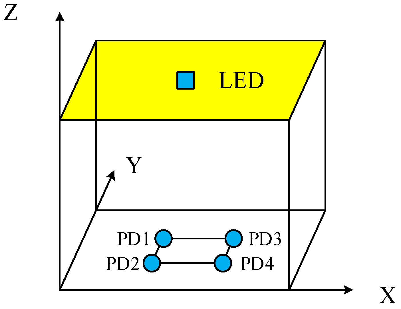
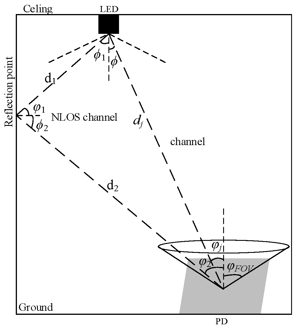
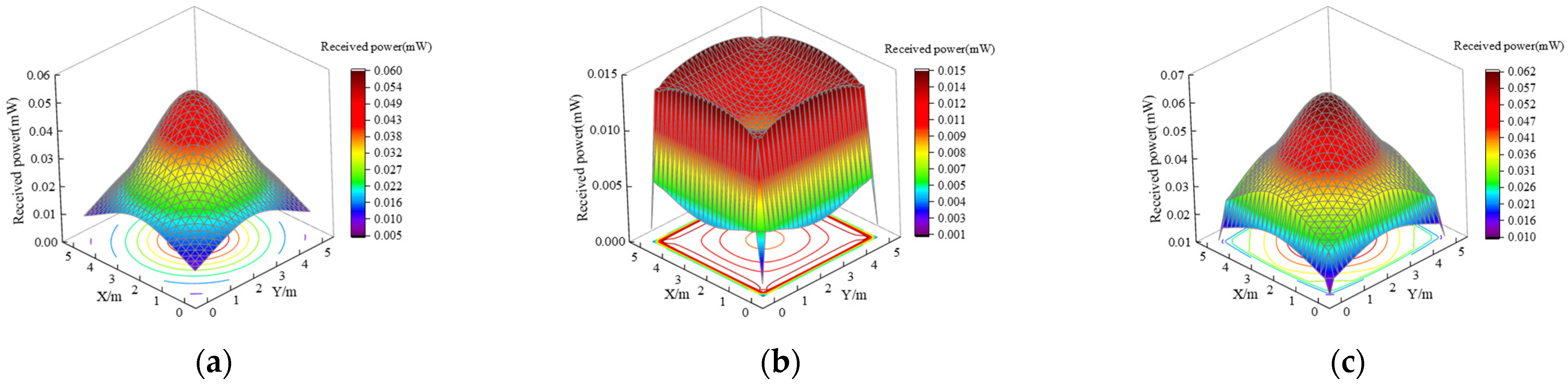
2. Indoor Model

Figure 1 illustrates the indoor VLC system model. An LED lamp is centrally positioned at the top of the room, functioning as the transmitter, the receiver is shaped as a square, the four PDs are located in the four corners of the receiver, and the position to be measured is located in the center of the receiver.

Figure 2 depicts the visible light transmission link. Under the assumption that the LED light source follows the Lambertian model, the straight line of sight (LOS) link channel gain H_LOSj in this study can be expressed as [20]:

$${H_{LOS}}_j=\left\{\begin{array}{c}{\displaystyle \frac{(m+1)A_r{\cos }^m(\varphi )\cos ({\phi }_j)}{2\pi {\mathrm{d}}_j^2}}\mathrm{T}(\phi \left)\mathrm{g}\right(\phi ) 0\le {\phi }_j\le {\phi }_{FOV}\\ 0\hspace{1em}\hspace{1em}\hspace{1em}\hspace{1em}\hspace{1em}\hspace{1em}\hspace{1em}\hspace{1em}\hspace{1em}\hspace{1em}\hspace{1em}\hspace{1em}\hspace{1em}{\phi }_j>{\phi }_{FOV}\hfill \end{array}\right.$$

(1)

where Ar represents the PD receiver effective receiving area; d_j represents the distance separating the receiving PD_jfrom the LED light source; φ_j represents the incidence angle of the receiving PDj; ϕ represents light source emission angle; φ_FOV represents the field-of-view angle of the receiver; m represents the Lambertian radiant order; T(φ) represents the optical filter gain, and g(φ) represents the optical concentrator gain, which can be expressed as:

$$g(\phi )=\left\{\begin{array}{c}{\displaystyle \frac{n^2}{{\sin }^2\left({\phi }_{\mathrm{FOV}}\right)}}\hspace{1em}0\le {\phi }_j\le {\phi }_{\mathrm{FOV}}\\ 0\hspace{1em}\hspace{1em}\hspace{1em}{\phi }_j>{\phi }_{\mathrm{FOV}}\end{array}\right.$$

(2)

where n is the receiver lens refractive index.

Presuming that the wall is made up of multiple diffuse mirrors with an area ∆A and reflectivity R_W, the channel gain for the non-line-of-sight (NLOS) channel is obtained using the following formula [22]:

$$H_{NLOSj}=\left\{\begin{array}{l}\sum _{\mathrm{Wall}}{\displaystyle \frac{A_{\mathrm{r}}\Delta A{R}_{\mathrm{W}}(m+1)}{2{\pi }^2{d}_1^2{d}_2^2}}{\cos }^m\left({\varphi }_1\right)\cos \left({\phi }_1\right)\cos \left({\varphi }_2\right)\cos \left({\phi }_2\right)T\left({\phi }_2\right)g\left({\phi }_2\right)\hspace{1em}0\le {\phi }_2\le {\phi }_{\mathrm{FOV}}\\ 0\hspace{1em}\hspace{1em}\hspace{1em}\hspace{1em}\hspace{1em}\hspace{1em}\hspace{1em}\hspace{1em}\hspace{1em}\hspace{1em}\hspace{1em}\hspace{1em}\hspace{1em}\hspace{1em}\hspace{1em}\hspace{1em}\hspace{1em}\hspace{1em}\hspace{1em}\hspace{1em}\hspace{1em}\hspace{1em}\hspace{1em}\hspace{1em}\hspace{1em}\hspace{1em}\hspace{1em}\hspace{1em}\hspace{1em}\hspace{1em}\hspace{1em}{\phi }_2>{\phi }_{\mathrm{FOV}}\hfill \end{array}\right.$$

(3)

where d1 and d2 are the distances; φ1 and φ2 are the angles of incidence; ϕ1 and ϕ2 are the irradiance angles; R_W indicates the wall’s reflectivity; and ∆A represents the area element at the reflective point on the wall.

The overall channel gain within the communication environment can be expressed as [23]:

$$H_j=H_{LOSj}+H_{NLOSj}$$

(4)

$$P_{rj}=P_t{H}_j$$

(5)

where Prj represents the received power and P_t represents the emitted power of the LED.

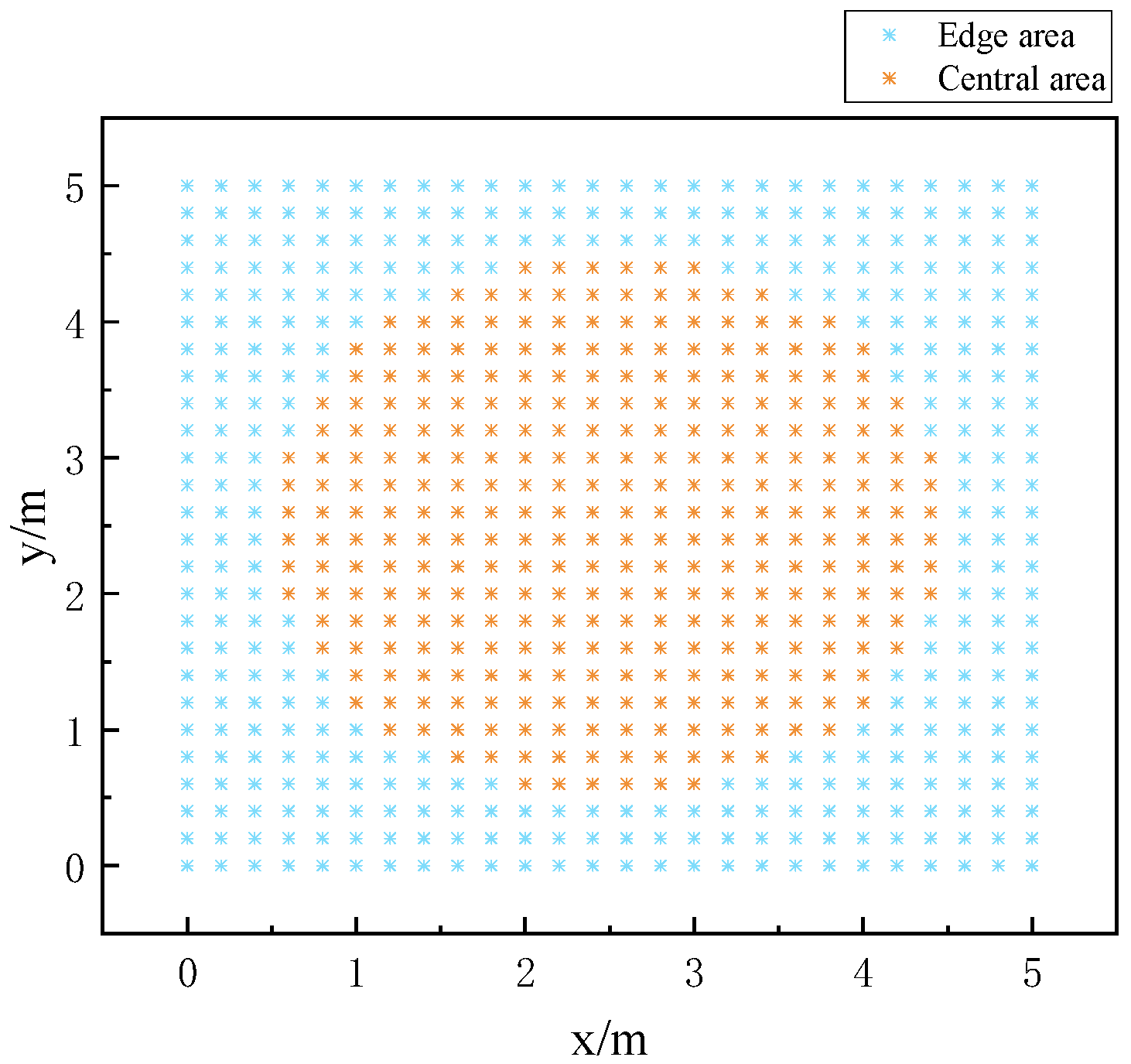
3. Delineating Regional Positioning

3.1. Create a Fingerprint Dataset

The fingerprint dataset is established by dividing the measurement plane into n² equally spaced grids, forming (n + 1)² grid points that serve as reference points. The optical power measured by the receiver PD_n (n = 1, 2, 3, 4) at each reference point is measured separately, and the measured optical power data at each reference point and the corresponding physical coordinates are stored to form the fingerprint dataset. f reference point fingerprint data are represented as [24]:

$$G_f=(x_f,y_f,P_{f1},P_{f2},P_{f3},P_{f4})$$

(6)

where P_fn (n = 1, 2, 3, 4) represents the optical power received by receiver n at the f reference point, and x_f, y_f are the horizontal and vertical coordinates of the f reference point, respectively. The fingerprint dataset built up from (n + 1)² reference points on the plane is denoted as:

$$H_f={[G_1,G_2,G_3,\cdots ,G_{{(n+1)}^2}]}^{\mathrm{T}}$$

(7)

3.2. K-Means Clustering Algorithm

The room boundary area is influenced by the surrounding environment, resulting in poor positioning stability and low accuracy. To improve positioning accuracy in the boundary area, the K-means clustering algorithm is used, using the received signal strength from the PD to divide the room into regions, thereby achieving precise regional positioning. The K-means algorithm proceeds as follows:

• Initialization. First, let t = 0, randomly select k sample data points as the center of the initial clustering, denoted as m(0) = (m1(0), …, ml(0), …, mk(0)).
• Clustering samples. For the set class center m(t) = (m1(t), …, ml(t), …, mk(t)), the corresponding ml(t) is the center of the lth class Cl. Calculate the distance of each data sample to the class center and allocate it to the nearest class center corresponding to the sample. The clustering results are formed, denoted as C(t).
• Determine the new center of classes. Based on the clustering result C(t) in the previous step, calculate the average value of all sample data in each current class, and use the obtained average value as the new center of mass, which is expressed as the following sequence: m(t + 1) = (m1(t + 1), …, ml(t + 1), …, mk(t + 1)).
• Re-allocation. Recalculate the distance of all sample data to the new class center and assign the data to the class represented by its nearest center.
• Iterate to end clustering. If the iteration converges (all the class centers no longer change) or the stopping condition is satisfied, output C* = C(t) at this point; otherwise, set t = t + 1 and return to Step Three.

3.3. BES Algorithm

A Malaysian scholar, H, proposed the BES algorithm (A Alsattar [25]). This algorithm possesses robust global search abilities and can efficiently address several intricate numerical optimization challenges. The BES algorithm emulates the hunting behavior of the bald eagle, structured into three distinct phases: selecting the search area, locating the prey within the search zone, and executing a dive to capture the prey [26].

The algorithm’s flow is shown as follows:

• Selecting the search space: The vulture randomly identifies a search area and assesses the prey quantity to find the optimal position, which facilitates the search for prey, and the update of the vulture’s position P_i,new in this stage is calculated by multiplying the a priori information of the upcoming search by α. This behavior is mathematically modeled as:

  $$P_{i,new}=P_{best}+\alpha \times r(P_{mean}-P_i)$$

  (8)

  where α represents the parameter for controlling position changes, with a range set between 1.5 and 2; r represents a randomly selected value within the range of 0 to 1; P_best is the best position for a search determined by the current bald eagle search; P_mean represents the mean distribution position upon the conclusion of the prior search; and P_i denotes the position of i bald eagle;

2.

Searching the space for prey. Bald eagles fly in a spiraling pattern in the chosen search area, hastening the search for prey and identifying the optimal position for a diving capture. Bald eagle locations are updated as follows:

$$P_{i,new}=P_i+x\left(i\right)\times \left(P_i-P_{mean}\right)+y\left(i\right)\times \left(P_i-P_{i+1}\right)$$

(9)

where x(i) and y(i) indicate the position of the bald eagle in polar coordinates, with the values ranging from (−1, 1).

3.

Dive to capture prey. From the optimal position inside the search area, bald eagles rapidly descend upon the target prey, while the remaining populace converges on the best location and launches an attack. The bald eagle’s position when swooping in a line can be shown as follows:

$$\left\{\begin{array}{c}{\delta }_x=x1\left(i\right)\times \left(P_i-c_1\times P_{mean}\right)\\ {\delta }_y=y1\left(i\right)\times \left(P_i-c_2\times P_{best}\right)\end{array}\right.$$

(10)

$$P_{i,new}=rand\times P_{best}+{\delta }_x+{\delta }_y$$

(11)

where c1 and c2 denote the bald eagle’s movement strength towards the optimal position as opposed to the central position, both taking values of (1, 2); rand represents a randomly generated value within (0, 1).

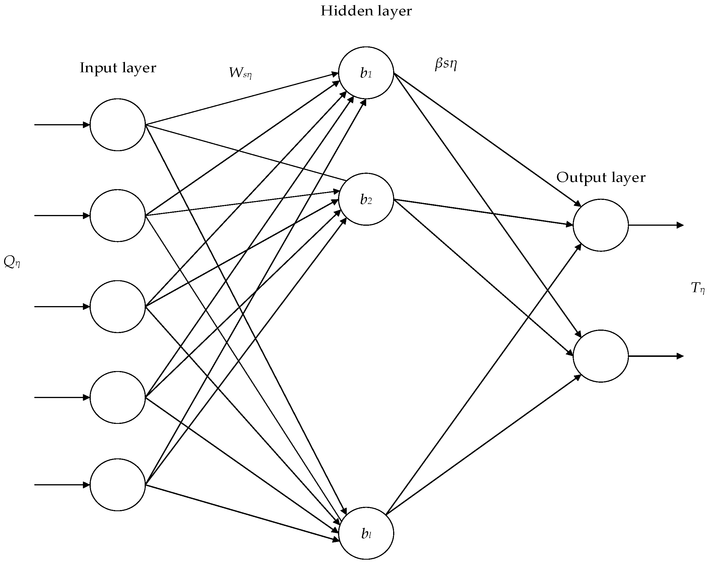
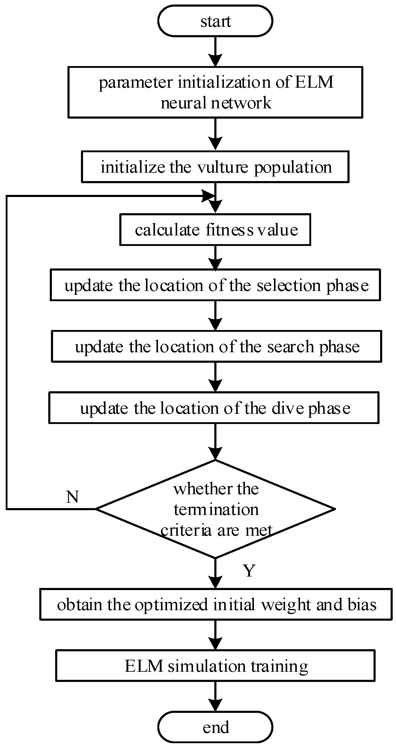
3.4. Modeling the BES–ELM

An extreme learning machine (ELM) is made up of three layers: input, hidden, and output [27]. The ELM algorithm randomly initializes the connection values and thresholds of the hidden layer without complex parameter settings, and the algorithm offers the benefits of reduced training parameters, faster training, and stronger generalization performance. The structure is depicted in Figure 3. The RSS value of the reference point is used as input for the ELM neural network to predict the coordinates of the reference point.

The mathematical expression for the ELM neural network is:

$${\mathit{T}}_{\eta }={\displaystyle \sum _{s=1}^L{\beta }_s}g\left(W_s\cdot Q_{\eta }+b_s\right),\eta =1,\cdots ,\tau$$

(12)

where Qη serves as the input matrix; βs denotes the weight matrix linking the s neuron in the hidden layer–output layer; bs denotes the threshold matrix of the hidden layer; τ is the total number of reference points; g(x) is the activation function; L denotes hidden layer neuron quantity; and Tη is the output matrix.

BES is used to optimize the initial weight thresholds of ELM random generation, and the initial weight thresholds of ELM are mapped to the location of each bald eagle across different dimensions. The fitness score of the entire bald eagle population is determined as the fitness function:

$$E={\displaystyle \frac{1}{n}}{{\displaystyle \sum _{s=1}^n\left(T_s-{\widehat{T}}_s\right)}}^2$$

(13)

where T represents the actual coordinates of the training set; $\widehat{T}$ represents the predicted coordinates; and n represents the whole quantity of training samples.

Therefore, identifying the best starting parameters for the neural network involves minimizing the adaptation value. The algorithm flow of BES–ELM is shown in Figure 4. It primarily comprises three parts: initialization of ELM neural network parameters, a BES optimization search to determine neural network parameters, and ELM neural network training.

The exact steps of implementation are as follows:

• Construct the network model. Initialize the model parameters and define the spatial dimensions of individual vultures by the number of input weights and thresholds within the network’s hidden layer.
• Calculate the fitness value of the algorithm using Equation (13). The optimal individual value is then updated based on the fitness obtained, with selection, searching, and swooping performed until the constraints are satisfied and the update is terminated to obtain the optimal solution.
• Train the network model. The parameter value that minimizes the fitness function is employed as the optimal weight threshold for the ELM network, which is then used to construct the BES–ELM network model.

3.5. Edge Area Correction

The weighted K-nearest neighbor algorithm involves determining the distance between the fingerprint data label at the current measurement point and every data label in the database [28]. It then sorts these distances, finds the k reference points that are closest to the data labels of the current measurement point, allocates weights to the positions of the k reference points, performs a weighted summation, and then averages the coordinates assigned to the weights to determine the current measurement point’s location. When the value of k is fixed, distant reference points may be included in the weight calculation, negatively impacting positioning accuracy. In this study, the enhanced weighted K-nearest neighbor algorithm is chosen to correct the predicted position of the edge region. The improved weighted K-nearest neighbor algorithm functions as a filter based on the weighted K-nearest neighbor algorithm by adding a threshold, and the value of k is selected dynamically.

According to the above description, after obtaining the forecasted position coordinates of the test point Z_A and the average error in positioning as predicted by the BES–ELM neural network is calculated, all the points to be tested Z_B in edge regions where the positioning error surpasses the mean positioning error are identified and the coordinates of the points to be tested Z_B are predicted using EWKNN. Let the optical power of Z_B be U_B = [P_B1, P_B1, P_B3, P_B4]^T and the optical power of the reference point Z_i be U_i = [P_i1, P_i1, P_i3, P_i4]^T.

The EWKNN algorithm flow is as follows:

• Calculate the Euclidean distance of Z_B from the optical power of all reference points d_i.

$$d_i=\sqrt{{\left(U_B-U_i\right)}^2},i=1,2,3\cdots ,{(n+1)}^2$$

(14)

2.

The obtained N Euclidean distances d_i are sorted in order of ascension to identify the mean E_d.

$$E_{\mathrm{d}}={\displaystyle \frac{{\mathrm{d}}_1+{\mathrm{d}}_2+\cdot \cdot \cdot +{\mathrm{d}}_N}{N}}$$

(15)

3.

Comparing each distance value d_i with the mean value E_d and removing distances higher than the average value, the number of remaining reference points is denoted as K.

4.

Continue the process described above, progressively decreasing the value of K as it approaches the true value. Select the remaining K reference points with the smallest Euclidean distance to assign weights to determine the coordinates of the points to be measured.

$$w_i={\displaystyle \frac{1/d_i}{{\displaystyle \sum _{i=1}^{K}1/d_i}}}$$

(16)

$$(x,y)={\displaystyle \sum _{i=1}^K{w}_i\ast (x_i,y_i)}$$

(17)

where w_i is the weight corresponding to the first K reference points; (x, y) represents the Z_B coordinates of the point to be measured; and (x_i, y_i) denotes the reference marker’s position coordinates.

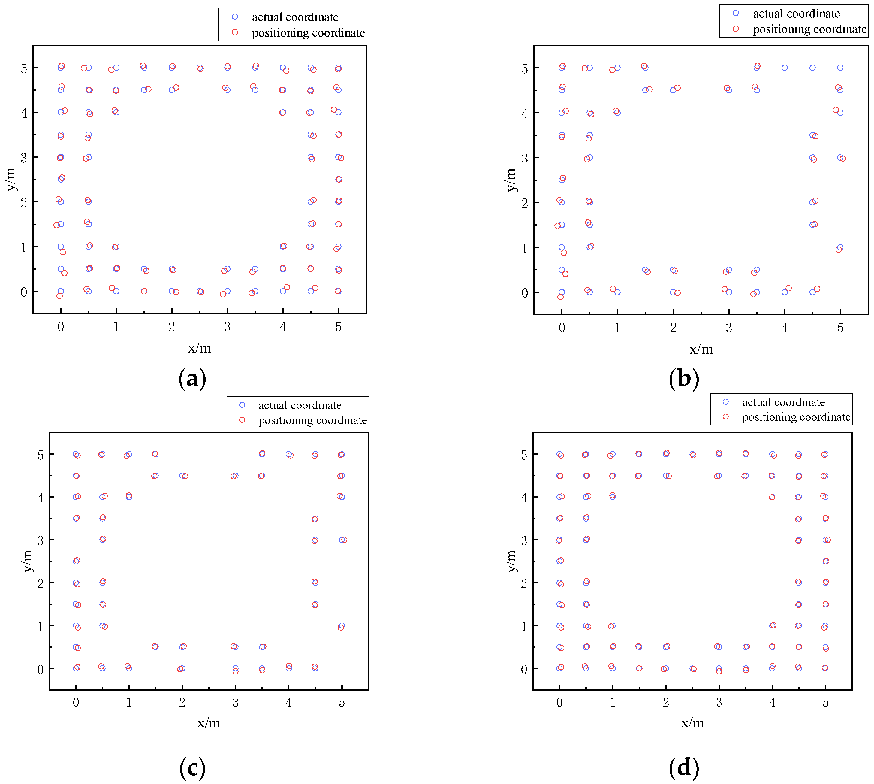
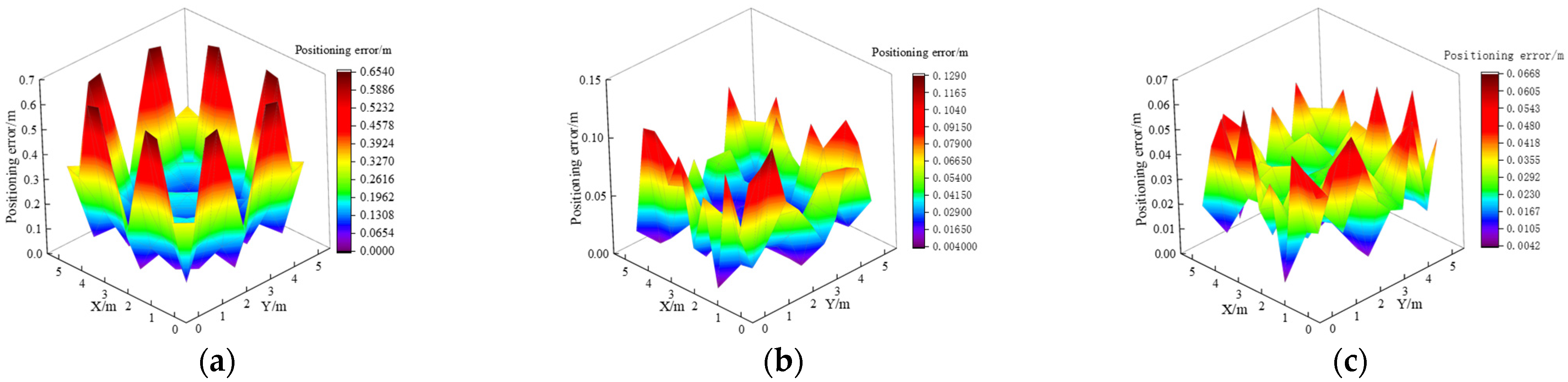
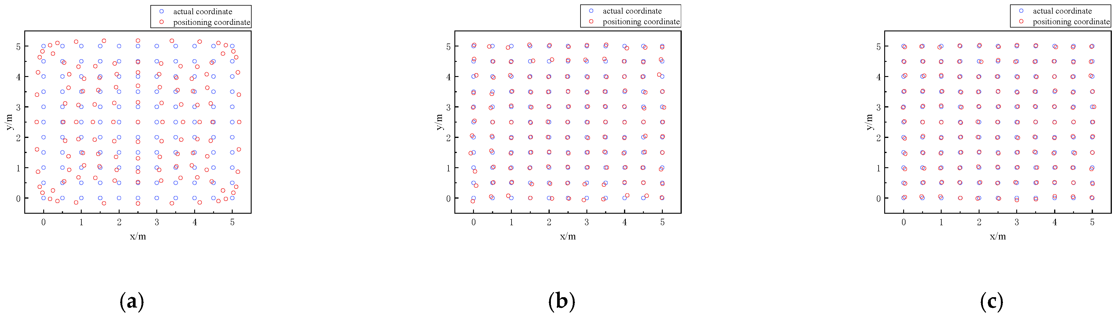
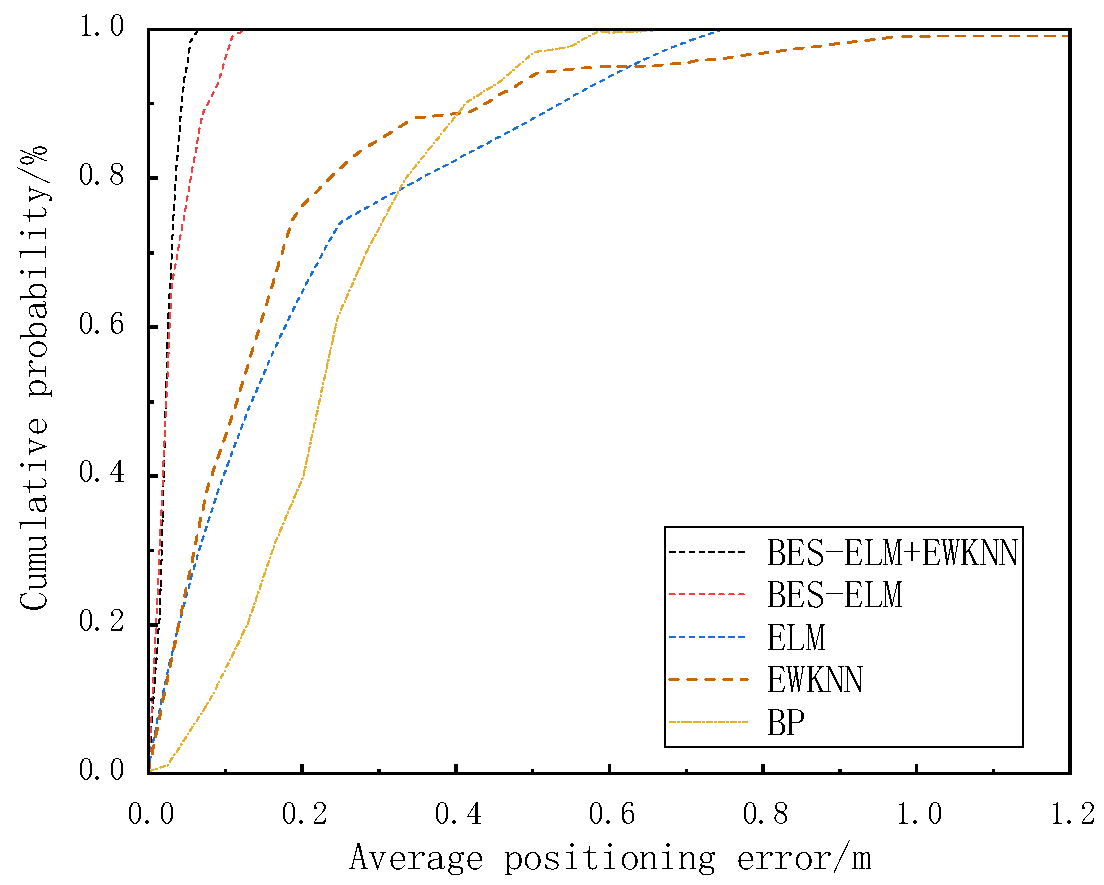
4. Simulation and Result Analysis

The room model measures 5 m × 5 m × 3 m, with an LED light mounted on the top of the room with coordinates (2.5 m, 2.5 m, 3 m). The measurement plane was uniformly divided into 25 × 25 small grids, creating 26 × 26 grid points. The receiver measured the optical power at each reference point, and the distance between the four horizontal PDs on the receiver and the receiver’s center had a 10 cm reference point. The primary simulation parameters are presented in

Table 1. VLP system simulation parameters.

Simulation Parameter	Simulation Value
LED emission power Pt	1 W
The actual receiving area of a single PD	1 cm2
Wall reflectivity RW	0.7
Receiver field of view φFOV	70°
The refractive index of the lens n	0.8
Optical concentrator gain g(φ)	1.5
Optical filter gain T(φ) SNR ELM training algorithm Number of iterations Target error Search Agents The BES max iteration	1 30 dB Gradient descent method 200 1 × 10−5 50 200

.

Considering both direct light from the LED and primary wall reflections, the receiver captures the optical power data at the reference location, and Figure 5 displays the dispersion of optical power.

The LOS channel captures the majority of the total optical power. Figure 5a illustrates the optical power distribution within the LOS channel, highlighting a pattern of higher intensity in the central region and lower intensity toward the edges. In Figure 5b, the optical power distribution for the NLOS channel is depicted, which shows that the reflected portion of the optical power is mainly concentrated in the edge region of the room to be tested, and the center region receives a low optical power intensity. Figure 5c shows the total received optical power distribution. In comparison to Figure 5a, the optical power distribution in the plane to be tested is gentler due to the inclusion of the NLOS channel.

Figure 5 illustrates a significant difference in the received signal’s quality between the boundary and the center region of the measurement plane, resulting in issues such as extended training time, large positioning errors in the boundary region, etc. The algorithm for K-means clustering is employed to divide the plane to be measured into regions based on the signal strength obtained at the reference point, and the positioning results of the edge region are corrected for the issue of significant errors in the edge region. The clustering results are shown in Figure 6.

The dataset contains information derived from the optical power readings captured by the receiver at the reference point, along with the corresponding horizontal and vertical coordinates of this point, and the data within the dataset are used as the training set. The BES–ELM neural network model is obtained via training. To validate the effectiveness of this algorithm, 121 uniformly selected points in the plane, which are to be tested as they are different from the reference points in the training set, are utilized as the test set. The optical power vectors corresponding to the test set points are utilized as inputs for the trained BES–ELM neural network to acquire the relevant predicted position coordinates (x_A, y_A). Assuming that the real coordinates of the point to be measured are (x_A1,y_A1), the mean positioning error predicted by the BES–ELM neural network is calculated after the error in positioning of the measurement point is determined. The points to be measured in the edge region are identified based on the clustering results, as illustrated in Figure 7a. Filter out all the to-be-tested points ZB in the edge region whose positioning error is larger than the mean positioning error, as shown in Figure 7b, and use the augmented-weighted K-nearest neighbor algorithm to correct them, as shown in Figure 7c, to obtain their final coordinates (x_B1, y_B1). Then, update the final corrected coordinates as the global locations of the to-be-tested points in the edge region, as seen in Figure 7d. The average positioning error in the edge region was 7.08 cm before correction and 3.87 cm after correction, reflecting a 45.33% improvement in positioning accuracy.

The simulation found that the amount of neurons within the layer that is hidden can directly influence the prediction accuracy of the neural network, which in turn affects the final positioning results. In order to identify the ideal number of neurons within the hidden layer, this research examines the mean positioning error of the ELM neural network across varying neuron quantities. Figure 8 illustrates the changes in the average positioning error as the quantity of neurons ranges from four to 24 in the hidden layer of the ELM neural network.

As illustrated in Figure 8, as the hidden layer’s neuronal count increases, the average positioning error decreases accordingly. As the hidden layer’s neuronal count increases, the learning time of the neural network becomes longer. Since the average positioning error does not change much after the hidden layer’s neuron count reaches 22, this study selects 22 neurons for the hidden layer of the ELM neural network. Once the hidden layer’s neuron count is configured to 22, the distribution of the ELM’s positioning error, the BES–ELM, and the BES–ELM corrected for the edges of the EWKNN is shown in Figure 9. The comparison of the position coordinates before and after correction is shown in Figure 10.

As shown in Figure 9, the peak positioning error for ELM is 65.40 cm, while BES–ELM exhibits a maximum error of 12.90 cm. The maximum positioning error of BES–ELM after EWKNN edge correction is 6.68 cm. From Figure 10, it is evident that the total positioning error of the ELM positioning plane is larger, and the edge region is especially obvious. The positioning accuracy of BES–ELM has been notably enhanced, and the positioning error of the edge region has been reduced compared with that of ELM. In addition, the EWKNN edge correction of the edge region of BES–ELM has been effectively corrected. The ELM exhibits an average positioning error of 23.79 cm, while BES–ELM achieves an average error of 4.15 cm. After edge correction, the average positioning error is further decreased to 2.93 cm. This algorithm’s positioning accuracy is increased by 82.55% compared to the ELM neural network, and by 29.39% compared to the BES–ELM algorithm.

In order to evaluate the suggested algorithm’s efficacy, a comparison of the localization mistakes’ cumulative distribution between this algorithm and the traditional method was performed, and the results are displayed in Figure 11. From Figure 11, it is evident that 90% of the positioning error of this paper’s algorithm is less than 4.53 cm for the ELM neural network, 90% of the location errors are less than 55.49 cm, errors less than 53.61 cm account for 90% of the KNN’s placement mistakes, errors less than 50.37 cm account for 90% of the WKNN’s placement mistakes, errors less than 44.74 cm account for 90% of the EWKNN’s placement mistakes, 90% of the positioning errors of the BP neural network are lower than 41.59 cm, and 90% of the positioning errors of the BES–ELM neural network are less than 8.72 cm.

The average positioning error using the suggested algorithm and conventional techniques is compared. According to

Table 2. Comparison of the various positioning methods’ positioning performance.

Algorithm	Average Positioning Error (cm)	Average Positioning Time(s)
BP	21.04	0.16358
ELM	23.79	0.18461
EWKNN	17.37	0.16694
BES–ELM	4.15	0.21847
BES–ELM + EWKNN	2.93	0.23961

, the proposed algorithm demonstrates superior positioning performance compared to conventional methods, effectively reducing the positioning error at the measured points. The method in this research enhances the location precision in comparison to the BP neural network by 86.07%, 87.68% compared to the ELM neural network, 84.17% compared to the EWKNN algorithm, and 29.39% compared to the unmodified BES–ELM algorithm. Compared with the BP neural network, ELM neural network, EWKNN, and BES–ELM, the average positioning time of the proposed algorithm is slightly longer. The average positioning time of the proposed algorithm alone is controlled within 1 s, which will not affect daily use.

5. Conclusions

This paper addresses the issue of poor edge region positioning accuracy in traditional indoor visible light positioning algorithms by proposing a regional BES–ELM neural network positioning algorithm with a single LED lamp to correct the edge region positioning results. By utilizing the K-means clustering algorithm to divide the area to be measured into the center region and the boundary area, establish the BES–ELM neural network indoor positioning model to predict the global area to be measured, screen out the points to be measured where the positioning error in the boundary region exceeds the mean positioning error, and use the EWKNN algorithm for the correction of the positioning error to realize the accurate positioning of edge areas and increase the precision of the positioning model’s global positioning. Compared to the conventional BP neural network algorithm, the precision of positioning is enhanced by 86.05%. Compared to the uncorrected BES–ELM neural network algorithm, the accuracy of positioning is enhanced by 29.39%, fulfilling the positioning service needs for the majority of indoor application scenarios.

The indoor environment discussed in this paper is relatively ideal, but changes in real-world applications may reduce the effectiveness of the fingerprint database, emphasizing the need for its maintenance and regular updates. In subsequent work, further optimization and improvement of the system should consider the selection of special positions to monitor the fluctuation of fingerprint data and facilitate the timely update of the dataset, as well as the integration of various positioning methods to address the limitations inherent in using a single technique.

References

- Filippoupolitis, A.; Oliff, W.; Loukas, G. Bluetooth Low Energy Based Occupancy Detection for Emergency Management. In Proceedings of the 2016 15th International Conference on Ubiquitous Computing and Communications and 2016 International Symposium on Cyberspace and Security (IUCC-CSS), Granada, Spain, 14–16 December 2016; pp. 31–38. [Google Scholar]
- Tekler, Z.D.; Low, R.; Yuen, C.; Blessing, L. Plug-Mate: An Iot-Based Occupancy-Driven Plug Load Management System in Smart Buildings. Build. Environ. 2022, 223, 109472. [Google Scholar] [CrossRef]
- Balaji, B.; Xu, J.; Nwokafor, A.; Gupta, R.; Agarwal, Y. Sentinel: Occupancy Based Hvac Actuation Using Existing Wifi Infrastructure within Commercial Buildings. In Proceedings of the 11th ACM Conference on Embedded Networked Sensor Systems, Roma, Italy, 11–15 November 2013; p. 17. [Google Scholar]
- Tekler, Z.D.; Chong, A. Occupancy Prediction Using Deep Learning Approaches across Multiple Space Types: A Minimum Sensing Strategy. Build. Environ. 2022, 226, 109689. [Google Scholar] [CrossRef]
- Zhao, C.; Zhang, H.; Song, J. Fingerprint-based indoor visible light positioning method. Chin. J. Lasers. 2018, 45, 202–208. [Google Scholar]
- Cao, Y.; Dang, Y.; Peng, X.; Li, Y. TOA/RSS hybrid information indoor visible light positioning method. Chin. J. Lasers 2021, 48, 133–141. [Google Scholar]
- Dong, W.; Wang, X.; Wu, N. A hybrid RSS/AOA based algorithm for indoor visible light positioning. Laser Optoelectron. Prog. 2018, 55, 88–93. [Google Scholar]
- Wang, R.; Niu, G.; Cao, Q.; Chen, C.S.; Ho, S.-W. A Survey of Visible-Light-Communication-Based Indoor Positioning Systems. Sensors 2024, 24, 5197. [Google Scholar] [CrossRef]
- Almadani, Y.; Ijaz, M.; Adebisi, B.; Rajbhandari, S.; Bastiaens, S.; Joseph, W.; Plets, D. An experimental evaluation of a 3D visible light positioning system in an industrial environment with receiver tilt and multipath reflections. Optics Commun. 2020, 483, 126654. [Google Scholar] [CrossRef]
- Ke, X.; Ding, D. Wireless Optical Communication, 2nd ed.; Science Press: Beijing, China, 2022. [Google Scholar]
- Huy, Q.T.; Cheolkeun, H. Improved Visible Light-Based Indoor Positioning System Using Machine Learning Classification and Regression. Appl. Sci. 2019, 9, 1048. [Google Scholar] [CrossRef]
- Raes, W.; Knudde, N.; De Bruycker, J.; Dhaene, T.; Stevens, N. Experimental Evaluation of Machine Learning Methods for Robust Received Signal Strength-Based Visible Light Positioning. Sensors 2020, 20, 6109. [Google Scholar] [CrossRef]
- Shu, Y.-H.; Chang, Y.-H.; Lin, Y.-Z.; Chow, C.-W. Real-Time Indoor Visible Light Positioning (VLP) Using Long Short Term Memory Neural Network (LSTM-NN) with Principal Component Analysis (PCA). Sensors 2024, 24, 5424. [Google Scholar] [CrossRef]
- Sejan, M.A.S.; Rahman, M.H.; Aziz, M.A.; Kim, D.-S.; You, Y.-H.; Song, H.-K. A Comprehensive Survey on MIMO Visible Light Communication: Current Research, Machine Learning and Future Trends. Sensors 2023, 23, 739. [Google Scholar] [CrossRef]
- Gu, W.; Aminikashani, M.; Deng, P.; Kavehrad, M. Impact of Multipath Reflections on the Performance of Indoor Visible Light Positioning Systems. J. Light. Technol. 2016, 34, 2578–2587. [Google Scholar] [CrossRef]
- Saadi, M.; Zhao, Y.; Wuttisttikulkij, L.; Tahir, M. A heuristic approach to indoor positioning using light emitting diodes. J. Theor. Appl. Inf. Technol. 2016, 2984, 332–338. [Google Scholar]
- Saadi, M.; Ahmad, T.; Zhao, Y.; Wuttisttikulkij, L. An LED Based Indoor Positioning System Using k-Means Clustering. In Proceedings of the 2016 15th IEEE International Conference on Machine Learning and Applications (ICMLA), Anaheim, CA, USA, 18–20 December 2016; pp. 246–252. [Google Scholar]
- Liu, R.; Liang, Z.; Yang, K.; Li, W. Machine learning based visible light indoor positioning with single-LED and single rotatable photo detector. IEEE Photonics J. 2022, 14, 7322511. [Google Scholar] [CrossRef]
- Xu, Y.; Wang, X. Indoor positioning algorithm of delineating regional visible light based on multilayer ELM. J. Hunan Univ. Nat. Sci. 2019, 46, 125–132. [Google Scholar]
- Ding, D.Q.; Ke, X.Z.; Li, J.X. Design and simulation on the layout of lighting for VLC system. Opto-Electr. Eng. 2007, 34, 131–134. [Google Scholar]
- Van, M.T.; Van Tuan, N.; Son, T.T.; Le-Minh, H.; Burton, A. Weighted k-nearest neighbor model for indoor VLC positioning. IET Commun. 2017, 11, 864–871. [Google Scholar] [CrossRef]
- Maheepala, M.; Kouzani, A.Z.; Joordens, M.A. Light-based indoor positioning systems: A review. IEEE Sens. J. 2020, 20, 3971–3995. [Google Scholar] [CrossRef]
- Ke, C.; Shu, Y.; Ke, X. Research on Indoor Visible Light Location Based on Fusion Clustering Algorithm. Photonics 2023, 10, 853. [Google Scholar] [CrossRef]
- Qin, L.; Zhang, C.; Guo, Y. Research on visible light indoor positioning algorithm based on Elman neural network. Appl. Opt. 2022, 42, 24–31. [Google Scholar]
- Alsattar, A.H.; Zaidan, A.A.; Zaidan, B.B. Novel meta-heuristic bald eagle search optimization algorithm. Artif. Intell. Rev. 2020, 53, 2237–2264. [Google Scholar] [CrossRef]
- Chhabra, A.; Hussien, A.G.; Hashim, F.A. Hashim. Improved bald eagle search algorithm for global optimization and feature selection. Alex. Eng. J. 2023, 68, 141–180. [Google Scholar] [CrossRef]
- Huang, G.-B.; Zhu, Q.-Y.; Siew, C.-K. Extreme learning machine: Theory and applications. Neurocomputing 2006, 70, 489–501. [Google Scholar] [CrossRef]
- Tran, H.Q.; Ha, C. Machine learning in indoor visible light positioning systems: A review. Neurocomputing 2022, 491, 117–131. [Google Scholar] [CrossRef]