Enhanced Thermoacoustic Imaging System with Parallel Ultrasonic Velocity Measurement for Distinguishing Types of Microwave-Absorbing Anomalies

Abstract

Microwave-absorbing suspicious objects (MASOs) found using microwave-induced thermoacoustic imaging (MTI) can be divided into two types—endogenous (such as tumors or hematoceles) and exogenous (such as calculi or foreign bodies). These have different microwave absorption or ultrasonic velocity than normal human tissue, so MTI is efficient in detecting these anomalies. However, the existing MTI techniques can only reflect morphological information, making it difficult to distinguish the type of each anomaly. In this paper, a newly enhanced MTI system composed of a multiple-element ring transducer and a parallel data acquisition system (DAS) is presented. By using ultrasonic velocity and microwave absorption measurements, where the ultrasonic velocity is mainly used as an additional parameter to reflect mechanical characteristics, the type of the detected anomaly can be identified. In our experiments, the MASO can be located through the absorption difference detected by MTI. Due to the use of multiple-element transducers and a parallel DAS, the raw data can be acquired within about 20 ms for a two-dimensional image. Additionally, the ultrasonic velocity of the MASO can be calculated from the time sequence diagram of ultrasound propagation with a maximum time error of 0.084 μs. Apart from distinguishing the type of the anomaly, the proposed ultrasonic velocity-assisted microwave-induced thermoacoustic imaging (US-MTI) system has other advantages, such as being noninvasive, and allowing rapid imaging and a large field of view, which make US-MTI a suitable modality for regular screening.

1. Introduction

Microwave-induced thermoacoustic imaging (MTI) is an emerging imaging modality that can determine the microwave absorption coefficient of biological tissue [1,2,3,4,5,6,7,8,9]. In the past few years, a large number of works have found that MTI can detect microwave-absorbing suspicious objects (MASOs) in biological tissue, particularly breast cancer tissues [10,11,12] and foreign objects [13,14] inside the body, up to a depth of a dozen centimeters. The development of pulsed microwave sources [15,16,17], ultrasonic detectors [11,12,18], and the data acquisition system (DAS) [12] has alleviated the bottleneck in hardware devices and will propel the method further towards clinical application. With the help of the ultra-short microwave pulse generator and a ring transducer array, our group designed a real-time MTI system dedicated to imaging deep breast tumors [16]. However, the microwave absorptivity distribution cannot reflect the microwave absorption coefficient quantitatively, and as a result, the existing MTI techniques can only determine morphological information. In other words, almost all types of MASOs display similar image features apart from their shapes. Therefore, the type of MASO cannot be identified from reconstructed MTI images unless additional parameters are introduced.

Different objects each have a different ultrasonic velocity, which reflects the viscoelasticity and mass density of the object and can, therefore, serve as an identification target. Ultrasonic velocity is also a key factor in MTI, as heterogeneous components can lead to image distortion. Several groups have reported reconstruction algorithms for MTI to compensate for acoustic speed heterogeneity [19,20,21]. In one study, a practical system based on a similar reconstruction algorithm was proposed to improve the imaging quality of MTI [22], rather than to identify types of MASOs. The system employs two single-element unfocused ultrasonic transducers with a 2.25 MHz main frequency. One transducer acts as a transmitter and the other is the receiver. Due to the large size (approximately 6 mm in diameter) and low main frequency, the measurement accuracy of the transducers is poor. Additionally, the rotation of the single-element transducers wastes a lot of time, and the complex imaging algorithm further worsens the situation.

Generally speaking, MASOs inside the human body can be divided into endogenous types (e.g., breast tumors) and exogenous types (foreign objects). Compared to normal tissue, they both have different microwave absorptions, so MTI is able to characterize their margins. However, this information is inadequate for medical staff to determine the next step—after all, not all MASOs need to be cleared or biopsied. In this paper, a newly developed MTI system composed of a multiple-element ring transducer and a parallel data acquisition system (DAS) is presented. As well as increasing the array element number to improve the detection sensitivity, we employed a smaller point sound source (0.1 mm iron needle) to improve the measurement accuracy (which will produce an ultrasound with a high signal-to-noise ratio under the excitation of pulsed microwaves). In our experimental system, MTI and sound speed measurement can be realized simultaneously in the same excitation system and data acquisition system. The ultrasonic velocity is acquired as an additional parameter to determine the category of the component of the MASO. The proposed ultrasonic velocity-assisted microwave-induced thermoacoustic imaging (US-MTI) system can be potentially used as an alternative foreign body-screening modality.

2. Model and Methods

2.1. Model

Consider an ultrasound beam with a certain frequency penetrating through samples with different layers, as shown in Figure 1. Each layer has a single ultrasonic velocity, and there is a clear boundary between the different layers. The transmission time is determined by the following equation:

$$\begin{array}{l}t={\displaystyle \underset{l_1}{\int }\frac{1}{v_1}ds}+{\displaystyle \underset{l_2}{\int }\frac{1}{v_2}ds}+\cdot \cdot \cdot \cdot \cdot \cdot +{\displaystyle \underset{l_{\mathrm{n}}}{\int }\frac{1}{v_{\mathrm{n}}}ds}\\ l_1+l_2+\cdot \cdot \cdot \cdot \cdot \cdot +l_{\mathrm{n}}=l\end{array}$$

(1)

where l_n is the thicknesses of layer n, v_n is the ultrasonic velocity in each of the n layers, and l is the total transmission length.

When there are only two layers and the outer material is deionized water, v_w and v_s represent the ultrasonic velocity in the water and in the sample, respectively. In this case, Equation (1) can be simplified as $t={\displaystyle \underset{h}{\int }\frac{1}{v_{\mathrm{s}}}ds}+{\displaystyle \underset{l-h}{\int }\frac{1}{v_w}ds}$, where l is the total transmission length, t is the transmission time calculated using the received ultrasonic signal, and h is the thickness of the sample. The parameters t, h, l, and v_w are known. The solution of the simplified equation is as follows:

$$v_s={\displaystyle \frac{h}{t-\frac{l-h}{v_w}}}.$$

(2)

2.2. Apparent Thickness and Actual Thickness

In the process of MTI image reconstruction, the parameter h may have significant calculation error due to the use of a uniform ultrasonic velocity. In other words, for a sample with a thickness h, the transmission time t_s is calculated as t_s = h/v_s; however, if a uniform ultrasonic velocity v_w is used in reconstruction, the apparent thickness in the MTI image will be h′ = hv_w/v_s. Therefore, the apparent thickness is usually not equal to the actual thickness and may blur or distort the image. When implementing the measured apparent thickness from thermoacoustic imaging, Equation (2) can be revised to the following:

$$v_s={\displaystyle \frac{v_{w}l+v_w{h}^{\prime }-{v_w}^{2}t}{h^{\prime }}}.$$

(3)

The apparent thickness h′ of the MASO is a critical parameter in the experimental suspicious area identification, which is obtained from the MTI image. The iterative steps of this method are summarized as follows: (a) fix ‘l’ and acquire the MTI signal and the time ‘t’ for the signal; (b) construct the MTI image using v_w; (c) obtain an estimate of h′ from the image; (d) use Equation (3) to obtain v_s from h′ and ‘t’; (e) use back projection as well as v_w and v_s to obtain the corrected image.

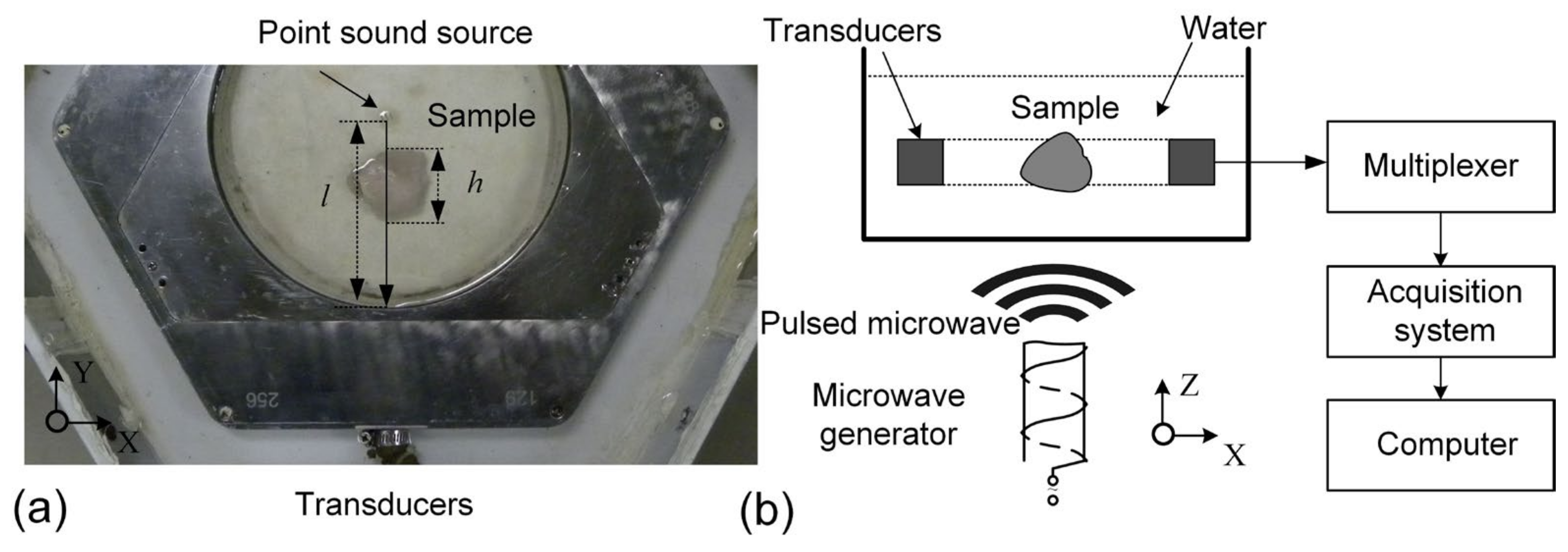
2.3. Experimental Setup

Based on the above assumptions, a US-MTI system was built. An image of the detection section is shown in Figure 2a, and a schematic diagram of the whole system is shown in Figure 2b. A Cartesian coordinate system (X, Y, Z) is used to describe the imaging scenario. A microwave generator (JH-100-40, Jiahai Co., Ltd., Changsha, China) with a main frequency of 450 MHz is used to transmit a 10 ns microwave pulse train (2~3 ns per pulse) at a max pulse repetition frequency of 100 Hz, which is controlled by a function generator. The central frequency of the 384-element full ring ultrasonic transducer (10C384-1.62*8-R100 AHA001, Doppler Ltd., Guangzhou, China) is 10 MHz, with a bandwidth of 70%. In this paper, only 1/3 of the full ring, shown in Figure 2a, is used in the US-MTI system. Further, a 0.1 mm iron needle is placed outside of the imaging region, serving as a point sound source. The h marked in Figure 2a is the width occupied by the measured sample on the ultrasound transmission path l, which can be indirectly obtained through MTI images. The transducer and the sample are immersed in water for the coupling of thermoacoustic signals. A 64-channel data acquisition system (DAS) [11,12] is used to transmit and acquire the raw MTI signals from the transducers. Afterward, the acquired signals are filtered and averaged using signal processing software on the computer. The DAS is triggered synchronously by the same function generator that is used to trigger the microwave generator. A signal frame is acquired and transmitted within 10 ms using the DAS. Finally, the signal amplitudes corresponding to each discrete point are used to reconstruct a 2D image using a back-projection algorithm [5], and at the same time, the ultrasonic velocity is calculated according to Equation (2). In this paper, all the measurements were done at room temperature (26 °C).

3. Results

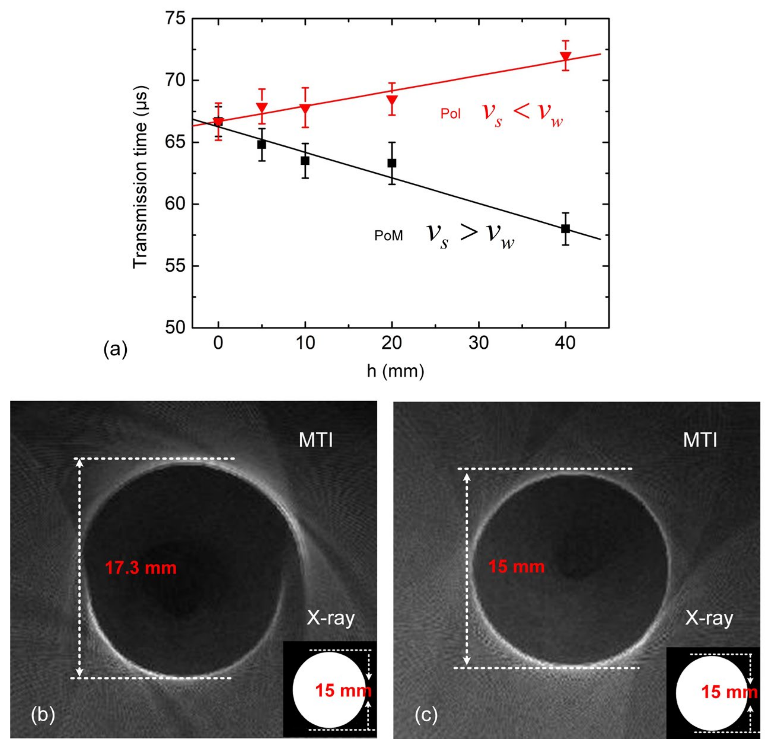
3.1. Influence of Non-Uniform Ultrasonic Velocity

When the parameters l and v_w are fixed, the parameter t will be linearly dependent on h, according to Equation (2). Moreover, when the ultrasonic velocity of the sample is smaller than that of water, the relationship between t and h is direct; otherwise it is a linear function with a negative slope. This relationship is verified by an experiment, as shown in Figure 3a. The velocity of ultrasound in Polyfoam (v_s) is less than that of water (v_w), and the velocity of ultrasound in Polymethyl methacrylate (v_s) is larger than that of water (v_w); therefore, as the sample thickness h increases, the Pol curve (transmission time) rises and the PoM falls. The ultrasonic velocity can be calculated using the proposed method, as long as the transmitted ultrasound is detectable, as shown in

Table 1. The velocity of ultrasound (Refs. [23,24,25,26,27,28]) for various materials.

Materials (26 °C)	Velocity of Ultrasound (SD) (m/s)
	Used in the Literature	Calculated by This Work
Softwood	523~590	545 (7)
Rubber	1152~1272	1182 (9)
Polyfoam	1285~1388	1328 (6)
Mineral oil	1322~1467	1337 (13)
Polyvinyl chloride	2329~2520	2388 (9)
Water	1511	1502 (5)
Fat	1468~1487	1469 (6)
Muscle	1568~1600	1586 (9)
Breast tumor	1470~1513	1510 (9)

The velocity of ultrasound (Refs. [23,24,25,26,27,28]). SD: standard deviation.

. The reference values of ultrasonic velocity for various materials are also shown in Table 1, and these are all quoted from the literature. In order to better illustrate this, an experiment was performed and the results are shown in Figure 3b. The sample used in the experiment was a rubber object with a diameter of 15 mm; the shape and size are shown in the X-ray image. Figure 3b,c were reconstructed by using 1/2 of a full ring transducer (1–192 elements) instead of the original signal. In the reconstructed image, the front arc has been accurately reconstructed; however, the arc in the opposite direction is larger than the actual size. The apparent thickness of this sample is approximately 17.3 mm rather than the actual 15 mm. As a comparison, the apparent thickness is approximately equal to the actual thickness when the ultrasonic velocity is similar to that of the surroundings, as shown in Figure 3c. Therefore, the apparent thickness is usually not equal to the actual thickness and may blur or distort the image, and using 1/3 of a full ring transducer can alleviate this discrepancy; more discussion is supplied in the Supplementary Materials.

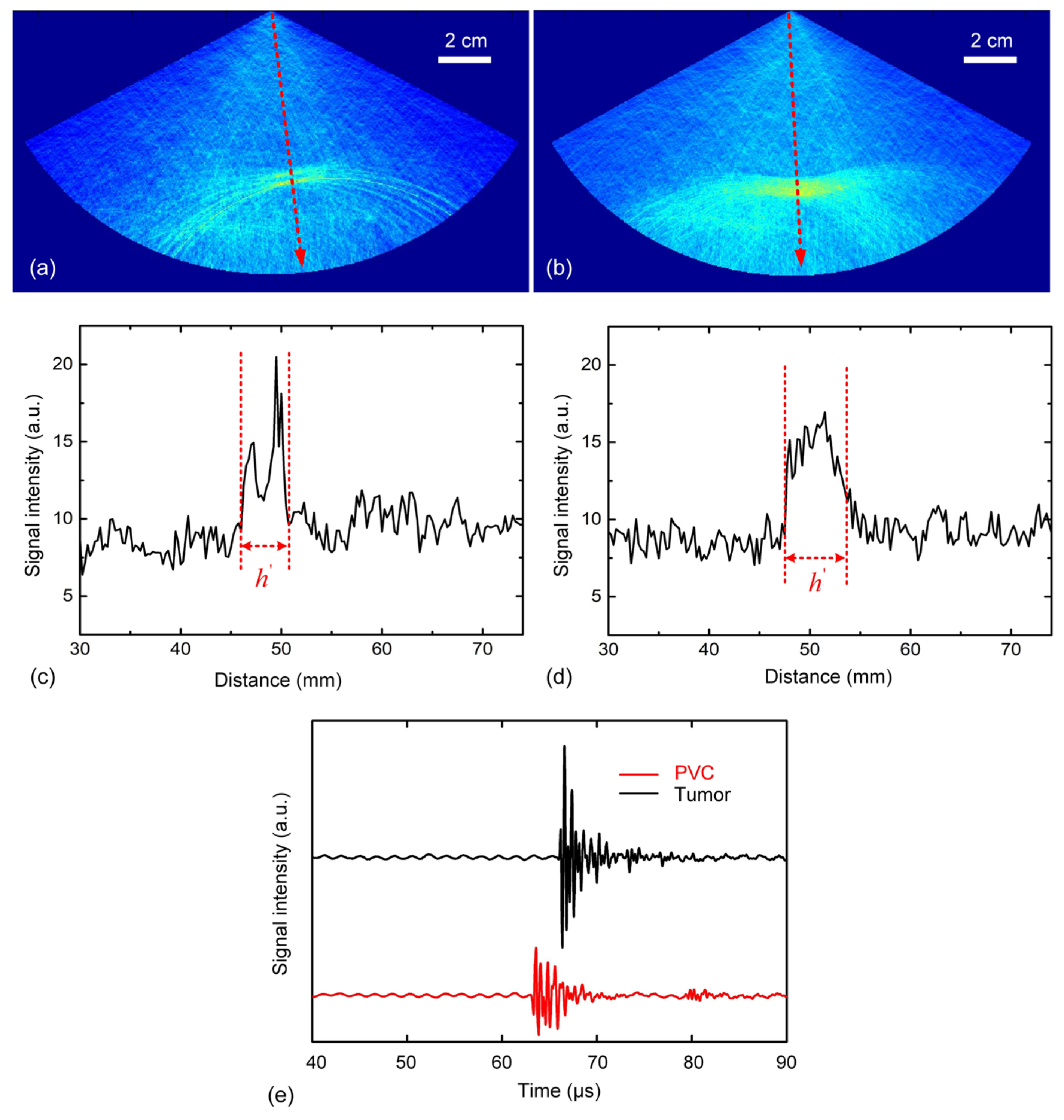
3.2. Two-Layer Situations

In some special cases, there is a large difference in the relative velocity of the material with respect to water, and the obvious acoustic impedance in the boundary can limit the reception of ultrasound from the point source, so the thickness of the MASO is difficult to obtain. By using 1/3 of a full ring transducer (1–128 elements) on the original signal to reconstruct images, we obtained the image in Figure 4b, which shows muscle tissue with the inclusion of glass material whose ultrasound propagation speed is considerably larger than that of water.

The thickness of the glass inclusion cannot be identified from the MTI image due to the incomplete boundary information of the image. The transmission time t from the trigger to the receiving point can be obtained from the time domain signal spectrum in Figure 4c. In this experiment, v_w is chosen to be 1500 m/s at room temperature, and l is fixed at 100 mm. The above results represent the identification of a type of MASO with an ultrasonic velocity considerably larger than that of water. For comparison, the reconstructed MTI image of muscle tissue without the inclusion is shown in Figure 4a and the corresponding time domain signal at t is shown in Figure 4c. As shown in Figure 4c, it can be seen that the ultrasonic signal emitted from the point sound source is received by the transducer after passing through the muscle tissue, and the signal peak appears at 65–67 μs on the time axis. This is very close to the transmission time of 66.7 μs at the same transmission distance in water, indicating that the difference in ultrasonic speed between the muscle sample being measured and water is very small.

In either case, the apparent thickness h′ can be obtained, and the ultrasound propagation speed through the MASO can be calculated according to Equation (3) when the acoustic impedance between them is not large enough to limit the reception of the ultrasonic signal. Usually, as with other biological soft tissues, the ultrasonic velocity though a tumor is similar to that of muscle tissue, while the ultrasonic velocity of polyvinyl chloride (PVC) is far less than that of muscle. In this case, the muscle tissue embedded with the tumor and the PVC is imaged by the US-MTI system, as shown in Figure 5a,b. The apparent thicknesses h′ of the tumor and the PVC are approximately 7.2 mm and 5.1 mm, respectively, which can be identified from the intensity profiles of the images in Figure 5c,d. The red vertical line is the 6dB threshold boundary [16]. The transmission times t are approximately 66.4 μs and 64.6 μs, respectively, as shown in Figure 5e. The propagation velocity through the MASO (v_s) can be calculated by substituting h′ and t into Equation (3), which is 1580 m/s in the case of the tumor and 2411 m/s in the PVC; the estimated values are broadly in line with the actual situation.

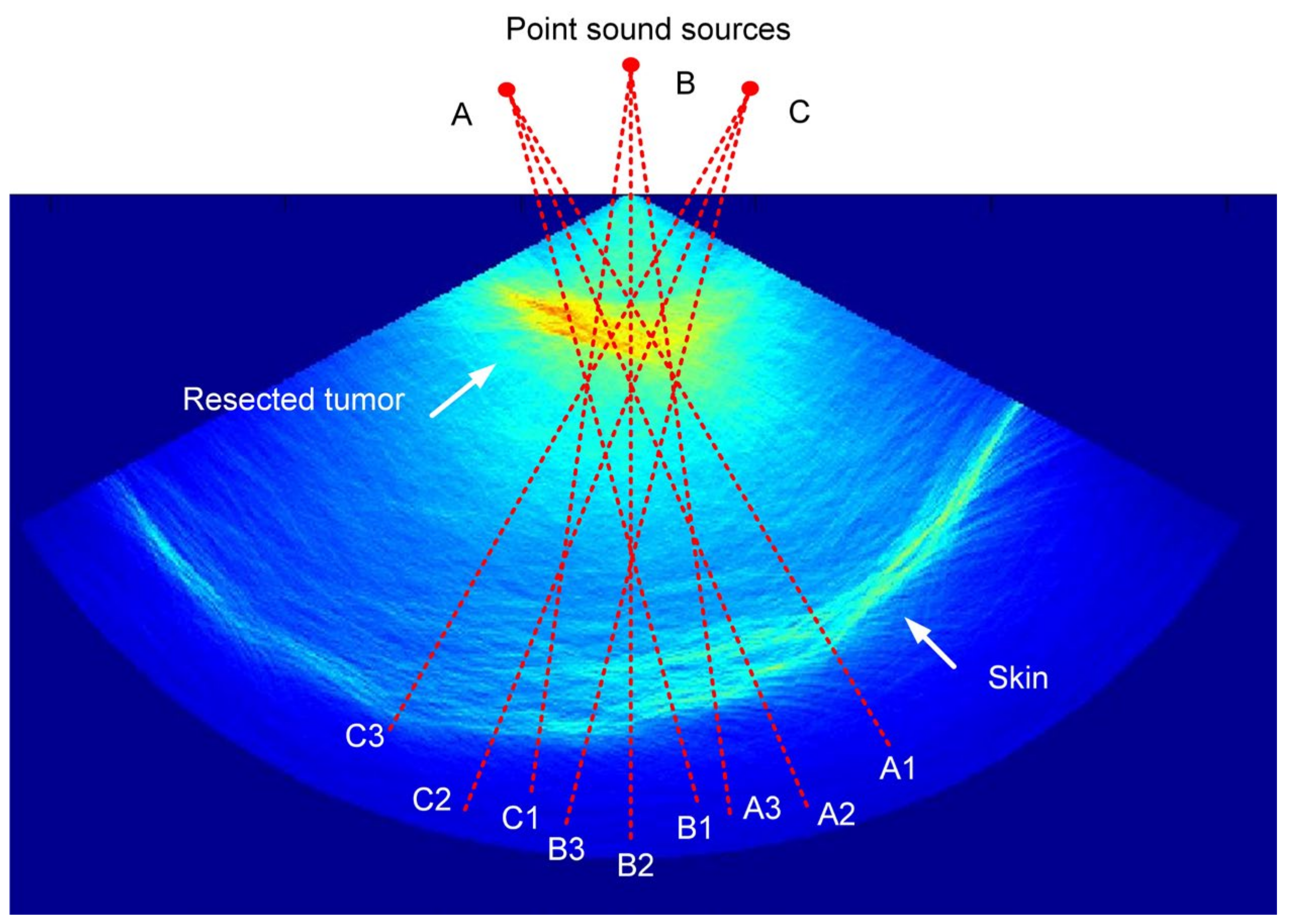
3.3. Three-Layer Situations

The above experiments were conducted in a case where there were two uniform layers. In order to make a more realistic experimental model, a three-layer situation should be considered. To this end, a resected tumor has been inserted into a resected breast from a sheep, which is used to simulate the detection of breast cancer. In this experiment, the velocity of ultrasound in both the coupled water and the sheep’s breast is known, and these values are about 1500 m/s and 1540 m/s, respectively. It should be noted that the skin is not considered due to the similarity of its ultrasonic velocity to that of the breast, and its low thickness. In this case, an ex vivo sheep breast embedded with a tumor is imaged by the US-MTI system, as shown in Figure 6.

The velocity of ultrasound in the tumor is obtained by numerical calculation, as shown in

Table 2. A list of parameters for the process of calculating.

	A1	A2	A3	B1	B2	B3	B1	B2	B3
$l$ (mm) Setted	150	150	150	150	150	150	150	150	150
$d$ (mm) Measured	98	92	114	100	89	94	102	89	117
$h^{\prime }$ (mm) Measured	8	12	9	10	15	13	14	10	12
$t$ (μs) Measured	100.6	98.1	99.7	99.2	96.2	97.5	96.7	99.5	97.7
$v_s$ (m/s) Calculated	1521	1511	1507	1522	1531	1551	1514	1523	1524
${\overline{v}}_s$ (m/s) Calculated	1522 (13)

l: transmission length; d: thicknesses of sheep breast; h′: thicknesses of tumor; t: transmission time; v_s: ultrasonic velocity of tumor; and SD: standard deviation.

. A1~A3, B1~B3, and C1~C3 represent different sound transmission paths in the experiment, which are marked by red lines in Figure 6. The transmission length l of all nine paths is set to 150 mm, and d and h′ represent the thicknesses of the sheep breast and tumor, which can be identified from the intensity profiles of the images in Figure 6, and are approximately 100 mm and 12 mm. The variable t is the transmission time calculated using the received ultrasonic signal, and is approximately 100 μs. The mean calculated value is 1522 m/s, which is close to 1520 m/s, which is the value calculated by substituting h′, d, and t into Equation (1) in the isolated tumor situation.

4. Discussion

The velocity of ultrasound is a function of the temperature. According to the ultrasonic manual, the velocity–temperature characteristic of water can be expressed by the following formula [28]:

$$\begin{array}{l}c=1402.336+5.03358T-5.79506\times {10}^{-2}{T}^2\\ +3.31636\times {10}^{-4}{T}^3-1.45262\times {10}^{-6}{T}^4+3.0449\times {10}^{-9}{T}^5\end{array}$$

(4)

where c is the velocity of ultrasound in water (m/s) and T is the temperature (°C) [28]. Assuming that the temperature of the human body ranges from 35 to 40 °C, the velocity of ultrasound can range from 1519.7 to 1528.8 m/s [28]. Thus, the error produced by temperature difference is less than 10 m/s, and can be ignored. Similar situations exist in other materials. In this paper, sample experiments were done at room temperature (26 °C), where the velocity of ultrasound in water was about 1499.2 m/s according to Equation (4). It is, therefore, reasonable to take 1500 m/s as the velocity of ultrasound in water. In order to obtain more accurate measurements, temperature measurement can be introduced in the future.

The parameters l and v_w can be accurately measured for the calculation of velocity using Equation (2); therefore, the accuracy of parameters t and h is vital in calculations of ultrasonic velocity. Generally speaking, the accuracy of t is mainly dependent on the frequency of the ultrasonic transducer and can be expressed as Δt~0.5/f = 0.05 μs. Another source of error in the estimation of t is the size of the ultrasound point source D [29,30,31], which can be expressed as Δt~0.1D/v = 0.034 μs, where v is velocity of ultrasound through the point source. Thus, the maximum theoretical error in the estimation of t for the US-MTI system is approximately 0.084 μs.

The implementation of the proposed method is based on two conditions; one is to receive the ultrasound from the point source with a signal-to-noise ratio of no less than 6 dB. The transmittal attenuation of ultrasound with a frequency of several MHz can be neglected in a homogeneous medium, but the reflections can weaken the received signal. When there is a larger acoustic impedance difference between the MASO and the normal tissue, such as in the cases of glass and metal, no ultrasonic signal will be received; therefore, the MASO can be considered as a foreign body with a high acoustic impedance difference, as in Figure 4b. Another condition is the existence of a time difference between the imaging area with and without the MASO. The time difference can be calculated from Equation (2):

$$\Delta t=h({\displaystyle \frac{1}{v_s}}-{\displaystyle \frac{1}{v_w}})$$

(5)

Therefore, the sensitivity of the measurement is highly dependent on the thickness and the ultrasonic velocity to be measured. Additionally, the measurement is more accurate with a thicker MASO. Considering the experimental US-MTI system as an example, the maximum error of t is approximately 0.084 μs and the ultrasonic velocity v_w is estimated as 1500 m/s. When the thickness h is 10 mm, the minimum detectable difference between v_s and v_w is approximately equal to 20 m/s for the worst estimate, and when h is 5 mm, that value will increase to about 40 m/s. Therefore, in future, the accuracy can be significantly improved by using a high-frequency transducer and a small sound point source. The resolution of MTI can reach hundreds of microns [15]. Thus, the smallest anomaly that can be detected in MTI can theoretically also reach hundreds of microns. On the other hand, the accuracy of ultrasonic velocity measurement decreases with the decreasing of size of the anomaly. In the present system, when the size of the anomaly is 5 mm, the inaccuracy will reach 40 m/s, which can be regarded as the maximum tolerable value. The existence of errors in the velocity measurement leads to an inability to exactly determine the materials with velocity differences within the error range. In future, using a high-frequency detector and a small ultrasound point source will improve the accuracy of detection, reducing the smallest measurable size of an anomaly to some extent.

The US-MTI system possesses the advantages of fast data acquisition and data processing. By using multiple-element transducers and a parallel DAS, the raw data can be acquired within about 20 ms for a two-dimensional image [12]. Additionally, as a result of the back-projection algorithm, without an iterative process, the data processing can be completed within about 5–10 ms. When multilayer (<30) data are needed, the whole processing time can be reduced to less than 1 s. The reduction of detection time is conducive to reducing the exposure time to microwaves, so patients can be physically and psychologically comfortable. Therefore, the proposed system can be used for regular systemic screening.

A key concern regarding the use of MTI for biological tissue is the radio frequency electromagnetic waves’ safety, based on the maximum permissible exposures (MPE) recommended by the Institute of Electrical and Electronics Engineers (IEEE) [32]. The MPE is dependent on pulse width, power density, repetition frequency, exposure duration, and the tissue type exposed. For exposures in controlled environments, the peak value of the mean squared field strength should not exceed the average power density (20 mW/cm²) at frequencies between 300 MHz and 6 GHz, according to the IEEE standard. With the present microwave source, the energy density of a single pulse is estimated to be about 15 to 360 μJ/cm² [16]. At 10 pulses per second, which is the most commonly used repeat frequency, the power density is about 0.15 to 3.6 mW/cm², which is less than the IEEE standard. For the microwave range, with frequencies between 300 MHz and 300 GHz, the photon energy is 1.24 × 10⁻⁶ eV to 1.24 × 10⁻³ eV, which is much less than the bond dissociation energy of protein, so the ionization effect in this case is extremely weak.

5. Conclusions

In this paper, a US-MTI system is presented that measures ultrasonic velocity as an additional parameter to determine the category of MASOs. The system allows for simultaneous MTI and ultrasonic velocity measurements within the same excitation and DAS, enhancing measurement accuracy while significantly reducing data acquisition and processing time. In our experiments, the system successfully demonstrated its ability to distinguish between exogenous anomalies (with ultrasound velocities markedly different from those of biological tissue) and endogenous anomalies (with ultrasound velocities similar to those of biological tissue). This enhanced MTI system, with its multi-parameter features, enables rapid diagnosis and identification of microwave-absorbing abnormal regions, greatly aiding diagnostic personnel in making informed decisions for further treatment planning.

References

1. Liu, Q.; Liang, X.; Qi, W.; Gong, Y.; Jiang, H.; Xi, L. Biomedical microwave-induced thermoacoustic imaging. J. Innov. Opt. Health Sci. 2022, 15, 2230007. [Google Scholar] [CrossRef]
2. Wang, B.; Sun, Y.; Wang, Z.; Wang, X. Three-Dimensional Microwave-Induced Thermoacoustic Imaging Based on Compressive Sensing Using an Analytically Constructed Dictionary. IEEE Trans. Microw. Theory Tech. 2020, 68, 377–386. [Google Scholar] [CrossRef]
3. Wu, L.; Cheng, Z.; Ma, Y.; Li, Y.; Ren, M.; Xing, D.; Qin, H. A Handheld Microwave Thermoacoustic Imaging System with an Impedance Matching Microwave-Sono Probe for Breast Tumor Screening. IEEE Trans. Med. Imaging 2022, 41, 1080–1086. [Google Scholar] [CrossRef] [PubMed]
4. Chi, Z.; Huang, L.; Wu, D.; Long, X.; Xu, X.; Jiang, H. First assessment of thermoacoustic tomography for in vivo detection of rheumatoid arthritis in the finger joints. Med. Phys. 2022, 49, 84–92. [Google Scholar] [CrossRef] [PubMed]
5. Singhvi, A.; Boyle, K.C.; Fallahpour, M.; Khuri-Yakub, B.T.; Arbabian, A. A Microwave-Induced Thermoacoustic Imaging System with Non-Contact Ultrasound Detection. IEEE Trans. Ultrason. Ferroelectr. Freq. Control 2019, 66, 1587–1599. [Google Scholar] [CrossRef]
6. Tamimi, E.A.; Xin, H.; Witte, R.S. Real-time 3D thermoacoustic imaging and thermometry using a self-calibration technique. Appl. Opt. 2020, 59, G255. [Google Scholar] [CrossRef] [PubMed]
7. Hu, Y.; Zhang, X.; Su, N.; Shi, X.; Chen, J.; Wu, H.; Liu, G.; Li, L.; Bai, C.; Xiu, J.; et al. Mechanical characterization of osteoporosis based on x-ray induced acoustic computed tomography. Appl. Phys. Lett. 2023, 123, 063701. [Google Scholar] [CrossRef]
8. Zhang, W.; Li, J.; Yang, S. Real-time interleaved photoacoustic and ultrasound imaging for guiding interventional procedures. Appl. Acoust. 2019, 156, 1–6. [Google Scholar] [CrossRef]
9. Huang, L.; Zheng, Z.; Chi, Z.; Jiang, H. Technical Note: Compact thermoacoustic imaging system based on a low-cost and miniaturized microwave generator for in vivo biomedical imaging. Med. Phys. 2021, 48, 4242–4248. [Google Scholar] [CrossRef]
10. Kruger, R.A.; Miller, K.D.; Reynolds, H.E.; Kiser, W.L.; Reinecke, D.R.; Kruger, G.A. Breast Cancer in Vivo: Contrast Enhancement with Thermoacoustic CT at 434 MHz—Feasibility Study. Radiology 2000, 216, 279–283. [Google Scholar] [CrossRef]
11. Ji, Z.; Lou, C.; Yang, S.; Xing, D. Three-dimensional thermoacoustic imaging for early breast cancer detection. Med. Phys. 2012, 39, 6738–6744. [Google Scholar] [CrossRef] [PubMed]
12. Ji, Z.; Ding, W.; Ye, F.; Lou, C. Handheld Thermoacoustic Scanning System Based on a Linear-array Transducer. Ultrason. Imaging 2016, 38, 276–284. [Google Scholar] [CrossRef] [PubMed]
13. Nie, L.; Xing, D.; Yang, D.; Zeng, L.; Zhou, Q. Detection of foreign body using fast thermoacoustic tomography with a multielement linear transducer array. Appl. Phys. Lett. 2007, 90, 174109. [Google Scholar] [CrossRef] [PubMed]
14. Nie, L.; Xing, D.; Yang, S. In vivo detection and imaging of low-density foreign body with microwave-induced thermoacoustic tomography: In vivo foreign body detection with thermoacoustic tomography. Med. Phys. 2009, 36, 3429–3437. [Google Scholar] [CrossRef] [PubMed]
15. Lou, C.; Yang, S.; Ji, Z.; Chen, Q.; Xing, D. Ultrashort Microwave-Induced Thermoacoustic Imaging: A Breakthrough in Excitation Efficiency and Spatial Resolution. Phys. Rev. Lett. 2012, 109, 218101. [Google Scholar] [CrossRef]
16. Ye, F.; Ji, Z.; Ding, W.; Lou, C.; Yang, S.; Xing, D. Ultrashort Microwave-Pumped Real-Time Thermoacoustic Breast Tumor Imaging System. IEEE Trans. Med. Imaging 2016, 35, 839–844. [Google Scholar] [CrossRef]
17. Kellnberger, S.; Hajiaboli, A.; Razansky, D.; Ntziachristos, V. Near-field thermoacoustic tomography of small animals. Phys. Med. Biol. 2011, 56, 3433–3444. [Google Scholar] [CrossRef]
18. Wu, X.; Luo, Z.; Wang, S.; Zhang, H. The researches on convolutional beamforming for linear-array photoacoustic tomography. Appl. Acoust. 2022, 186, 108441. [Google Scholar] [CrossRef]
19. Zhang, C.; Wang, Y. A reconstruction algorithm for thermoacoustic tomography with compensation for acoustic speed heterogeneity. Phys. Med. Biol. 2008, 53, 4971–4982. [Google Scholar] [CrossRef]
20. Stefanov, P.; Uhlmann, G. Thermoacoustic tomography with variable sound speed. Inverse Probl. 2009, 25, 075011. [Google Scholar] [CrossRef]
21. Agranovsky, M.; Kuchment, P. Uniqueness of reconstruction and an inversion procedure for thermoacoustic and photoacoustic tomography with variable sound speed. Inverse Probl. 2007, 23, 2089–2102. [Google Scholar] [CrossRef]
22. Jin, X.; Wang, L.V. Thermoacoustic tomography with correction for acoustic speed variations. Phys. Med. Biol. 2006, 51, 6437–6448. [Google Scholar] [CrossRef]
23. Li, C.; Duric, N.; Littrup, P.; Huang, L. In vivo Breast Sound-Speed Imaging with Ultrasound Tomography. Ultrasound Med. Biol. 2009, 35, 1615–1628. [Google Scholar] [CrossRef] [PubMed]
24. Mast, T.D. Empirical relationships between acoustic parameters in human soft tissues. Acoust. Res. Lett. Online 2000, 1, 37–42. [Google Scholar] [CrossRef]
25. Ophir, J.; Lin, T. A calibration-free method for measurement of sound speed in biological tissue samples. IEEE Trans. Ultrason. Ferroelectr. Freq. Control 1988, 35, 573–577. [Google Scholar] [CrossRef] [PubMed]
26. Anderson, M.E.; Trahey, G.E. The direct estimation of sound speed using pulse–echo ultrasound. J. Acoust. Soc. Am. 1998, 104, 3099–3106. [Google Scholar] [CrossRef] [PubMed]
27. Nebeker, J.; Nelson, T.R. Imaging of Sound Speed Using Reflection Ultrasound Tomography. J. Ultrasound Med. 2012, 31, 1389–1404. [Google Scholar] [CrossRef]
28. Ma, D.; Shen, H. Acoustic Manual; Science Press: Beijing, China, 2004; pp. 123–135. [Google Scholar]
29. Tserevelakis, G.J.; Zacharakis, G. High precision photoacoustic interferometer for the determination of the speed of sound in liquid media. Opt. Express 2022, 30, 28559–28568. [Google Scholar] [CrossRef]
30. Tserevelakis George, J.; Charalampos, A.; Giannis, Z. Optoacoustic interferometric characterization system (OPTICS) for the evaluation of fuel quality through speed of sound measurements. Ultrasonics 2024, 139, 107291. [Google Scholar] [CrossRef]
31. Kolkman, R.G.M.; Steenbergen, W.; van Leeuwen, T.G. Reflection mode photoacoustic measurement of speed of sound. Opt. Express 2007, 15, 3291–3300. [Google Scholar] [CrossRef]
32. C95.1 2005; IEEE Standard for Safety Levels with Respect to Human Exposure to Radio Frequency Electromagnetic Fields 3 kHz to 300 GHz. IEEE: New York, NY, USA, 2005.
Figure 1. The model of the measurement of ultrasonic velocity.
Photonics 11 00916 g001
Figure 2. (a) A photograph of the detection section. (b) A diagram of the whole experimental setup.
Photonics 11 00916 g002
Figure 3. (a) The transmission time along with the sample thickness, h, of two kinds of materials—Polyfoam (Pol) and Polymethyl methacrylate (PoM). The velocity of ultrasound in Polyfoam (vs) is less than that of water (vw), and the velocity of ultrasound in Polymethyl methacrylate (vs) is larger than that of water (vw), so the Pol curve is rising, and the PoM is falling. (b,c) The reconstructed MTI images of the sample (a rubber) with/without ultrasonic velocity difference (5% Agar). The inset images are the X-ray images of the sample. The error bars were added based on the triplicate samples and our measurements.
Photonics 11 00916 g003
Figure 4. (a) The reconstructed MTI images of muscle tissue (a) without and (b) with glass inserted are displayed. (c) The MTI signal is generated by the point absorber in the geometric center, and transmitted along the two red lines of (a) and (b), respectively. (NA: not available, without the glass inserted).
Photonics 11 00916 g004
Figure 5. (a) The MTI image of muscle tissue with a PVC insertion. (b) The MTI image of muscle tissue with a tumor. (c,d) The intensity profiles extracted from (a,b) along two red lines passing through the sample center. The apparent thicknesses of the MASOs in the MTI images have been marked. (e) The MTI signal generated by the point absorber in the geometric center transmitting along the two red lines of (a) and (b), respectively.
Photonics 11 00916 g005
Figure 6. The MTI image of a sheep breast embedded with a tumor. The nine paths marked by red lines represent the different sound transmission paths in the experiment. A1–C3: the sound transmission paths.
Photonics 11 00916 g006