Abstract
The distribution of diffuse spot energy can be used to sensitively evaluate the aberrations and defects of optical systems. Therefore, the objective and quantitative measurement of diffuse spot parameters is an important means to control the detection quality of space debris detection systems. At present, the existing optical system dispersion measurement method can only judge whether the energy distribution meets the index. However, these methods ca not provide an objective quantitative basis to guide the installation process. To solve this problem, a mathematical simulation model of 3D multi-phase sub-pixel PSF distribution is proposed. According to the relation between the CCD target plane and the theoretical image plane (focal plane, defocus, and deflection), the diffuse spot distribution of the optical system is simulated with different phase combinations. Then, Pearson Correlation Coefficient (PCC) is used to evaluate the matching similarity of the diffuse spot image. The simulation results show that when the PCC is greater than 0.96, the distribution of the two diffuse spots can be identified as matching. This also confirms the accuracy of the proposed PSF model. Then, the focusing deviation of the system being tested can be analyzed according to the phase size of the diffuse spot simulation image. This method can quickly and accurately guide the focal surface installation and testing of the system. Therefore, the purpose of improving the detection accuracy of space debris is achieved. It also provides a quantitative basis for the engineering application of optical detection systems in the future.
1. Introduction
With the increasing frequency of space launch activities, the amount of space debris increases rapidly. It makes orbital resources become very scarce and seriously threatens the safety of spacecraft in orbit [1,2]. Therefore, in order to develop and utilize space resources safely and continuously, it is necessary to continuously improve the tracking and monitoring technology of space debris, enhance the detection and identification ability of space debris, and master the target characteristics and distribution dynamics of space debris [3].
Optical observation is an important means of space debris monitoring, and the detection performance of optical systems is crucial to the quality of space debris research. For some detection optical systems such as telescopes (ground-based and space-based), it is necessary to acquire the model of the PSF. The PSF model is one of the important technical indexes to evaluate the detection optical system. If the PSF model is built accurately, the accurate star point diffuse spot distribution can be simulated accurately [4,5,6].
At present, there are probably two mainstream methods for PSF modeling estimation. One is the parametric method. Physical parameters of the detection system can be used to build a PSF model, such as the relative aperture, focal length, wavelength, and other parameters. Firstly, the estimation precision is set according to the task requirement, and then the model complexity is determined. Generally, the higher the accuracy requirement of the PSF, the higher the complexity of the model will be. The PSF model is used to simulate the star target image. The second method is not to use the parameter model. The star point target at different positions of the field of view is used as the measurement value of the PSF across the field of view, and the PSF of the star point or other positions is estimated based on the data.
In 1969, Moffat proposed the classic Moffat PSF model [7]. The PSF model is represented by a function of N empirical parameters, where N is not fixed. Usually, the Moffat model is accurate with only two parameters. Moffat distribution can accurately describe the point spread function in star point simulation, but neither Gaussian distribution nor Lorentz distribution can accurately describe the characteristics of the point spread function in both wings. Generally, the PSF appears as a sharp correction peak and a wide halo extension, and the Moffat model is still widely used today because of its good approximation to the PSF peak. Simon Zieleniewski proposed a PSF modeling method using fine parameters, which interpolates PSFs of different wavelengths [8,9], as shown in Figure 1. This model method can use harmonics to create accurate and computationally efficient PSF data cubes. The PSF varies significantly with the wavelength and type of AO system, so it is necessary to create a detailed PSF in all wavelength channels for accurate simulation. The AO simulations showed that a single PSF introduced misleading features into the simulated observations of HARMONI, so an analytical model was used to parameterize the PSF as a function of the wavelength for interpolation. Serre et al. show that the PSF of the VLT telescope MUSE can be accurately modeled from the Moffat profile, where two parameters vary smoothly with wavelength. Using the point extension function fitting code eltPSFfit developed by J. Liske, Simon Zieleniewski et al. could fit the radial profile of each PSF using several analytic functions. Domestic Mingying et al. carried out modeling of the PSF using the Cauchy distribution [10].
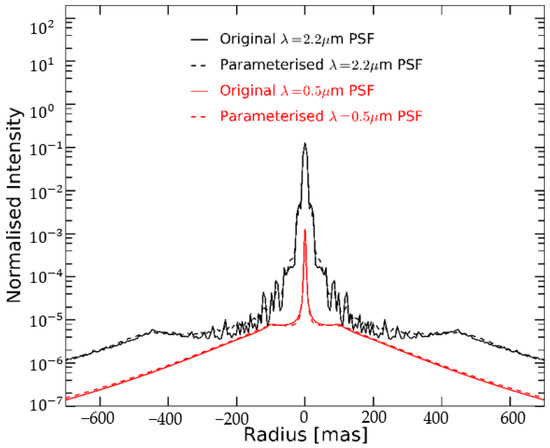
Figure 1.
Radial profiles of original and parameterized PSFs at λ = 0.5 µm and λ = 2.2 µm.
As we know, the modeling methods of the PSF both at home and abroad are mainly based on parameter modeling. The substantial advantage of the parametric PSF is to compress all the important information about the physical PSF into a small number of parameters. The values of these parameters can be used for comparison, correlation, or any statistical analysis. In the aspect of data-driven non-parametric PSF modeling, a large amount of test data is needed as a reference for estimation. However, there are often errors in the test data, and the resulting estimates are not very accurate.
The multi-phase sub-pixel PSF simulation analysis method proposed in this paper not only uses the parameters of the optical system, but also comprehensively considers the phase distribution characteristics of the point source array. Based on different phase point sources, sub-pixel sampling is performed to realize sub-pixel PSF reconstruction. The simulated diffuse spot distribution is more accurate using this proposed method. Through comparison and analysis with the actual star distribution map, it can provide more accurate and reliable interpretation data for focusing work.
Therefore, according to the optical dispersion theory, this paper theoretically analyzes the possible relationship between the focal plane and the theoretical image plane of the CCD and proposes a 3D multi-phase sub-pixel PSF estimation method. This proposed method is not only using the parameters of the optical system, but the phase distribution characteristics of the point source array are also considered comprehensively. Based on the results of the comparison between two traditional algorithms and the proposed algorithm, the advantages of the 3D multi-phase sub-pixel PSF estimation method are obvious. In addition, this paper also proposes a comparison of the energy distribution of the dispersion spot simulation image with the actual image. Then, the energy distribution deviation of the star spot image is given quantitatively. Compared with the traditional focusing method, the subjective factors are eliminated, the inspection standard is unified, and the quantitative basis is provided for the focal plane adjustment and testing of the optical system.
2. Multi-Phase Sub-Pixel PSF Estimation
2.1. Principle of Star Detection
According to the Fraunhofer diffraction theory, the light intensity distribution of the diffraction image is no longer an ideal image point but a diffuse spot after passing through the optical system. That is called the Point Spread Function (PSF). In the ideal star point imaging, the light intensity before and after the image plane is symmetrically distributed and changes with the different field of view. However, in the actual optical system imaging, aberration can easily destroy this symmetry. The dispersion energy distribution can reflect the optical aberrations and defects very sensitively, so the imaging quality of the optical system can be controlled via quantitative measurement of the dispersion parameters [11,12].
The intensity distribution of the point source depends on the shape of the pupil. For an ideal optical system, the intensity distribution of the star image only depends on the pupil shape [13]. In the case of a circular pupil, the light intensity distribution of the star image in the focal plane is the airy spot’s light intensity distribution. The energy formula of the diffuse spot is defined as follows:
where I/I0 is the relative intensity (the center of the star diffraction image is defined as 1.0), is the first-order Bessel function, is the relative aperture, and is the radial distance away from the center of the star diffraction image. The physical significance of the above parameters is shown in Figure 2 [14,15]. The airy spot consists of a central bright spot and a few concentric outer rings with rapidly diminishing brightness [16].
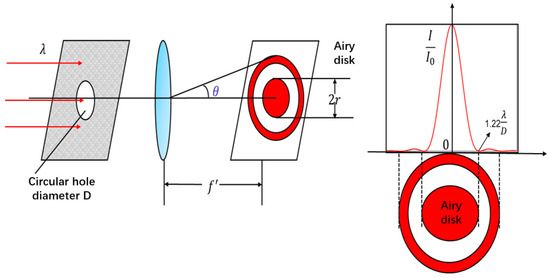
Figure 2.
Diffraction limited parameters and intensity distribution of airy spot.
The expression for the proportion of energy falling in the circle is expressed as follows [17]:
where is the 0 order Bessel function, and is the 1 order Bessel function.
2.2. Focal Plane Distribution of Optical System
According to the light intensity distribution of the image plane and the characteristics of the optical path, the relationship between the CCD target plane and the theoretical image plane can be divided into three types, namely the focal plane, defocus, and deflection, as shown in Figure 3.
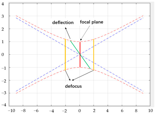
Figure 3.
Relationship between the CCD target plane and the theoretical image plane.
The expression of the three-dimensional distribution function of the two-dimensional diffuse spot is shown as follows [18]:
When defocus occurs, there is a ratio of amplification ( > 1), and the equations are and . Then, the diffuse spot distribution function can be obtained as . When deflection occurs, the equation is . We use linear approximation at the deflection, is , and is . The distribution function of the diffuse spot is expressed as. The distribution of the three types is clearly shown in Figure 4.
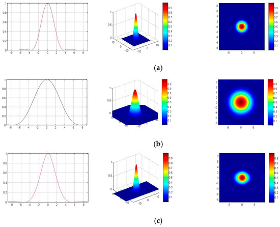
Figure 4.
Energy distributions of focal plane, defocus, and deflection. (a) focal plane. (b) defocus. (c) deflection.
2.3. Simulation Analysis of Standard Diffuse Spot Distribution
For conventional detection systems, the energy concentration of the optical system is generally required to account for 80% in 2 × 2 pixels. Combined with the design technical index, the radius of an 80% energy spot is equal to the pixel size of the detector. For ease of calculation and description, the size of 2 × 2 pixels is the largest external square of the 80% energy spot. Although the response area of 2 × 2 is 27.3% and is larger than the 80% energy patch, this does not add much energy as seen from the energy percentage curve [19]. Therefore, it is reasonable to use the pixel whose size is equal to 80% of the radius of the energy spot.
In the simulation process, the phase of the star target source in the image represents its normalized position in one pixel, and the phase value interval is from 0 to 1. When the phase is 0, it means that the point source falls into one pixel exactly [20]. According to the theoretical definition of the PSF, this situation satisfies the direct sampling condition. As shown in Figure 5, the phase of the point source in the pixel (,) is and in the and directions, respectively. The gray level of the star target source is set as , and and represent the position of pixels in the image. Then, the gray level , , , and of the four pixels under phase action are, respectively, described as follows:
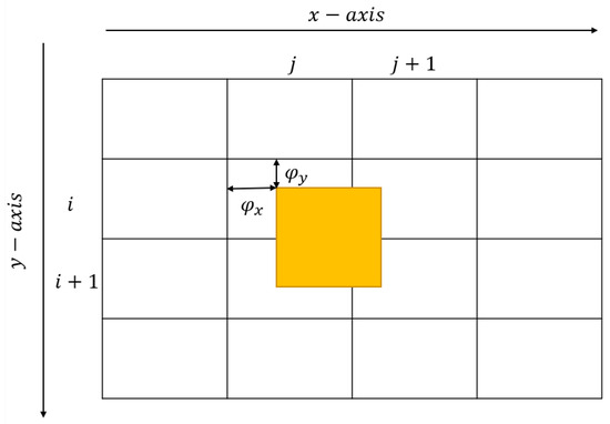
Figure 5.
Phase of star point.
In the simulation conditions of this paper, three types of relations between the CCD target plane and the theoretical image plane are simulated. And the three types are the focal plane, defocus, and deflection [21]. In addition, for each relation, it is also necessary to consider the sub-pixel PSF estimation of different phase point sources.
For a point target source in the surface source array, a window with a size of 5 × 5 pixels is extracted. And the normalized pixel position of the point source is defined as (, ). The local coordinate system is . The center of the window is the origin. and are parallel to the x and y directions, respectively, and the coordinates of and take the values of +2, +1, 0, −1, −2, respectively. Each pixel in the window is represented by two horizontal coordinate values (, ) in the PSF reconstruction coordinate system as follows [22]:
According to the target design geometry calculation, each phase (, ) of the window is determined. Here, take 1/8 pixel accuracy as an example in Figure 6. Each source point target moves to the adjacent point source in a phase of 1/8, such as an interval sequence of 0, 0.125, 0.25, 0.375, and 0.5. And the amplitude corresponding to the arrow represents the sampling value of each pixel. Similarly, 2D PSF reconstruction means that the phase moves in both x and y directions at the same time [23,24,25,26,27].
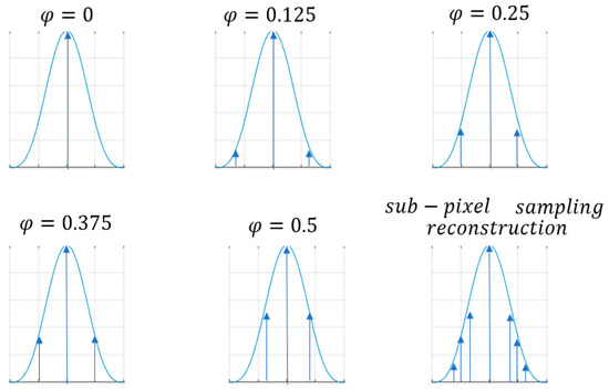
Figure 6.
One-dimensional PSF reconstruction via multi-phase.
According to the above principles, 3D (-dimension, -dimension, and gray-dimension) multi-phase sub-pixel PSF distribution simulation is carried out by focusing on the three states of focal plane, defocusing, and deflection, respectively [28,29]. Fifteen different sizes of phase shifts are given here, including 0 × 0, 0.125 × 0, 0.25 × 0, 0.375 × 0, 0.5 × 0, 0.125 × 0.125, 0.25 × 0.125, 0.375 × 0.125, 0.5 × 0.125, 0.375 × 0.25, 0.375 × 0.375, 0.5 × 0.5, 0.25 × 0.25, 0.5 × 0.25, and 0.5 × 0.375. The simulated energy distribution in the focal plane state is shown in Figure 7. The simulated energy distribution in the defocusing state is shown in Figure 8. The simulated energy distribution in the deflection state is shown in Figure 9.
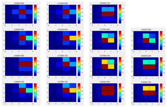
Figure 7.
The simulated energy distribution in the focal plane state.
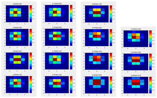
Figure 8.
The simulated energy distribution in the defocusing state.
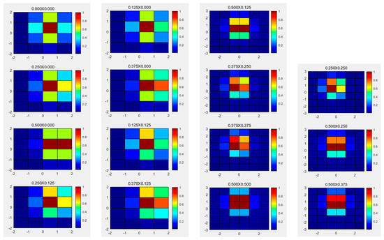
Figure 9.
The simulated energy distribution in the deflection state.
3. Collecting Images of the Diffuse Spot Distribution of the Actual Detection System
The actual diffuse spot measuring device of the optical system in this paper is mainly composed of a monochromator light source, optical bench collimator, high-precision turntable, detection system, and image acquisition system, as depicted in Figure 10. The star point is placed on the focal plane of the parallel optical tube and illuminated with a monochromator to form a target at infinite distance. The detection system is fixed on the turntable so that it is coaxial with the parallel optical tube. The turntable is turned during measurement and the image acquisition system is used to collect star point images [30,31]. In this way, the diffuse spot distribution data in different fields of view are obtained. Experimental data can be used as a database for subsequent comparative analysis with simulation images, as seen in Figure 11.
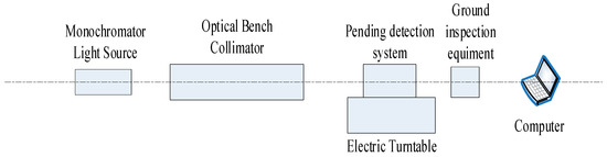
Figure 10.
Detection system diffuse spot measuring device.
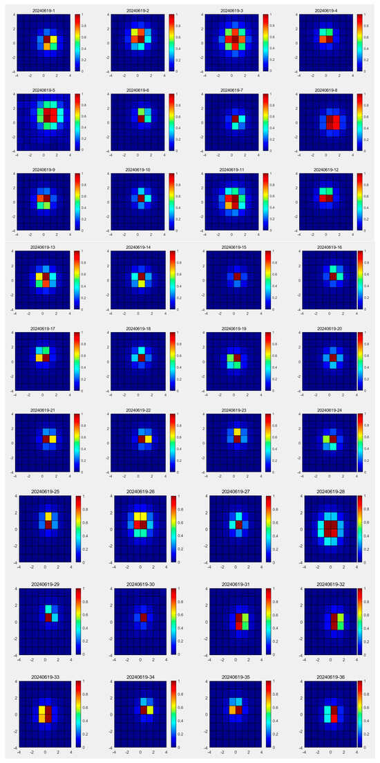
Figure 11.
The distribution of diffuse spots in the actual detection system.
From the distribution of various star diffuse spots as shown in Figure 10, the actual energy distribution of the space debris detection system is relatively complex and diverse. Only through subjective interpretation of the image can we reach the conclusion of defocusing. But it is impossible to clarify the technical direction of focusing. Therefore, we need to compare the dispersion spot distribution of the actual system with the above simulated diffuse spot distribution data template library one by one and objectively give the quantitative basis for focusing. Finally, this optical system quickly meets the target requirements.
4. Comparative Analysis of Standard Diffuse Spot Simulation Images and Actual Detection System Diffuse Spot Images
In order to evaluate the correlation and similarity between simulated dispersion images and the actual dispersion images, the PCC is used here [32,33]. The PCC is an evaluation index that measures the strength of the linear relationship between two continuous variables. The value of the PCC is between −1 and 1. It is expressed by the quotient of their respective covariance and variance.
Assuming that the simulated image and the measured image of the diffuse spot are and , respectively, the expression of covariance is described as follows:
The expression for the variance is defined as follows:
PCC is calculated and derived as follows:
Based on the above equations, the PCCs between the simulated images and the actual detection system diffuse spot images can be calculated. The simulated image with higher similarity to the actual diffuse spot image can be selected by comparison, so as to obtain the quantitative basis of focal plane adjustment. Figure 12 shows the distribution of the five groups of diffuse spot images using three PSF modeling methods. Column 1 contains the diffuse spot images obtained with the actual detection system. Column 2 contains the simulation images using the proposed 3D multi-phase sub-pixel PSF model. Column 3 contains the simulation images using Simon Zieleniewski’s method. Column 4 contains the simulation images using the classic Moffat PSF model.
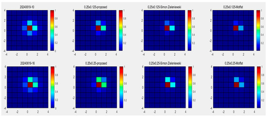
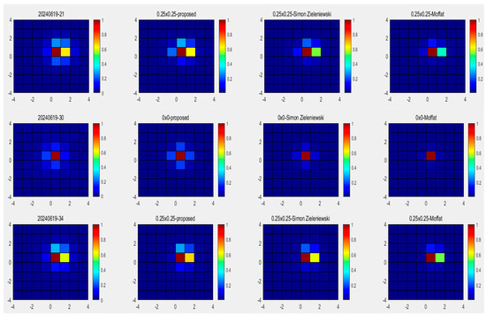
Figure 12.
Comparison of energy distribution between simulated diffuse spot simulation images and the actual detection system’s diffuse spot images.
Table 1 shows the PCCs among the five groups of matched images using these three methods. PCC-P represents the PCCs between the actual detection system’s diffuse spot images and images obtained with the proposed method.. PCC-S represents the PCCs between the actual detection system’s diffuse spot images and images obtained with Simon Zieleniewski’s method. PCC-M represents the PCCs between the actual detection system’s diffuse spot images and images obtained with the Moffat PSF model. In Table 1, it can be seen that the star distribution map obtained with the algorithm proposed in this paper is the closest to the actual image. When the PCC of the diffuse spot distribution of the two images is greater than 0.96, it can be concluded that these two diffuse spot distributions are similar.

Table 1.
Calculation of PCCs.
On one hand, the accuracy of the 3D multi-phase sub-pixel PSF estimation model used in this paper is verified. On the other hand, the simulation parameters of the simulated images provide reference information for the focal plane adjustment of the actual system. Through this method, the energy distribution of the detection system can be judged quickly and effectively, and the image quality of the optical system can be analyzed comprehensively, so as to meet the testing requirements of the optical system image quality in engineering projects.
5. Discussion
The 3D multi-phase sub-pixel PSF simulation analysis method proposed in this paper not only uses the parameters of the optical system, but also comprehensively considers the phase distribution characteristics of the point source array. This method performs sub-pixel sampling based on different phase point sources to realize sub-pixel PSF reconstruction. By using this method, the dispersion spot distribution can be simulated accurately, and the real situation of different phase movement can be simulated, too. Moreover, the data template library of the diffuse spot distribution is enriched. By comparison and analysis with the actual star distribution map, more accurate and reliable interpretation data can be provided for focusing work. Compared with the traditional focusing method, the method eliminates the subjective factors, unifies the inspection standard, and provides a quantitative basis for the focal plane adjustment and testing of optical system.
6. Conclusions
Aiming at the drawbacks of measuring the diffuse spot parameters of a space debris detection system, this paper proposes a mathematical model based on 3D multi-phase sub-pixel PSF estimation. The dispersion energy distribution of a space debris detection system is simulated using a 1/8 mobile phase. Then, based on the PCCs, the energy distribution of the standard diffuse spot simulation images is compared with those of the actual detection system. The deviation of the energy distribution of the star spot image is given quantitatively, the subjective factors are eliminated, and the testing criteria are unified. Therefore, the diffuse spot energy distribution of the optical system can be judged and analyzed quickly and accurately. It provides a quantitative basis for the installation and testing of the optical system. The method presented in this paper has important reference value in engineering testing.
Author Contributions
Conceptualization, F.B. and D.Y.; methodology, F.B. and D.Y.; data curation, F.B. and D.Y.; writing—original draft preparation, F.B.; writing—review and editing, F.B.; funding acquisition, D.Y. and Y.W. All authors have read and agreed to the published version of the manuscript.
Funding
This research was funded by the National Science and Technology Major Project (2022ZD0117301).
Institutional Review Board Statement
Not applicable.
Informed Consent Statement
Not applicable.
Data Availability Statement
All data are available from the authors upon reasonable request.
Conflicts of Interest
The authors declare no conflicts of interest.
References
- Liu, M.; Wang, H.; Yang, S.; Du, Y.; Wen, D.; Xue, Y. Space debris positioning technology based on observation by multiple optical platforms. In Proceedings of the AOPC 2019: Space Optics, Telescopes, and Instrumentation, Beijing, China, 7–9 July 2019; SPIE: Bellingham, WA, USA, 2019; Volume 11341. [Google Scholar]
- Hardy, T.J.; Cain, S.C. Characterizing Point Spread Function (PSF) fluctuations to improve Resident Space Object detection (RSO). In Proceedings of the Sensors and Systems for Space Applications VIII, Baltimore, MD, USA, 20–21 April 2015; SPIE: Bellingham, WA, USA, 2015; Volume 9469. [Google Scholar]
- Delaite, T.; Couetdic, J.; Glemet, E.; Cassaing, F. Performance of an Optical COTS Station for the wide-field Detection of Resident Space Objects. In Proceedings of the Advanced Maui Optical and Space Surveillance Technologies Conference (AMOS), Maui, HI, USA, 19–22 September 2023. [Google Scholar]
- Qi, L.; Sun, L.-C.; Gong, Z.-Z.; Rui, X.-B.; Zhang, P.-L.; Cui, Y.-H.; Zeng, J. Micro Space Debris Detection Technology and Applications. Space Debris Res. 2021, 21, 10–16. [Google Scholar]
- Vishnu Bharadwaj, B.G.; Samaga, V.V.K.; Navya, T.; Srinidhi, B.S.; Chandars, T.S. Active space debris detection, capture, and storage system. In Proceedings of the Asia Conference on Electronic Technology (ACET 2024), Singapore, 8–10 March 2024; SPIE: Bellingham, WA, USA, 2024; Volume 13211. [Google Scholar]
- Zhong, H.; Zhang, J.; Liang, S.; Wang, L. Space-Based Technology of Long-Range Wide-Field-of-View Detection, Identification and Tracking for Space Debris. Space Debris Res. 2019, 19, 1–12. [Google Scholar]
- Bendinelli, O.; Parmeggiani, G.; Zavatti, F. CCD Star Images: On the Determination of Moffat’s PSF Shape Parameters. J. Astrophys. Astron. 1988, 9, 17–24. [Google Scholar] [CrossRef][Green Version]
- Wu, X. Nonparametric Point Spread Function Model Based on Deep Neural Networks for Optical Telescopes. Master’s Thesis, Taiyuan University of Technology, Taiyuan, China, 2021. [Google Scholar]
- Zieleniewski, S.; Thatte, N. Parameterizing E-ELT AO PSFs for detailed science simulations for HARMONI. In Proceedings of the 3rd AO4ELT Conference, Florence, Italy, 26–31 May 2013. [Google Scholar]
- Liske, J. Database of Technical Data. Available online: http://www.eso.org/sci/facilities/eelt/science/drm/tech_data/ao/psf_fitting/ (accessed on 27 July 2013).
- Wang, F.; Chang, J.; Hao, Y.; Du, X.; Niu, Y. The point spread function modeling of the ultra-high accurate star tracker. Opt. Tech. 2016, 42, 24–27. [Google Scholar]
- Chen, L.; Rao, P.; Sun, Y.; Ren, Q.; Zhu, H. On Orbit Modulation Transfer Function Measurement Method of Space Camera Based on Star Points. Laser Optoelectron. Prog. 2020, 57, 161102. [Google Scholar] [CrossRef]
- Attarwala, A.A.; Hardiansyah, D.; Romano, C.; Roscher, M.; Molina-Duran, F.; Wangler, B.; Glatting, G. A Method for Point Spread Function Estimation for Accurate Quantitative Imaging. IEEE Trans. Nucl. Sci. 2018, 65, 961–969. [Google Scholar] [CrossRef]
- Yang, J.; Jiang, B.; Ma, J.; Sun, Y.; Di, M. Accurate Point Spread Function (PSF) Estimation for Coded Aperture Cameras. In Proceedings of the Optoelectronic Imaging and Multimedia Technology III, Beijing, China, 9–11 October 2014; Volume 9273. [Google Scholar]
- Beltramo-Martin, O.; Ragland, S.; Fétick, R.; Correia, C.; Dupuy, T.; Fiorentino, G.; Fusco, T.; Jolissaint, L.; Kamann, S.; Marasco, A.; et al. Review of PSF reconstruction methods and application to post-processing. In Proceedings of the Adaptive Optics Systems VII, Online, 14–18 December 2020; SPIE: Bellingham, WA, USA, 2020; Volume 11448. [Google Scholar]
- Fan, K. Research on Ground Measurement Method of PSF Ellipticity of Space Sky Survey Telescope; Changchun Institute of Optics, Fine Mechanics and Physics, University of Chinese Academy of Sciences: Beijing, China, 2021. [Google Scholar]
- Rundquist, N.E.; Wright, S.A.; Schöck, M.; Surya, A.; Lu, J.; Turri, P.; Chapin, E.L.; Chrisholm, E.; Do, T.; Dunn, J.; et al. The InfraRed Imaging Spectrograph (IRIS) for TMT: Photometric characterization of anisoplanatic PSFs and testing of PSF-Reconstruction via AIROPA. In Proceedings of the Ground-based and Airborne Instrumentation for Astronomy VIII, Online, 14–22 December 2020; SPIE: Bellingham, WA, USA, 2020; Volume 11447. [Google Scholar]
- Yang, T.; Zhou, F.; Xing, M. A Method for Calculating the Energy Concentration Degree of Point Target Detection System. Spacecr. Recovery Remote Sens. 2017, 38, 41–47. [Google Scholar]
- Akhmedov, D.; Yelubayev, S.; Ten, V.; Bopeyev, T.; Alipbayev, K.; Sukhenko, A. Software and mathematical support of Kazakhstani star tracker. In Proceedings of the Sensors, Systems, and Next-Generation Satellites XX, Edinburgh, UK, 26–29 September 2016; SPIE: Bellingham, WA, USA, 2016; Volume 10000. [Google Scholar]
- Gao, H.; Liu, W.; He, H. Static PSF Measurement Method of Satellite Borne Area CMOS Camera with Point Array. Spacecr. Recovery Remote Sens. 2017, 38, 53–60. [Google Scholar]
- Swindells, I.; Wheeler, R.; Darby, S.; Bowring, S.; Burt, D.; Bell, R.; Duvet, L.; Walton, D.; Cole, R. MTF and PSF Measurements of the CCD273-84 Detector for the Euclid Visible Channel. In Proceedings of the SPIE, Space Telescopes and Instrumentation 2014: Optical, Inreared, and Millimeter Wave, Montréal, QC, Canada, 28 August 2014; Volume 9143, p. 91432V. [Google Scholar] [CrossRef]
- Martin, S.R.; Flinois, T.L.B. Simultaneous sensing of telescope pointing and starshade position. J. Astron. -Instrum. Syst. 2022, 8, 014010. [Google Scholar] [CrossRef]
- Zeng, C.; Gao, K.; Zhang, Y.; Chen, X.; Xiao, Y. Centroid location of star sub-pixels based on iterative Lagrange interpolation. In Proceedings of the AOPC 2022: Optical Sensing, Imaging, and Display Technology, Beijing, China, 23 January 2023; SPIE: Bellingham, WA, USA, 2023; Volume 12557. [Google Scholar]
- Fufu, L.; Xu, W.; Liang, Z. Measurement Method of Random Errors in Spot Target Detection by Flat-Panel Detector. Acta Opt. Sin. 2021, 41, 0404001. [Google Scholar] [CrossRef]
- Lin, L.; Meng, Q.; Chen, J. A calculation method of operation range of infrared point target in photoelectric detection system based on considering the target diffuse spot. Optoelectron. Adv. Mater. Rapid Commun. 2023, 17, 286–294. [Google Scholar]
- Yueyong, L.; Chao, Z.; Zongte, X. Accuracy Analysis for Sub-Pixel Location of Star Image. J. Geomat. Sci. Technol. 2015, 32, 578–582. [Google Scholar]
- Brauers, J.; Seiler, C.; Aach, T. Direct PSF Estimation Using a Random Noise Target. In Proceedings of the Digital Photography VI, San Jose, CA, USA, 18 January 2010; Imai, F., Sampat, N., Xiao, F., Eds.; SPIE: Bellingham, WA, USA, 2010; Volume 7573. [Google Scholar]
- Wilson, T.M.; Xiong, X. Characterization of the VIIRS DNB mid-gain stage using observations of bright stars. In Proceedings of the Sensors, Systems, and Next-Generation Satellites XXVII, Amsterdam, The Netherlands, 3–7 September 2023; SPIE: Bellingham, WA, USA, 2023; Volume 12729. [Google Scholar]
- McVittie, G.R.; Enright, J. Color star tracking I: Star measurement. Opt. Eng. 2012, 51, 084402. [Google Scholar] [CrossRef]
- Zheng, R.; Liu, B.; Gao, Y.; Wang, L.; Chen, Q. Research on star points position analysis and simulation technology of infrared star simulators. Chin. J. Sci. Instrum. 2022, 43, 115–121. [Google Scholar]
- Zhang, P. Analysis of optimum time granularity selection in traffic prediction based on Pearson correlation coefficient. In Proceedings of the International Conference on Statistics, Data Science, and Computational Intelligence (CSDSCI 2022), Qingdao, China, 19–21 August 2022; SPIE: Bellingham, WA, USA, 2023; Volume 12510. [Google Scholar]
- Kirešová, S.; Rusyn, V.; Guzan, M.; Vorobets, G.; Sobota, B.; Vorobets, O. Utilizing low-cost optical sensor for the measurement of particulate matter and calculating Pearson’s correlation coefficient. In Proceedings of the Sixteenth International Conference on Correlation Optics, Chernivtsi, Ukraine, 18–21 September 2023; SPIE: Bellingham, WA, USA, 2024; Volume 12938. [Google Scholar]
- Ma, J.; Cuan, Y. Research on Pearson correlation and improved CNN-LSTM algorithm for predicting photovoltaic power generation. In Proceedings of the 4th International Conference on Mechanical, Electronics, and Electrical and Automation Control (METMS 2024), Xi’an, China, 26–28 January 2024; SPIE: Bellingham, WA, USA, 2024; Volume 13163. [Google Scholar]


Disclaimer/Publisher’s Note: The statements, opinions and data contained in all publications are solely those of the individual author(s) and contributor(s) and not of MDPI and/or the editor(s). MDPI and/or the editor(s) disclaim responsibility for any injury to people or property resulting from any ideas, methods, instructions or products referred to in the content. |
© 2024 by the authors. Licensee MDPI, Basel, Switzerland. This article is an open access article distributed under the terms and conditions of the Creative Commons Attribution (CC BY) license (https://creativecommons.org/licenses/by/4.0/).