ZEROES: Robust Derivative-Based Demodulation Method for Optical Camera Communication


Abstract
:1. Introduction
2. Optical Camera Communication
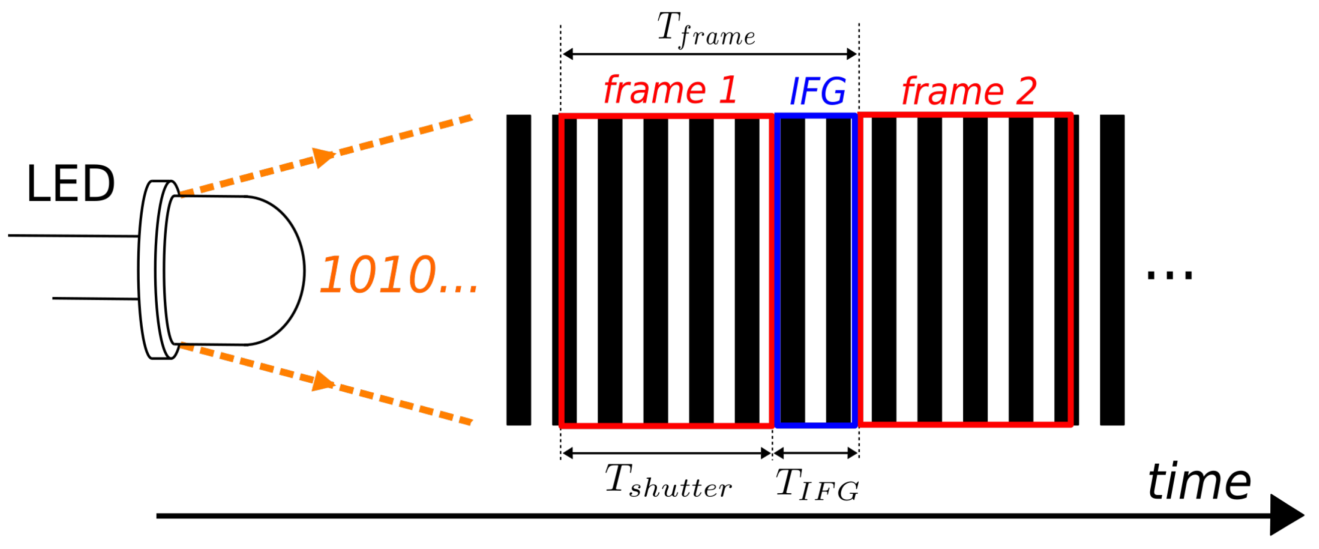
2.1. Rolling Shutter
2.2. Image Conversion
2.3. Region of Interest
2.4. Demodulation
2.5. Binarization
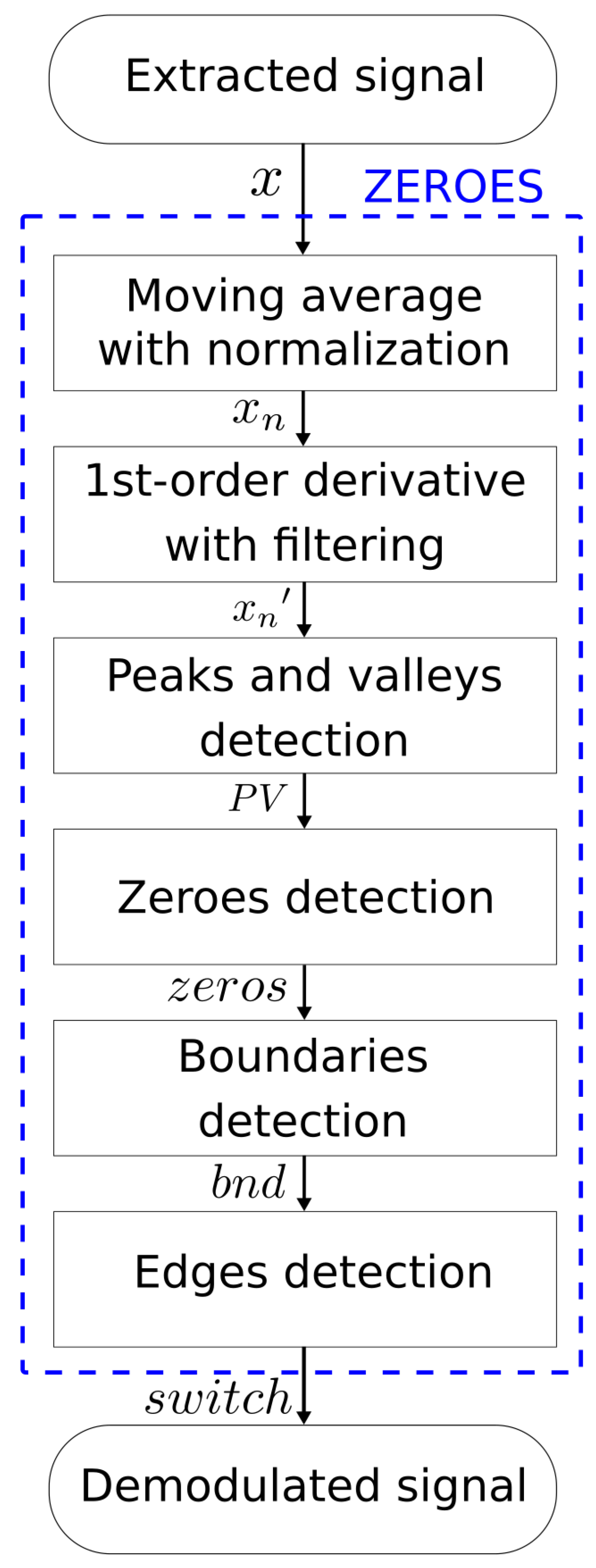
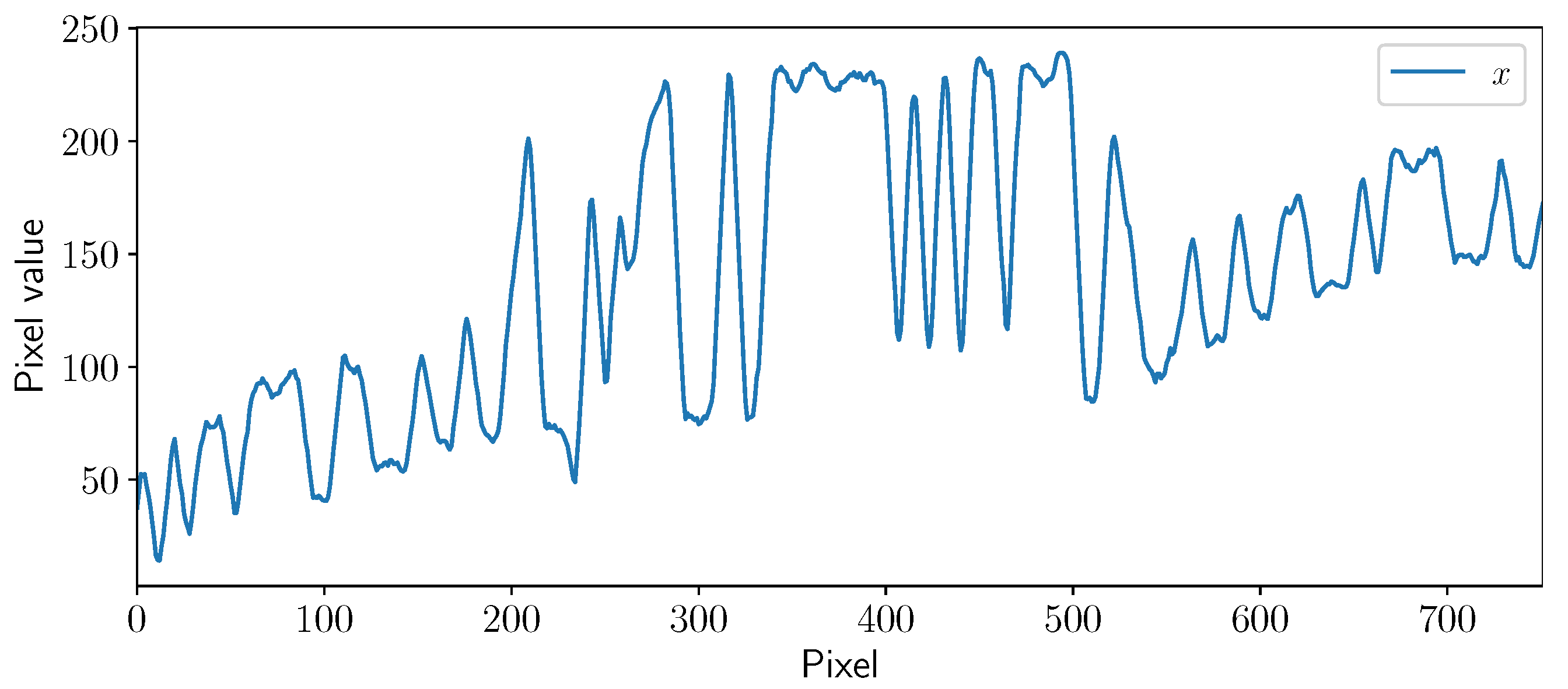
3. Method Description
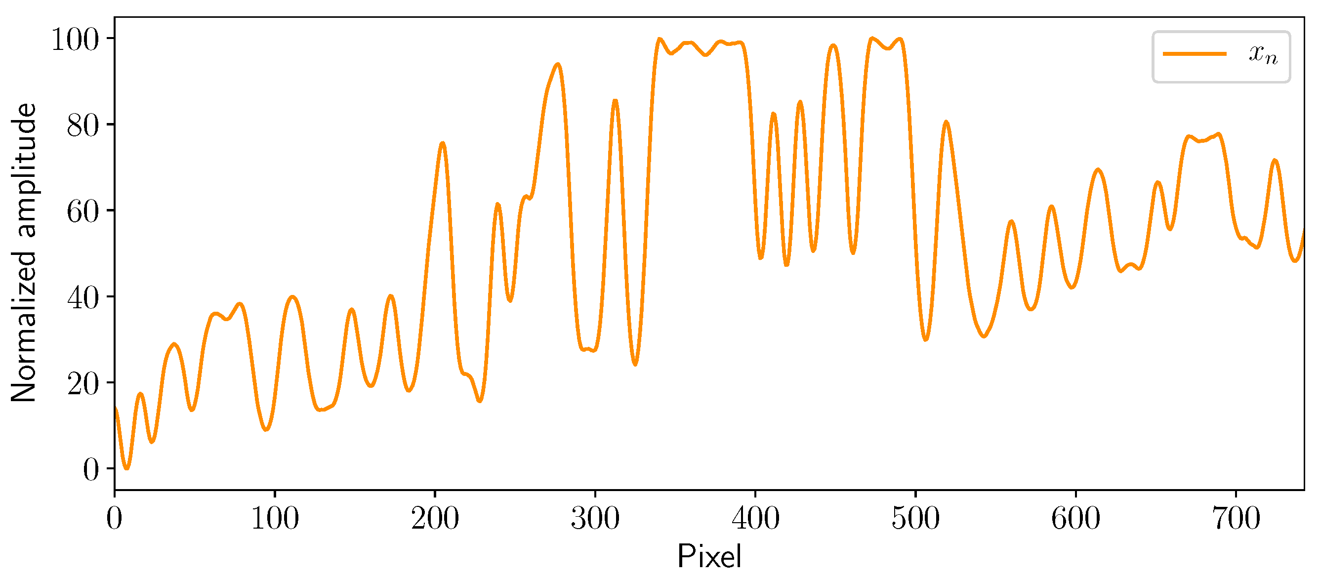
3.1. Moving Average and Normalization
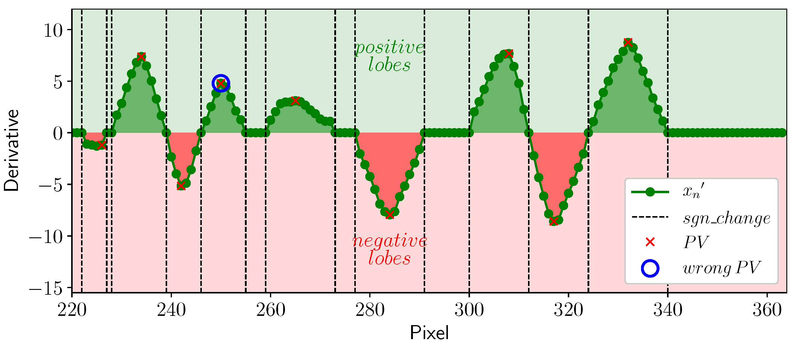
3.2. First-Order Differential Calculation
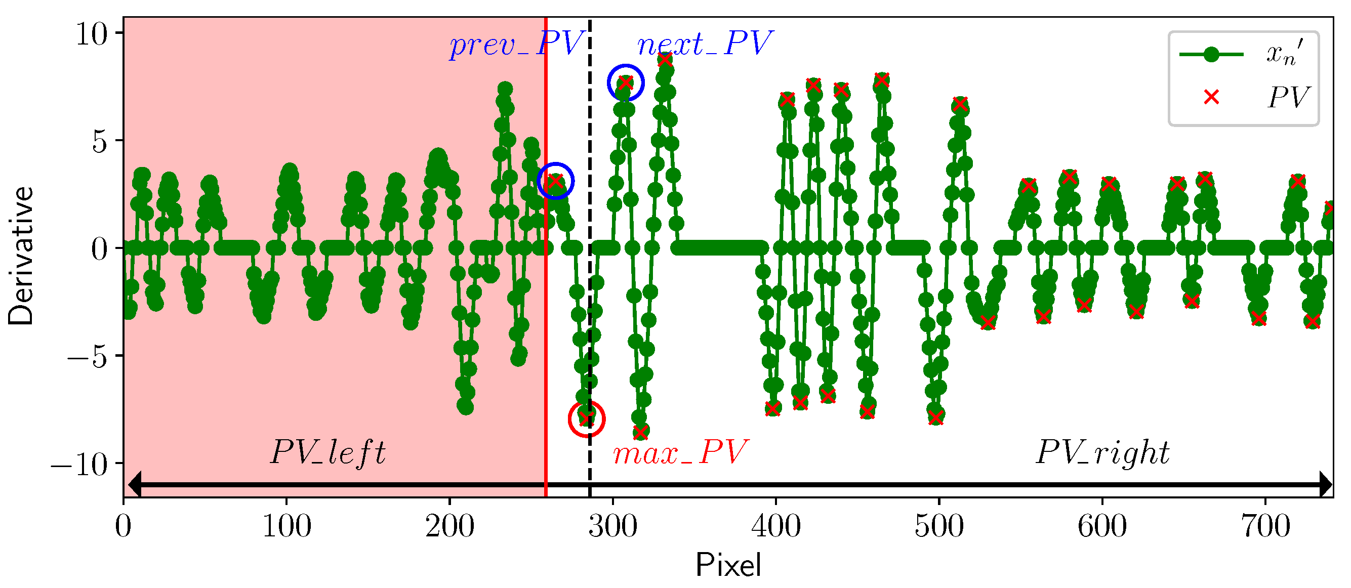
3.3. Detection of Peaks and Valleys
- –
- The amplitude difference between a successive peak/valley.
- –
- The alternating peak/valley pattern.
3.4. Zeros’ Detection
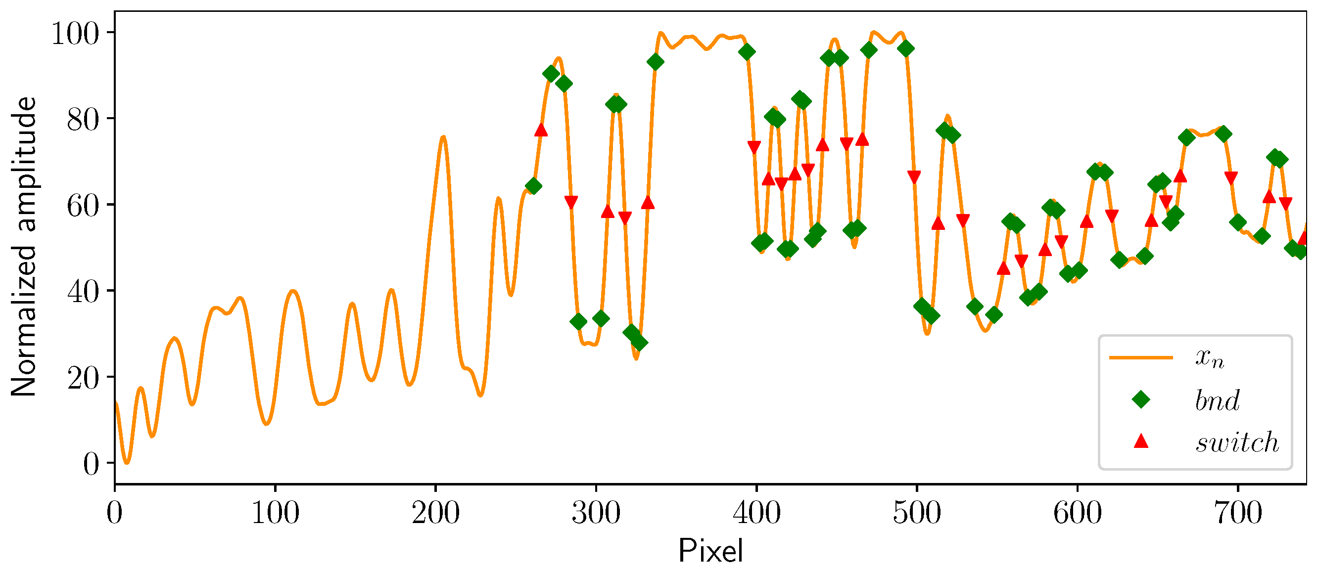
3.5. Boundaries’ Detection
3.6. Edges’ Detection
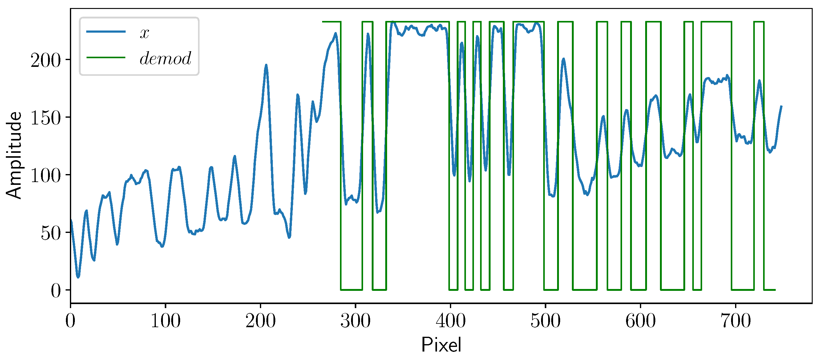
3.7. Demodulation
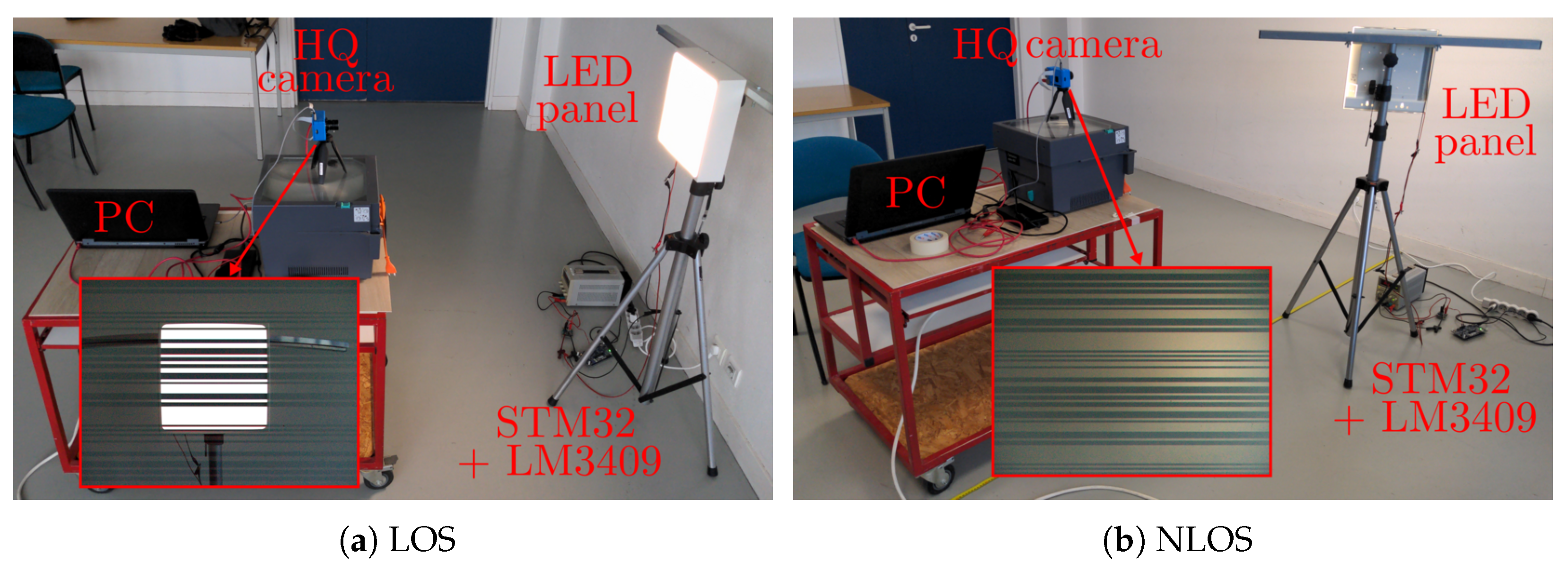
4. Experimental Setup
4.1. Transmission
4.2. Reception
5. Results
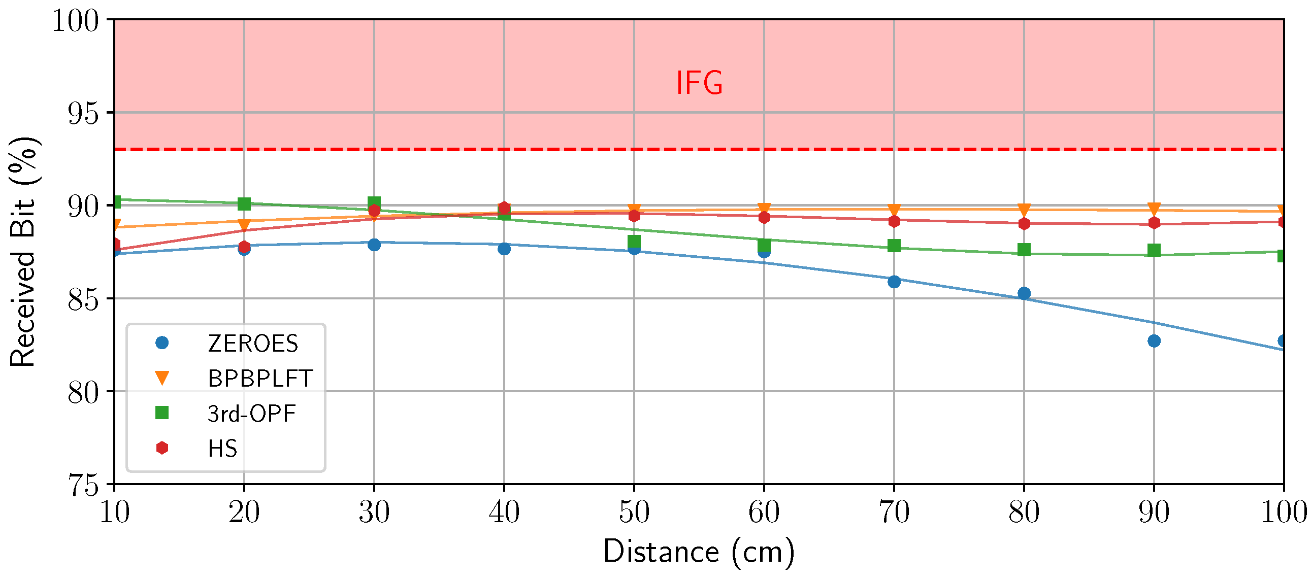
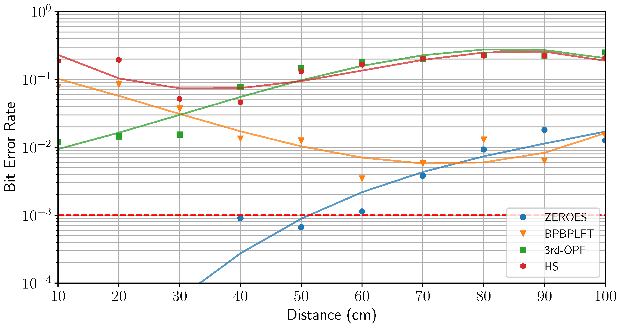
5.1. Line of Sight
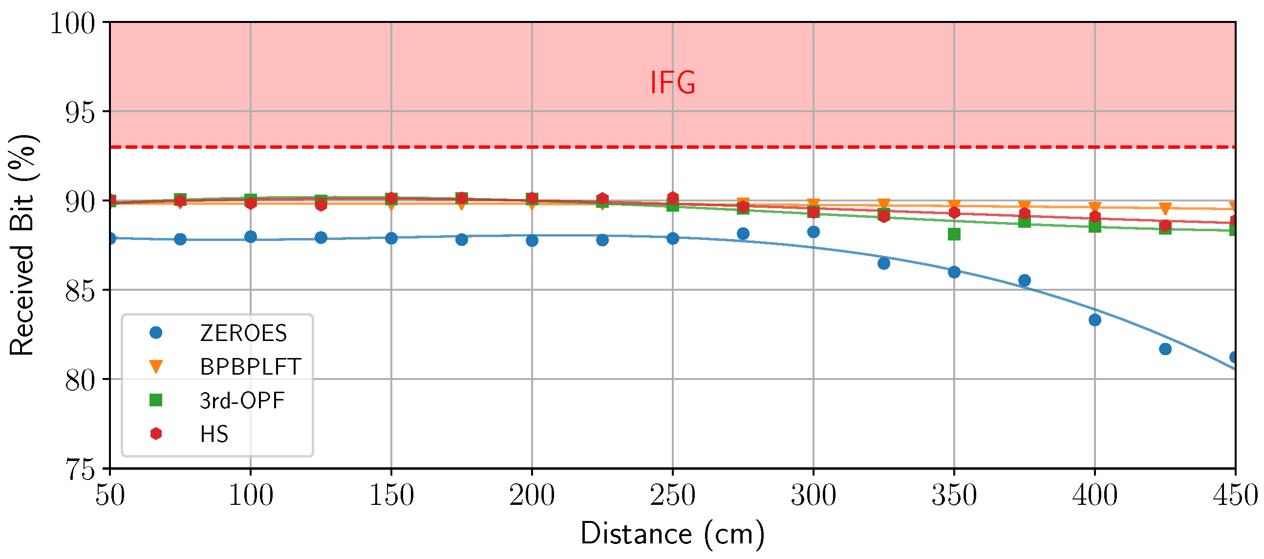
5.2. Non Line of Sight

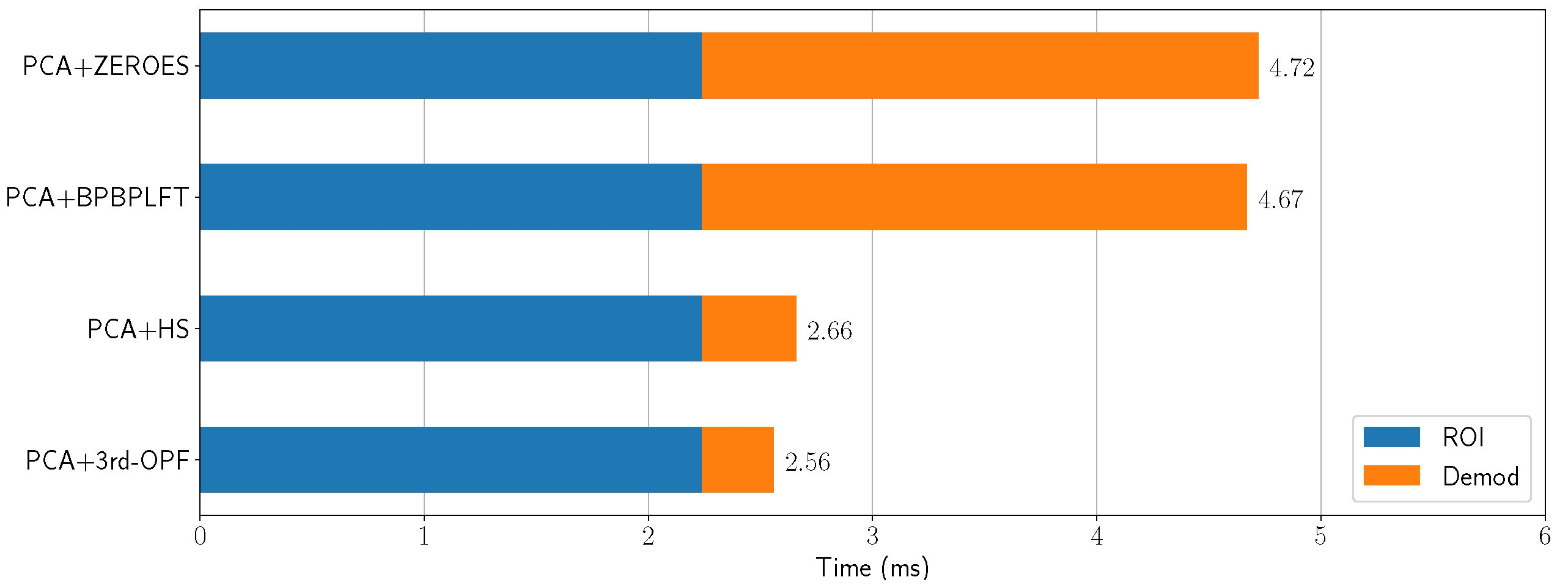
5.3. Execution Time
6. Discussion
Author Contributions
Funding
Data Availability Statement
Conflicts of Interest
Abbreviations
| 3rd-OPF | Third-Order Polynomial Fitting |
| BER | Bit Error Rate |
| BPBPLFT | Boundary Pixel-Based Piecewise Linear Function |
| CCD | Charge-Coupled Device |
| CMOS | Complementary Metal-Oxide Semiconductor |
| ER | Extinction Ratio |
| HS | HyperSight |
| HSV | Hue saturation value |
| IFG | Inter-Frame Gap |
| IoT | Internet of Things |
| ISO | International Standard Organization |
| LED | Light-Emitting Diode |
| LOS | Line Of Sight |
| NLOS | Non Line Of Sight |
| OCC | Optical Camera Communication |
| OOK | On–Off Keying |
| OWC | Optical Wireless Communication |
| PCA | Principal Component Analysis |
| PWM | Pulse-Width Modulation |
| RF | Radio Frequency |
| RGB | Red Green Blue |
| ROI | Region Of Interest |
| SMD | Surface-Mounted Device |
| V2V | Vehicle-to-Vehicle |
| VLC | Visible Light Communication |
| ZEROES | Zeros Evaluation for Robust and Optimal Edges Selection |
References
- Nardelli, A.; Deuschle, E.; de Azevedo, L.D.; Pessoa, J.L.N.; Ghisi, E. Assessment of Light Emitting Diodes technology for general lighting: A critical review. Renew. Sustain. Energy Rev. 2017, 75, 368–379. [Google Scholar] [CrossRef]
- Pons, M.; Valenzuela, E.; Rodríguez, B.; Nolazco-Flores, J.A.; Del-Valle-Soto, C. Utilization of 5G Technologies in IoT Applications: Current Limitations by Interference and Network Optimization Difficulties—A Review. Sensors 2023, 23, 3876. [Google Scholar] [CrossRef] [PubMed]
- Matheus, L.E.M.; Vieira, A.B.; Vieira, L.F.M.; Vieira, M.A.M.; Gnawali, O. Visible Light Communication: Concepts, Applications and Challenges. IEEE Commun. Surv. Tutor. 2019, 21, 3204–3237. [Google Scholar] [CrossRef]
- Chowdhury, M.Z.; Hossan, M.T.; Islam, A.; Jang, Y.M. A Comparative Survey of Optical Wireless Technologies: Architectures and Applications. IEEE Access 2018, 6, 9819–9840. [Google Scholar] [CrossRef]
- Saeed, N.; Guo, S.; Park, K.-H.; Al-Naffouri, T.Y.; Alouini, M.-S. Optical camera communications: Survey, use cases, challenges, and future trends. Phys. Commun. 2019, 37, 100900. [Google Scholar] [CrossRef]
- Danakis, C.; Afgani, M.; Povey, G.; Underwood, I.; Haas, H. Using a CMOS camera sensor for visible light communication. In Proceedings of the 2012 IEEE Globecom Workshops, Anaheim, CA, USA, 3–7 December 2012; pp. 1244–1248. [Google Scholar]
- Durini, D. High Performance Silicon Imaging. Fundamentals and Applications of CMOS and CCD Sensors, 1st ed.; Woodhead Publishing Series in Electronic and Optical Materials; Elsevier Ltd., Woodhead Publishing: Sawston, UK, 2014. [Google Scholar]
- Chow, C.-W.; Chen, C.-Y.; Chen, S.-H. Visible light communication using mobile-phone camera with data rate higher than frame rate. Opt. Express 2015, 23, 26080–26085. [Google Scholar] [CrossRef] [PubMed]
- Kuo, Y.-S.; Pannuto, P.; Hsiao, K.-J. Luxapose: Indoor positioning with mobile phones and visible light. In Proceedings of the 20th Annual International Conference on Mobile Computing and Networking, Maui, HI, USA, 7–11 September 2014. [Google Scholar]
- Hu, X.; Zhang, P.; Sun, Y.; Deng, X.; Yang, Y.; Chen, L. High-Speed Extraction of Regions of Interest in Optical Camera Communication Enabled by Grid Virtual Division. Sensors 2022, 22, 8375. [Google Scholar] [CrossRef] [PubMed]
- Liu, Y.; Chow, C.-W.; Liang, K.; Chen, H.-Y.; Hsu, C.-W.; Chen, C.-Y.; Chen, S.-H. Comparison of thresholding schemes for visible light communication using mobile-phone image sensor. Opt. Express 2016, 24, 1973–1978. [Google Scholar] [CrossRef] [PubMed]
- Zhang, Z.; Zhang, T.; Zhou, J.; Lu, Y.; Qiao, Y. Thresholding Scheme Based on Boundary Pixels of Stripes for Visible Light Communication With Mobile-Phone Camera. IEEE Access 2018, 6, 53053–53061. [Google Scholar] [CrossRef]
- Meng, Y.; Chen, X.; Pan, T.; Shen, T.; Chen, H. HyperSight: A Precise Decoding Algorithm for VLC with Mobile-Phone Camera. IEEE Photonics J. 2020, 12, 7904211. [Google Scholar] [CrossRef]
- Wang, S.; Liu, J.; Zheng, X.; Yang, A.; Song, Y.; Guo, X. Non-Threshold Demodulation Algorithm for CMOS Camera-based Visible Light Communication. In Proceedings of the Opto-Electronics and Communications Conference (OECC), Taipei, Taiwan, 4–8 October 2020; pp. 1–3. [Google Scholar]
- Hossan, T.; Chowdhury, M.Z.; Islam, A.; Jang, Y.M. A Novel Indoor Mobile Localization System Based on Optical Camera Communication. Wirel. Commun. Mob. Comput. 2018, 2018, 9353428. [Google Scholar] [CrossRef]
- Hasan, M.K.; Ali, M.O.; Rahman, M.H.; Chowdhury, M.Z.; Jang, Y.M. Optical Camera Communication in Vehicular Applications: A Review. IEEE Trans. Intell. Transp. Syst. 2022, 23, 6260–6281. [Google Scholar] [CrossRef]
- Teli, S.R.; Matus, V.; Zvanovec, S.; Perez-Jimenez, R.; Vitek, S.; Ghassemlooy, Z. Optical Camera Communications for IoT–Rolling-Shutter Based MIMO Scheme with Grouped LED Array Transmitter. Sensors 2020, 20, 3361. [Google Scholar] [CrossRef] [PubMed]
- Nguyen, H.; Pham, T.L.; Nguyen, H.; Jang, Y.M. Trade-off Communication distance and Data rate of Rolling shutter OCC. In Proceedings of the 11th International Conference on Ubiquitous and Future Networks (ICUFN), Zagreb, Croatia, 2–5 July 2019; pp. 148–151. [Google Scholar]
- De Murcia, M.; Boeglen, H.; Julien-Vergonjanne, A.; Combeau, P. Principal Component Analysis for Robust Region-of-Interest Detection in NLOS Optical Camera Communication. In Proceedings of the 14th International Symposium on Communication Systems, Networks and Digital Signal Processing (CSNDSP), Rome, Italy, 17–19 July 2024; pp. 383–388. [Google Scholar]
- Van, L.T.; Emmanuel, S.; Kankanhalli, M.S. Identifying Source Cell Phone using Chromatic Aberration. In Proceedings of the IEEE International Conference on Multimedia and Expo, Beijing, China, 2–5 July 2007; pp. 883–886. [Google Scholar]
- Duque, A.; Stanica, R.; Rivano, H.; Desportes, A. Decoding methods in LED-to-smartphone bidirectional communication for the IoT. In Proceedings of the Global LIFI Congress (GLC), Paris, France, 8–9 February 2018; pp. 1–6. [Google Scholar]
- Li, X.; Liu, W.; Xu, Z. Design and Implementation of a Rolling Shutter Based Image Sensor Communication System. In Proceedings of the IEEE/CIC International Conference on Communications in China (ICCC Workshops), Chongqing, China, 9–11 August 2020; pp. 253–258. [Google Scholar]
- Yang, Y.; Nie, J.; Luo, J. Reflexcode: Coding with superposed reflection light for led-camera communication. In Proceedings of the 23th ACM MobiCom, Snowbird, UT, USA, 16–20 October 2017. [Google Scholar]
- Holight. CILAOS Product Sheet. Available online: https://www.holight.com/wp-content/uploads/2022/02/CILAOS-2022.pdf (accessed on 1 January 2023).
- Texas Instruments. LM3409, -Q1, LM3409HV, -Q1 P-FET Buck Controller for High-Power LED Drivers. Datasheet, Revised June 2016. Available online: https://www.ti.com/lit/ds/symlink/lm3409.pdf?ts=1728389746781&ref_url=https%253A%252F%252Fwww.ti.com%252Fproduct%252FLM3409 (accessed on 25 September 2024).
- Raspberry Pi. Raspberry Pi High Quality Camera. Datasheet, January 2023. Available online: https://datasheets.raspberrypi.com/hq-camera/hq-camera-product-brief.pdf (accessed on 25 September 2024).
- De Murcia, M. “mdemur01/OCC_ZEROES”, Initial Release, GitLab. Available online: https://gitlab.xlim.fr/mdemur01/occ_zeroes (accessed on 25 September 2024).


| TX Parameters | LOS | NLOS |
|---|---|---|
| LED power | 19.91 W | 19.91 W |
| Panel dimension | 30 × 30 cm | 30 × 30 cm |
| Panel height | 120 cm | 130 cm |
| Panel/wall distance | / | 110 cm |
| Panel/wall orientation | / | 30° |
| Header | 10 bits | 10 bits |
| Payload | 40 bits | 40 bits |
| Data rate | 4 kbps | 4 kbps |
| Modulation | OOK | OOK |
| RX Parameters | LOS | NLOS |
|---|---|---|
| Camera | Raspberry Pi HQ | Raspberry Pi HQ |
| Camera height | 120 cm | 120 cm |
| Camera/LED lateral dist. | / | 105 cm |
| Resolution | 4056 × 3040 | 4056 × 3040 |
| Focal length | 6 mm | 6mm |
| Frame rate | 40 fps | 40 fps |
| Exposure time | 1/16667 s | 1/16667s |
| 23.3 ms | 23.3 ms | |
| ISO | 5769 | 5769 |
| Average ambient light | 1173 lx | 3724 lx |
| 8.25 | 8.25 | |
| , | 4, 100 | 4, 100 |
Disclaimer/Publisher’s Note: The statements, opinions and data contained in all publications are solely those of the individual author(s) and contributor(s) and not of MDPI and/or the editor(s). MDPI and/or the editor(s) disclaim responsibility for any injury to people or property resulting from any ideas, methods, instructions or products referred to in the content. |
© 2024 by the authors. Licensee MDPI, Basel, Switzerland. This article is an open access article distributed under the terms and conditions of the Creative Commons Attribution (CC BY) license (https://creativecommons.org/licenses/by/4.0/).
Share and Cite
De Murcia, M.; Boeglen, H.; Julien-Vergonjanne, A. ZEROES: Robust Derivative-Based Demodulation Method for Optical Camera Communication. Photonics 2024, 11, 949. https://doi.org/10.3390/photonics11100949
De Murcia M, Boeglen H, Julien-Vergonjanne A. ZEROES: Robust Derivative-Based Demodulation Method for Optical Camera Communication. Photonics. 2024; 11(10):949. https://doi.org/10.3390/photonics11100949
Chicago/Turabian StyleDe Murcia, Maugan, Hervé Boeglen, and Anne Julien-Vergonjanne. 2024. "ZEROES: Robust Derivative-Based Demodulation Method for Optical Camera Communication" Photonics 11, no. 10: 949. https://doi.org/10.3390/photonics11100949
APA StyleDe Murcia, M., Boeglen, H., & Julien-Vergonjanne, A. (2024). ZEROES: Robust Derivative-Based Demodulation Method for Optical Camera Communication. Photonics, 11(10), 949. https://doi.org/10.3390/photonics11100949