Single-Pixel Infrared Hyperspectral Imaging via Physics-Guided Generative Adversarial Networks


1
Key Laboratory of Optoelectronic Devices and Detection Technology, School of Physics, Liaoning University, Shenyang 110036, China
2
Center for Quantum Technology Research, Key Laboratory of Advanced Optoelectronic Quantum Architecture and Measurement of Ministry of Education, School of Physics, Beijing Institute of Technology, Beijing 100081, China
*
Authors to whom correspondence should be addressed.
Photonics 2024, 11(2), 174; https://doi.org/10.3390/photonics11020174
Submission received: 5 January 2024
/
Revised: 7 February 2024
/
Accepted: 9 February 2024
/
Published: 12 February 2024
Abstract
:A physics-driven generative adversarial network (GAN) was utilized to demonstrate a single-pixel hyperspectral imaging (HSI) experiment in the infrared spectrum, eliminating the need for extensive dataset training in most data-driven deep neural networks. Within the GAN framework, the physical process of single-pixel imaging (SPI) was integrated into the generator, and its estimated one-dimensional (1D) bucket signals and the actual 1D bucket signals were employed as constraints in the objective function to update the network’s parameters and optimize the generator with the assistance of the discriminator. In comparison to single-pixel infrared HSI methods based on compressive sensing and physics-driven convolution neural networks, our physics-driven GAN-based single-pixel infrared HSI exhibits superior imaging performance. It requires fewer samples and achieves higher image quality. We believe that our physics-driven network will drive practical applications in computational imaging, including various SPI-based techniques.
1. Introduction
Deep learning (DL) [1], originally known as machine learning [2], is a subfield of artificial intelligence, with its origins in the 1950s and 1960s. It aims to mimic human neural networks for intelligent tasks. Nowadays, after several decades of development, it finds applications in healthcare [3,4], natural language processing [5], transportation [6], science and technology [7], and more. Recently, the integration of DL with various optical imaging techniques has opened up extensive prospects for the academic community, significantly enhancing the imaging performance of both traditional and emerging imaging methods, including microscopy [8], ghost imaging (GI) [9], and single-pixel imaging (SPI) [9,10,11,12,13,14], among others. In the field of imaging, the primary DL neural networks are classified into two categories based on their driving types: data-driven (trained) and physics-driven (untrained) neural networks. The former were initially introduced into various imaging fields and image processing, especially in GI or SPI [9,11], showing excellent performance. However, these networks require a large amount of input and output data pairs to train, which results in inherent issues related to generalization [15,16], interpretability, and extended model training time. To address the issues present in data-driven neural networks, the latter, which is based on them and the theory of deep image priors (DIP) [17], has been introduced. The theory of DIP elucidates that a meticulously designed neural network with randomly initialized weights possesses a prior capability biased toward natural images. Currently, this approach has been extensively applied to a variety of optical imaging scenarios [18,19,20,21]. It not only significantly alleviates the issue of generalization in physical imaging at a low computational cost but also further enhances interpretability, and can save a substantial amount of data training time, showcasing promising potential in this field.
Hyperspectral imaging (HSI) is an advanced imaging technique that typically employs multiple well-defined optical bands in a wide spectral range to capture objects, thereby acquiring a set of two-dimensional (2D) images at different wavelengths [22], providing a richer and more extensive set of spectral information compared to RGB and multispectral imaging. Over the last twenty years, HSI has transitioned from its initial use in remote sensing via satellites and aerial platforms to a wide range of applications, encompassing mineral exploration [23], medical diagnostics [24], environmental monitoring [25], and more. However, the need for high-resolution images in HSI to capture fine scene details inevitably leads to substantial data acquisition, increased sampling time (rate), and higher processing and storage costs. The introduction and fusion of compressed sensing (CS) algorithms and SPI provide one of the promising alternative solutions for HSI [26,27,28,29,30,31,32,33], effectively addressing the challenges associated with HSI by utilizing undersampling and single-pixel detection. An illustrative study demonstrates the effectiveness of a CS-based single-pixel HSI method for detecting the chemical composition of targets in the near-infrared spectrum. It highlights the method’s potential for efficient and cost-effective chemical composition detection through high-compression spectral analysis [34]. The other approach is to introduce deep neural networks on the foundation of CS-SPI and other techniques [26,27,28,31,32,33,35,36,37,38,39,40]. A physics-driven convolutional neural network (CNN) was integrated with a single-pixel HSI model to achieve high-quality image reconstruction across a wide range of visible wavelengths at an ultralow sampling rate [26], inspired by the first GI scheme using a physics-driven deep CNN constraint (e.g., GIDC) [41]. Then, a residual degradation learning unfolding network was provided to be applied in compressive spectral imaging [42], and a blind unsupervised neural network was designed to deal with hyperspectral and RGB images, all achieving high-level HSI reconstruction [43]. Furthermore, the integration of computational spectral imaging with physical priors was employed to address the spectral imaging reconstruction challenges [44]. Until now, among various DL networks, only CNNs have been employed in the study of single-pixel HSI, while other potentially more powerful networks, particularly those based on physics-driven principles, remain unexplored.
In this paper, a physics-driven approach based on GAN was proposed to demonstrate a single-pixel infrared HSI experiment by effectively integrating the physical process of SPI and network units of GAN, resulting in the elimination of the need for extensive dataset training in the data-driven deep neural networks. In our study, a comparison was made between our method and the CS algorithm, as well as a physics-driven CNN network, i.e., GIDC, for single-pixel HSI. This comparison was conducted through numerical simulations and experiments, revealing that better imaging quality of the recovered infrared hyperspetral images can be achieved at lower sampling rates (SR) using our approach. Validation was further provided through measurements of peak signal-to-noise ratio (PSNR) and a comparison of the details in reconstructed images under the same conditions.
2. Principle and Method
2.1. Experimental Setup
Our single-pixel HSI experimental apparatus is depicted in Figure 1, which is similar to the typical SPI scheme but with the use of a spectrometer instead of a single-pixel detector. An optical beam from a near-infrared lamp was projected onto an object . The reflected light from the object was imaged onto a digital micromirror device (DMD) via an imaging lens. We employed the Hadamard matrix as the measurement matrix to be loaded onto the DMD (see Figure 1a), where , M denotes the number of modulation pattens (i.e., the number of measurements). After modulation, one reflection beam of the DMD was converged onto a fiber spectrometer and dispersed into several spectral channels. The modulated signals were transformed into one-dimensional (1D) bucket signals of the same length (see Figure 1b) [45], denoted as . To mitigate the impact of environmental noise, we used a differential GI (DGI) algorithm for image reconstruction, utilizing the following formula [46].
where denotes the pixel summation performed on the Hadamard pattern , denotes the ensemble average of the signal . represents the recovered image of pixels. Here, the SR was defined as . The details of the DGI-based single-pixel hyperspectral imaging can be found in Ref. [26], on the basis of which we will introduce our physics-driven GAN framework for its reconstruction in the following.
2.2. Image Reconstruction
After data collection, we would use a physics-driven GAN framework to reconstruct the images.
In the SPI field, data-driven DL algorithms have proven effective in mitigating imaging challenges arising from ultra-low SRs, which is a common issue for conventional CS methods. Regrettably, obtaining sufficient training data is still a challenge in many tasks, and the limited model generalization remains a critical issue in real-world imaging [15,16]. The introduction of physics-driven CNN methods provides new solutions for the model generalization issue, relying solely on the use of mean squared error (MSE) objective function.
Inspired by the above physics-driven mechanism, we proposed a physics-driven GAN approach for single-pixel infrared HSI reconstruction, where the physical process was integrated with the generator. The method optimized the parameters by using both the MSE objective function and the adversarial objective function, thereby enabling the recovery of high-quality images without the need for dataset training. This physics-driven GAN-based image reconstruction method could be formulated as a min–max optimization problem (see Refs. [47,48]).
Here, represents the mathematical expectation of r (), z stands for the speckle map as the random input, is the value function of the GAN, indicates the generator model for generating the estimated 1D bucket signals , and denotes the discriminator model for distinguishing between the estimated 1D bucket signal and the actual 1D bucket signal . The discriminator needed to maximize its discriminative ability between (fake) and (real). The primary role of the GAN used here was to adjust the parameters of to make the estimated signal much closer to the real measured signal . When and are very close to each other, at this point is the final output reconstructed image (Figure 2).
As mentioned above, we would optimize the parameters of through the objective function, which consisted of parts from both the MSE objective function and the adversarial objective function. The MSE objective function was defined as follows [48,49]:
In principle, there are infinitely many that can satisfy the objective function. Hence, it is necessary to add prior information about the image to select a feasible solution from all options. However, existing work empirically demonstrated that an appropriately designed neural network with randomly initialized weights possesses a prior bias towards natural images [18,19,20,21]. Therefore, we also employed the randomly initialized prior in our generator network.
Next, we would use the objective function to optimize the network parameters. The purpose of the adversarial constraint was to make the output much closer to the real data. Since this objective function was related to the discriminator network, we minimized the negative log-likelihood of the discriminator, thereby increasing the probability that the generator’s output values become close to . The adversarial objective function could be written as [49]
where is the output of the generator and signifies the probability that the estimated 1D bucket signal and the actual 1D bucket signal were very close to each other. The final objective function was
The generator network parameters could be optimized through the following formula:
where in represents the optimal parameters for the generator. By minimizing the objective function in Equation (6), the optimal parameters for the generator were obtained, making much closer to . At this point, the reconstruction was at its best.
It is worth noting that SPI-based GAN [48] also employs GAN but reconstructs images through the following formula:
where is the ground truth image in the dataset. The SPI-based GAN learns the mapping from low-quality images to high-quality images in the dataset , , to optimize the parameters of the generator . Conversely, our proposed method updates the parameters in the neural network through the objective function constrained by and , which can be seen as the combination between the GI physical model and . In contrast, by using our approach, the reconstructed image was obtained without any dataset training, where denoted the reconstructed image. It is also noteworthy that the input of our proposed neural network can be a rough image restored by any traditional GI algorithm, or even a random noise image . Hereinafter, we used for convenience.
The principle process of the proposed method is described as follows (see Figure 2). Step 1: the measured 1D bucket signal is input into the discriminator, which applies a cross-entropy objective function for solving the maximum and minimum problem (Equation (2)). The parameters of the discriminator are updated by using the backpropagation algorithm, enhancing its ability to distinguish between real and fake data. Step 2: a random noise image z is input into the untrained generator to produce the image , which is then converted into a 1D bucket signal I by using the modulation patterns H, i.e., . The objective function of the generator (Equation (6)) is computed and used to guide the update of the generator’s parameters , also by employing the backpropagation algorithm. We need to execute Steps 1 and 2 in turn. By this means, the iterative process of the generative adversarial network can be regarded as a dynamic game process, where the generator and discriminator improve their performance through mutual antagonism and cooperation. Alternate iterations until the generator and discriminator reach an ideal performance level or the number of iterations reaches the set value.
The network framework of the proposed method is shown in Figure 3, where the generator consists of two processes: up-sampling and down-sampling. In down-sampling process, there are convolution blocks ( convolution (stride 1) + batch normalization (BN) + leaky ReLU) and max pooling operations (stride 2). The up-sampling involves deconvolution blocks ( deconvolution (stride 2) + BN + leaky ReLU). The discriminator comprises four fully connected layers, each of , ending with a sigmoid function. The number N in the generator network is set to 64. Both networks use a learning rate (LR) of 0.001 and employ leaky ReLU as the activation function. Here, an Adam optimizer is used to optimize the network parameters. In the experiments, we utilized an NVIDIA RTX2060 graphics card with a memory of 16 GB and an Intel i7-10875H processor.
3. Results and Discussion
In order to verify the effectiveness of our method, we conducted a comparison with the CS and GIDC algorithms through simulations and experiments. We employed the peak signal-to-noise ratio (PSNR) (a commonly used metric) and structural similarity (SSIM) index to quantitatively analyze the reconstruction quality. We then compared the differences between the reconstructed image and ground truth image. The formula for calculating PSNR is
where is the maximum value of the image, and MSE is expressed by
Here, and represent the ground truth image and the reconstructed image, respectively, while a and b denote the row and column coordinates of images. The SSIM is a criterion for evaluating the similarity between two images and is commonly used in the field of image processing to assess image quality. It is based on the computation of three terms that compare the luminance, contrast, and structure of the test and reference images. The formula for the SSIM can be written as
where J and K are the two images to be compared, and are their average luminances, and are their standard deviations, is the covariance between both images, and and are small constants for avoiding a zero denominator. The value of the SSIM ranges from −1 to 1, where 1 indicates perfect similarity between two images.
3.1. Simulations
Since each wavelength channel in the single-pixel HSI is discrete, we first performed the numerical simulation for a single spectral channel by using our physics-based GAN. Here, a building image of pixels (see Figure 4(a1)) was used as the target to be imaged, which was considered as the image to be imaged onto the DMD. We applied modulation patterns to generate the 1D bucket signal (which was of in length), leading to the SR %. The LR was set to 0.001. According to our proposed scheme, the physical process was simulated as follows. The Hadamard patterns were rearranged by following the Harr wavelet transform ranking method [50]. By this means, each modulated image was summed pixel by pixel to obtain the 1D bucket signal (Figure 1b), which was fed into the discriminator, while the random noise map was treated as the input of the generator. By following the steps in the principle section and optimizing the parameters using the objective function (see Equations (2) and (7)), the optimal generator and reconstructed image were obtained. We set the number of iterations to 10, 50, 100, and 150 and obtained their corresponding reconstructed images, as shown in Figure 4(b1). Evidently, the image quality improves with the increase in the number of iterations, proven by PSNRs and SSIMs. When the number of iterations is less than 50, the quality improvement is obvious, and, when the number of iterations is greater than 150, the quality improvement tends to be saturated as the network tends to converge at this point. This is explained through Figure 4(c1,d1). It can be observed that the loss functions of the generator and discriminator tend to stabilize around 150, indicating that the network has reached convergence.
To compare the performance of our network with other algorithms, another simulation was performed. Another boat image of pixels (see Figure 4(a2)) was used as the target, and its corresponding noisy image was shown in Figure 4(b2). The CS-based SPI (with well-known total variation augmented Lagrangian alternating direction (TVAL3) [51] algorithm) and SPI-based CNN (with commonly used “GI using deep neural network constraint” (GIDC) [26,41] algorithm) were utilized for reconstruction under the same conditions. The SR varied from 5% to 30%, and the corresponding results for the three methods are shown in Figure 4(c2–e2). The image quality improved as the SR increased. For each given SR, our method performed the best, followed by GIDC and TAVL3. Based on the visual analysis of Figure 4(c2–e2), it becomes apparent that the utilization of TVAL3 and GIDC resulted in a notable decline in image quality at an SR of 10%. On the contrary, even when the SR is reduced to 5%, images restored using our proposed method still remain distinguishable for the target.
In order to perform a quantitative analysis of the image quality, the PSNRs and SSIMs of images reconstructed by the above three methods at various SRs were also calculated and provided in Figure 4(c2–e2). At different given SRs, the PSNR and SSIM of our proposed method surpass those of GIDC and TVAL3. As the SR decreased, the PSNRs of the images recovered by all three methods showed a decreasing trend, which was consistent with the trend indicated in the images. At an SR of 5%, the PSNR and SSIM of our method reached 17.21 dB and 0.39, respectively, while the PSNR and SSIM of the TVAL3 and GIDC methods were only (15.74 dB, 0.18) and (14.48 dB, 0.36), respectively, almost equivalent to the images reconstructed by GIDC and TVAL3 at an SR of 10%. Based on the above analysis, it was evident that our method was proficient at reconstructing target images even at extremely low SRs, and it consistently yielded significantly better image quality compared with the other two methods. This exceptional performance underscored the promising potential of our proposed method for practical imaging scenarios.
3.2. Experiments
In the previous subsection, we demonstrated the outstanding performance of our physics-driven GAN method in SPI through a comparative analysis with two other image reconstruction techniques in numerical simulations. In this subsection, we continue to verify the performance of our physics-driven GAN in infrared single-pixel HSI experiments. The experimental setup is shown in Figure 1, where we used a toy train model as the imaging target. The hardware configuration is shown in Table 1. An infrared beam emitted from a lamp with a wavelength range of 880 nm to 1600 nm illuminated the toy train, which was then imaged onto the DMD (ViALUXV-7001) through an imaging lens ( cm) with a focal length of 60 mm. Then, after modulation, one of the beams reflected from the DMD passed through a collecting lens onto an infrared spectrometer (FUXIAN, NIR17+Px), and the recorded signal was dispersed into 512 spectral channels with a step of nm. All the bucket signals, denoted as , extracted from the spectrum were stored.
In our physics-driven GAN, a random noise image z was used as the input for the generator, the result of which was multiplied by modulation patterns to produce . Simultaneously, the 1D bucket signals of 512 distinct wavelengths were sequentially fed into the discriminator network. The SR was set as 10% and 20%. Upon the network’s completion, a total of 512 near-infrared hyperspectral images were sequentially reconstructed. For comparative purposes, we utilized the TVAL3 and GIDC methods to reconstruct an equivalent set of 512 near-infrared hyperspectral images under identical conditions. To ensure a concise presentation, we deliberately selected only 14 images for each method, spaced at 50 nm intervals. These selected images are showcased in Figure 5 to underscore the key findings. As the SR increases, the quality of the images improves. For each given SR, our method outperforms the others, while, at 20% SR (Figure 5a), the GIDC method successfully reconstructed the train model image, but there were clarity issues in the wavelength range of 900 nm to 1000 nm and 1200 nm to 1400 nm. Although the GIDC method reconstructed clearer train model images, it still struggled with clarity and contrast in the 1000 nm to 1050 nm and 1300 nm to 1350 nm ranges. In contrast, our proposed method consistently produced images with significantly enhanced contrast and clarity across all wavelength ranges. At 10% SR (Figure 5b), the images reconstructed by the TVAL3 and GIDC methods were indistinguishable and had contrast issues, whereas our method could reconstruct images with better contrast and clarity. Consequently, when compared to the other two methods, our proposed approach demonstrated superior imaging performance at low SRs in the single-pixel infrared HSI scheme.
To further assess the performance of our proposed single-pixel infrared HSI method, we conducted a quantitative analysis. We obtained reconstructed images at various wavelengths by using three different methods. As shown in Figure 6a, once the light intensity had been normalized, pixel ① corresponded to the light transmission portion of the reconstructed object image, with an intensity of 1, while pixel ② corresponded to the non-light transmission portion of the background image, with an intensity of 0. To evaluate the reconstructed image’s quality, we compared the light intensity differences at the specific pixels for each method with actual light intensity. A closer match between the pixel values of the reconstructed image and actual values indicated a more accurate imaging performance. By this means, it allowed us to quantitatively evaluate and compare different methods in terms of reconstructed image quality, providing a more precise assessment of our proposed method’s performance in single-pixel infrared HSI applications.
The specific comparison results are presented in Figure 6b (corresponding to pixel ①) and Figure 6c (corresponding to pixel ②). The black curve, red curve, and blue curve represent the performance of the reconstructed images by the TVAL3 method, GIDC method, and the method we proposed, respectively, under the condition of an SR = 20%. It is clearly observed that, at pixel ①, the light intensity values obtained by the TVAL3 method are far from the actual light intensity x = 1 across all wavelengths, while the GIDC method performs better than TVAL3, but not as well as the method we proposed. This can be observed from the blue curve, which is significantly higher than the other two curves and approaching x = 1. Similarly, at pixel ②, the light intensity values measured by the GIDC method are more accurate than those by TVAL3, but the light intensity measured by our proposed method is closer to the actual value x = 0 at different wavelengths. It is worth mentioning that our method does not show a significant change in intensity at different wavelengths for the selected pixel location ① (see Figure 6b) because the light intensity at this pixel location is within the object part, where the light intensity is relatively strong and uniform. Moreover, this subfigure is mainly to show that the reconstruction of our method is superior compared to the TVAL3 and GIDC methods. When at the pixel position ② in the background part (see Figure 6c), the reconstructed grayscale values of our method show significant changes at different wavelengths. Therefore, the train object we selected in our experiments has different spectral absorbance in each respective spectral regime. Here, as a demonstration of the principle, and without loss of generality, the used train object has proven that our method is effective for the general complex object. Therefore, these results once again corroborate the significant advantage of the method we proposed in object reconstruction, showcasing its robust reconstructive performance. The data provided above lend strong support and validation to the powerful performance of the method we proposed in the domain of single-pixel hyperspectral imaging.
To further compare the stability and efficiency of our proposed method and the GIDC method, both methods underwent 450 iterations at a 20% SR. Eight images from each method were selected as shown in the following Figure 7. In a large number of experiments, the images reconstructed by GIDC (Figure 7a) from iterations 10 to 50 were indistinguishable, and the quality of the reconstructed images deteriorated after 250 iterations. In contrast, our method (Figure 7b) produced reconstructed images with significantly improved contrast and clarity after just 30 iterations, and the quality of the reconstructed images did not decline with an increase in thea number of iterations. Compared to GIDC, our method demonstrates more stable and efficient image quality in the single-pixel infrared HSI scheme.
In the preceding paragrabphs, we compared the experimental results of three different methods, demonstrating convincingly that our proposed physics-driven GAN could achieve better image quality under the same conditions. The configuration of network parameters also plays a crucial role in the effectiveness of image recovery. Therefore, we further demonstrated this point by investigating the network parameters. Here, we set SR to 20% and the number of network iterations as 120, spaced at 20 intervals. In our network, the LR is an important parameter. It could be observed from Figure 8, with the increase in the number of iterations, that the image quality of the reconstructions under different LRs using our proposed method improves. It can be observed that images reconstructed with an LR of 0.00001 remain blurry within 120 iterations (Figure 8a), while those reconstructed with an LR of 0.0001 show improved image quality after 40 iterations(Figure 8b), although they are still blurry at 20 iterations. In contrast, images reconstructed with an LR of 0.001 reach high quality just after 20 iterations(Figure 8c). However, when the LR is increased to 0.01, the reconstructed images again become blurry within 120 iterations(Figure 8d). This is because setting the LR at 0.0001 is too low, which leads to a slower convergence of the generator’s loss function, and thus requires more iterations. At an LR of 0.0001, the convergence speed increased, requiring fewer iterations. When the LR was 0.001, the convergence was the fastest, requiring the least number of iterations. However, when the LR reaches 0.01, images cannot be clearly reconstructed. The optimization process constantly overshoots the minimum points, making it difficult for the model to find the optimal point of the loss function. This leads to an inability to clearly reconstruct images. Therefore, appropriate setting of the LR is crucial not only for image quality but also for reducing the number of iterations, accelerating network convergence, and improving imaging speed.
A comparison of computation time (which characterizes the computational complexity) using different methods at various sampling rates is provided in Table 2. We can see from the results that the CS method runs the fastest, followed by the GIDC method, and our proposed method is the slowest. Since both the GIDC approach and our method involve iterative processes, they require more time than the CS method. Meanwhile, our method requires alternating iterations and updates for the generator and discriminator, leading to a longer computation time than the GIDC method. Our future work will focus on optimizing the network structure to reduce computation time.
4. Conclusions
We proposed a physics-driven GAN framework, which was successfully applied to single-pixel infrared HSI. Over 500 spectral images of the imaging target have been achieved at a 20% SR. The fusion of physical processes and the GAN primarily exhibits two advantages. First, through 1D bucket signals, we are able to impose constraints on the MSE objective function and adversarial objective function of the GAN, thereby updating the network parameters and eliminating the dependency on datasets for training, which significantly enhances the generalization capability of the network. Second, the constraints of multi-objective functions contribute to a notable improvement in the quality of the reconstructed images. Our numerical simulations and single-pixel infrared HSI experiments have provided strong evidence for the excellent performance of the physics-driven GAN in achieving high-quality image reconstruction at low SRs. This forms a robust foundation for its application in areas such as infrared spectral detection. Although such a configuration might incur some time consumption, it enables a broader spectral detection range and lower costs. Although our proposed method significantly reduces the time required for data-driven network training, it still requires more computation time compared to commonly used CS algorithms. The feasible approaches to enhance the computational efficiency of the proposed scheme include designing a more optimal neural network architecture, adopting improved initialization strategies, and utilizing a more advanced computing platform. Another practical challenge is that the image reconstruction method of combining untrained neural networks with specific imaging physical processes requires more accurate imaging models, posing an extremely challenging task in computational spectral imaging fields.
Author Contributions
Conceptualization, D.-Y.W. and X.-H.C.; Methodology, D.-Y.W.; Validation, S.-H.B. and X.-H.C.; Writing—original draft preparation, D.-Y.W.; Writing—review and editing, X.-H.C. and W.-K.Y.; Data curation, D.-Y.W. and S.-H.B.; Supervision, X.-H.C. and W.-K.Y.; Funding acquisition, X.-H.C. and W.-K.Y. All authors have read and agreed to the published version of the manuscript.
Funding
National Key Research and Development Program of China (2018YFB0504302); Beijing Natural Science Foundation (4222016); National Defence Science and Technology Innovation Zone (23-TQ09-41-TS-01-011).
Institutional Review Board Statement
Not applicable.
Informed Consent Statement
Not applicable.
Data Availability Statement
Data are contained within the article.
Conflicts of Interest
The authors declare no conflicts of interest.
References
- Sarker, I.H. Deep learning: A comprehensive overview on techniques, taxonomy, applications and research directions. SN Comput. Sci. 2021, 2, 420. [Google Scholar] [CrossRef]
- Jordan, M.I.; Mitchell, T.M. Machine learning: Trends, perspectives, and prospects. Science 2015, 349, 255–260. [Google Scholar] [CrossRef]
- Miotto, R.; Wang, F.; Wang, S.; Jiang, X.; Dudley, J.T. Deep learning for healthcare: Review, opportunities and challenges. Briefings Bioinform. 2018, 19, 1236–1246. [Google Scholar] [CrossRef]
- Rahman, A.; Hossain, M.S.; Muhammad, G.; Kundu, D.; Debnath, T.; Rahman, M.; Khan, M.S.I.; Tiwari, P.; Band, S.S. Federated learning-based AI approaches in smart healthcare: Concepts, taxonomies, challenges and open issues. Clust. Comput. 2023, 26, 2271–2311. [Google Scholar] [CrossRef]
- Lauriola, I.; Lavelli, A.; Aiolli, F. An introduction to deep learning in natural language processing: Models, techniques, and tools. Neurocomputing 2022, 470, 443–456. [Google Scholar] [CrossRef]
- Kashyap, A.A.; Raviraj, S.; Devarakonda, A.; Nayak K, S.R.; KV, S.; Bhat, S.J. Traffic flow prediction models–a review of deep learning techniques. Cogent Eng. 2022, 9, 2010510. [Google Scholar] [CrossRef]
- Choudhary, K.; DeCost, B.; Chen, C.; Jain, A.; Tavazza, F.; Cohn, R.; Park, C.W.; Choudhary, A.; Agrawal, A.; Billinge, S.J.; et al. Recent advances and applications of deep learning methods in materials science. npj Comput. Mater. 2022, 8, 59. [Google Scholar] [CrossRef]
- Ragone, M.; Shahabazian-Yassar, R.; Mashayek, F.; Yurkiv, V. Deep learning modeling in microscopy imaging: A review of materials science applications. Prog. Mater. Sci. 2023, 138, 101165. [Google Scholar] [CrossRef]
- Lyu, M.; Wang, W.; Wang, H.; Wang, H.; Li, G.; Chen, N.; Situ, G. Deep-learning-based ghost imaging. Sci. Rep. 2017, 7, 17865. [Google Scholar] [CrossRef] [PubMed]
- Song, K.; Bian, Y.; Wu, K.; Liu, H.; Han, S.; Li, J.; Tian, J.; Qin, C.; Hu, J.; Xiao, L. Single-pixel imaging based on deep learning. arXiv 2023, arXiv:2310.16869v1. [Google Scholar]
- Hoshi, I.; Takehana, M.; Shimobaba, T.; Kakue, T.; Ito, T. Single-pixel imaging for edge images using deep neural networks. Appl. Opt. 2022, 61, 7793–7797. [Google Scholar] [CrossRef] [PubMed]
- Liu, X.; Han, T.; Zhou, C.; Huang, J.; Ju, M.; Xu, B.; Song, L. Low sampling high quality image reconstruction and segmentation based on array network ghost imaging. Opt. Express 2023, 31, 9945–9960. [Google Scholar] [CrossRef] [PubMed]
- Rizvi, S.; Cao, J.; Hao, Q. Deep learning based projector defocus compensation in single-pixel imaging. Opt. Express 2020, 28, 25134–25148. [Google Scholar] [CrossRef] [PubMed]
- Rizvi, S.; Cao, J.; Zhang, K.; Hao, Q. Improving imaging quality of real-time Fourier single-pixel imaging via deep learning. Sensors 2019, 19, 4190. [Google Scholar] [CrossRef] [PubMed]
- Alzubaidi, L.; Bai, J.; Al-Sabaawi, A.; Santamaría, J.; Albahri, A.; Al-dabbagh, B.S.N.; Fadhel, M.A.; Manoufali, M.; Zhang, J.; Al-Timemy, A.H.; et al. A survey on deep learning tools dealing with data scarcity: Definitions, challenges, solutions, tips, and applications. J. Big Data 2023, 10, 46. [Google Scholar] [CrossRef]
- Brigato, L.; Iocchi, L. A Close Look at Deep Learning with Small Data. arXiv 2020, arXiv:2003.12843v1. [Google Scholar]
- Ulyanov, D.; Vedaldi, A.; Lempitsky, V. Deep image prior. In Proceedings of the IEEE Conference on Computer Vision and Pattern Recognition, Salt Lake City, UT, USA, 18–23 June 2018; pp. 9446–9454. [Google Scholar]
- Wang, F.; Bian, Y.; Wang, H.; Lyu, M.; Pedrini, G.; Osten, W.; Barbastathis, G.; Situ, G. Phase imaging with an untrained neural network. Light. Sci. Appl. 2020, 9, 77. [Google Scholar] [CrossRef]
- Lin, J.; Yan, Q.; Lu, S.; Zheng, Y.; Sun, S.; Wei, Z. A compressed reconstruction network combining deep image prior and autoencoding priors for single-pixel imaging. Photonics 2022, 9, 343. [Google Scholar] [CrossRef]
- Gelvez-Barrera, T.; Bacca, J.; Arguello, H. Mixture-net: Low-rank deep image prior inspired by mixture models for spectral image recovery. Signal Process. 2023, 216, 109296. [Google Scholar] [CrossRef]
- Bostan, E.; Heckel, R.; Chen, M.; Kellman, M.; Waller, L. Deep phase decoder: Self-calibrating phase microscopy with an untrained deep neural network. Optica 2020, 7, 559–562. [Google Scholar] [CrossRef]
- Garini, Y.; Young, I.T.; McNamara, G. Spectral imaging: Principles and applications. Cytom. Part A J. Int. Soc. Anal. Cytol. 2006, 69, 735–747. [Google Scholar] [CrossRef]
- Deng, K.; Zhao, H.; Li, N.; Wei, W. Identification of minerals in hyperspectral imagery based on the attenuation spectral absorption index vector using a multilayer perceptron. Remote Sens. Lett. 2021, 12, 449–458. [Google Scholar] [CrossRef]
- Barberio, M.; Benedicenti, S.; Pizzicannella, M.; Felli, E.; Collins, T.; Jansen-Winkeln, B.; Marescaux, J.; Viola, M.G.; Diana, M. Intraoperative guidance using hyperspectral imaging: A review for surgeons. Diagnostics 2021, 11, 2066. [Google Scholar] [CrossRef]
- Stuart, M.B.; McGonigle, A.J.; Willmott, J.R. Hyperspectral imaging in environmental monitoring: A review of recent developments and technological advances in compact field deployable systems. Sensors 2019, 19, 3071. [Google Scholar] [CrossRef]
- Wang, C.H.; Li, H.Z.; Bie, S.H.; Lv, R.B.; Chen, X.H. Single-pixel hyperspectral imaging via an untrained convolutional neural network. Photonics 2023, 10, 224. [Google Scholar] [CrossRef]
- Magalhães, F.; Abolbashari, M.; Araújo, F.M.; Correia, M.V.; Farahi, F. High-resolution hyperspectral single-pixel imaging system based on compressive sensing. Opt. Eng. 2012, 51, 071406. [Google Scholar] [CrossRef]
- Welsh, S.S.; Edgar, M.P.; Bowman, R.; Jonathan, P.; Sun, B.; Padgett, M.J. Fast full-color computational imaging with single-pixel detectors. Opt. Express 2013, 21, 23068–23074. [Google Scholar] [CrossRef] [PubMed]
- Radwell, N.; Mitchell, K.J.; Gibson, G.M.; Edgar, M.P.; Bowman, R.; Padgett, M.J. Single-pixel infrared and visible microscope. Optica 2014, 1, 285–289. [Google Scholar] [CrossRef]
- August, Y.; Vachman, C.; Rivenson, Y.; Stern, A. Compressive hyperspectral imaging by random separable projections in both the spatial and the spectral domains. Appl. Opt. 2013, 52, D46–D54. [Google Scholar] [CrossRef] [PubMed]
- Hahn, J.; Debes, C.; Leigsnering, M.; Zoubir, A.M. Compressive sensing and adaptive direct sampling in hyperspectral imaging. Digit. Signal Process. 2014, 26, 113–126. [Google Scholar] [CrossRef]
- Tao, C.; Zhu, H.; Wang, X.; Zheng, S.; Xie, Q.; Wang, C.; Wu, R.; Zheng, Z. Compressive single-pixel hyperspectral imaging using RGB sensors. Opt. Express 2021, 29, 11207–11220. [Google Scholar] [CrossRef] [PubMed]
- Yi, Q.; Heng, L.Z.; Liang, L.; Guangcan, Z.; Siong, C.F.; Guangya, Z. Hadamard transform-based hyperspectral imaging using a single-pixel detector. Opt. Express 2020, 28, 16126–16139. [Google Scholar] [CrossRef] [PubMed]
- Gattinger, P.; Kilgus, J.; Zorin, I.; Langer, G.; Nikzad-Langerodi, R.; Rankl, C.; Gröschl, M.; Brandstetter, M. Broadband near-infrared hyperspectral single pixel imaging for chemical characterization. Opt. Express 2019, 27, 12666–12672. [Google Scholar] [CrossRef] [PubMed]
- Mur, A.L.; Montcel, B.; Peyrin, F.; Ducros, N. Deep neural networks for single-pixel compressive video reconstruction. In Unconventional Optical Imaging II; SPIE: Bellingham, WA, USA, 2020; Volume 11351, pp. 71–80. [Google Scholar]
- Kim, Y.C.; Yu, H.G.; Lee, J.H.; Park, D.J.; Nam, H.W. Hazardous gas detection for FTIR-based hyperspectral imaging system using DNN and CNN. In Electro-Optical and Infrared Systems: Technology and Applications XIV; SPIE: Bellingham, WA, USA, 2017; Volume 10433, pp. 341–349. [Google Scholar]
- Heiser, Y.; Oiknine, Y.; Stern, A. Compressive hyperspectral image reconstruction with deep neural networks. In Big Data: Learning, Analytics, and Applications; SPIE: Bellingham, WA, USA, 2019; Volume 10989, pp. 163–169. [Google Scholar]
- Itasaka, T.; Imamura, R.; Okuda, M. DNN-based hyperspectral image denoising with spatio-spectral pre-training. In Proceedings of the 2019 IEEE 8th Global Conference on Consumer Electronics (GCCE), Osaka, Japan, 15–18 October 2019; IEEE: New York, NY, USA, 2019; pp. 568–572. [Google Scholar]
- Xie, W.; Jia, X.; Li, Y.; Lei, J. Hyperspectral image super-resolution using deep feature matrix factorization. IEEE Trans. Geosci. Remote Sens. 2019, 57, 6055–6067. [Google Scholar] [CrossRef]
- Li, C.; Sun, T.; Kelly, K.F.; Zhang, Y. A compressive sensing and unmixing scheme for hyperspectral data processing. IEEE Trans. Image Process. 2011, 21, 1200–1210. [Google Scholar]
- Wang, F.; Wang, C.; Chen, M.; Gong, W.; Zhang, Y.; Han, S.; Situ, G. Far-field super-resolution ghost imaging with a deep neural network constraint. Light. Sci. Appl. 2022, 11, 1. [Google Scholar] [CrossRef]
- Dong, Y.; Gao, D.; Qiu, T.; Li, Y.; Yang, M.; Shi, G. Residual degradation learning unfolding framework with mixing priors across spectral and spatial for compressive spectral imaging. In Proceedings of the IEEE/CVF Conference on Computer Vision and Pattern Recognition, Vancouver, BC, Canada, 17–24 June 2023; pp. 22262–22271. [Google Scholar]
- Li, J.; Li, Y.; Wang, C.; Ye, X.; Heidrich, W. Busifusion: Blind unsupervised single image fusion of hyperspectral and RGB images. IEEE Trans. Comput. Imaging 2023, 9, 94–105. [Google Scholar] [CrossRef]
- Bacca, J.; Martinez, E.; Arguello, H. Computational spectral imaging: A contemporary overview. J. Opt. Soc. Am. A 2023, 40, C115. [Google Scholar] [CrossRef]
- Edgar, M.P.; Gibson, G.M.; Padgett, M.J. Principles and prospects for single-pixel imaging. Nat. Photonics 2019, 13, 13–20. [Google Scholar] [CrossRef]
- Ferri, F.; Magatti, D.; Lugiato, L.; Gatti, A. Differential ghost imaging. Phys. Rev. Lett. 2010, 104, 253603. [Google Scholar] [CrossRef]
- Zhu, J.Y.; Park, T.; Isola, P.; Efros, A.A. Unpaired image-to-image translation using cycle-consistent adversarial networks. arXiv 2017, arXiv:1703.10593v1. [Google Scholar]
- Karim, N.; Rahnavard, N. SPI-GAN: Towards single-pixel imaging through generative adversarial network. arXiv 2021, arXiv:2107.01330. [Google Scholar]
- Creswell, A.; White, T.; Dumoulin, V.; Arulkumaran, K.; Sengupta, B.; Bharath, A.A. Generative adversarial networks: An overview. IEEE Signal Process. Mag. 2018, 35, 53–65. [Google Scholar] [CrossRef]
- Li, M.; Yan, L.; Yang, R.; Liu, Y. Fast single-pixel imaging based on optimized reordering Hadamard basis. Acta Phys. Sin. 2019, 68, 064202. [Google Scholar] [CrossRef]
- Li, C. An Efficient Algorithm for Total Variation Regularization with Applications to the Single Pixel Camera and Compressive Sensing. Master’s Thesis, Rice University, Houston, TX, USA, September 2010. [Google Scholar]
Figure 1.
Schematic diagram of the experimental setup. (a) Modulation pattern . (b) 1D bucket signals across different spectral channels.
Figure 1.
Schematic diagram of the experimental setup. (a) Modulation pattern . (b) 1D bucket signals across different spectral channels.
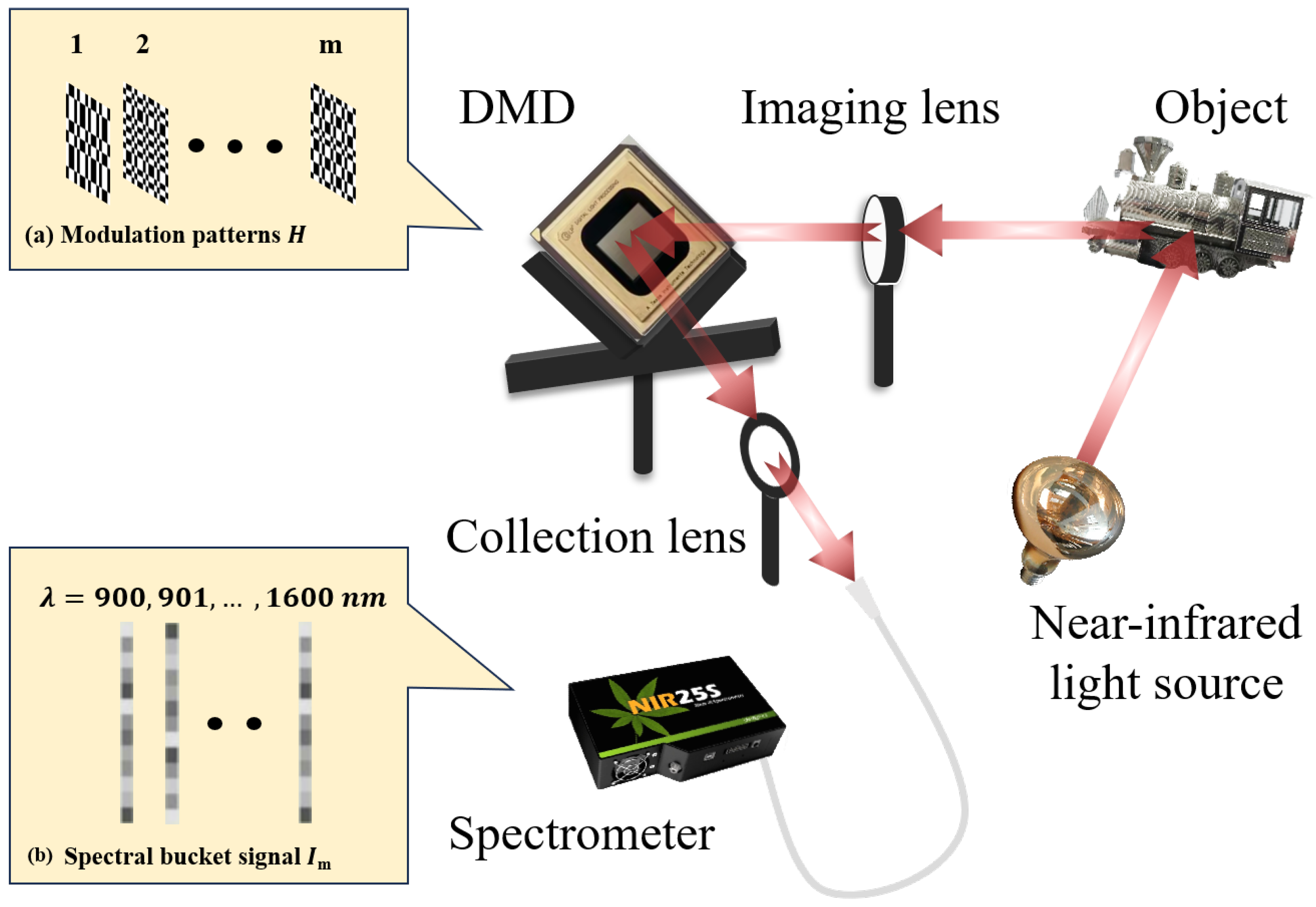
Figure 2.
The image reconstruction process by using the proposed physics-guided GAN method.

Figure 3.
The network structures of the proposed method, consisting of (a) the generator network and (b) the discriminator network.
Figure 3.
The network structures of the proposed method, consisting of (a) the generator network and (b) the discriminator network.

Figure 4.
Simulation test of the proposed method. (a1,a2) represent the ground truth images. (b1) shows the changes in the reconstruction quality of our method as the number of iterations increased. (b2) stands for the noisy image. (c1,d1) represent the changes in the generator and discriminator loss functions with the number of iterations. (c2–e2) represent the images recovered by the TVAL3 method, GIDC, and our method as the sampling rate (SR) increased, respectively.

Figure 5.
Results of reconstructing the physical train model using different methods. (a,b) represent the reconstruction results obtained using TVAL3, GIDC, and our method at SR = 20% and SR = 10%, respectively. From left to right, the wavelengths of light range from 880 nm to 1600 nm, with a step of 50 nm.

Figure 6.
Quantitative analysis results of single-pixel infrared HSI. (a) Two specific pixel locations were selected on the image, separately representing the reconstructed object part and the background part. (b,c) represent the results obtained at pixel ① and ② by three methods at different wavelengths. The black squares, red circles, and blue triangles stand for the TVAL3 method, GIDC method, and the proposed method, respectively.

Figure 7.
Comparisons of the efficiency and stability of different methods. (a,b) represent the results of the reconstructions at different iteration counts by our proposed method and the GIDC method, respectively.
Figure 7.
Comparisons of the efficiency and stability of different methods. (a,b) represent the results of the reconstructions at different iteration counts by our proposed method and the GIDC method, respectively.

Figure 8.
Comparisons of the impact of LRs on the results of image reconstruction. (a–d) represent the resulting images reconstructed by our proposed method at different LRs as the number of iterations increases.
Figure 8.
Comparisons of the impact of LRs on the results of image reconstruction. (a–d) represent the resulting images reconstructed by our proposed method at different LRs as the number of iterations increases.


Table 1.
Hardware configuration used in the experiment.
| Hardware | DMD (ViALUXV-2517001) |
| Imaging lens (f = 60 cm) | |
| Spectrometer (FUXIAN, NIR17+Px) |
Table 2.
Comparison of image reconstruction time using different methods at different SRs.
| SR = 10% | SR = 20% | |
| Ours | 51 s | 62 s |
| GIDC | 28 s | 36 s |
| TVAL3 | 6 s | 9 s |
Disclaimer/Publisher’s Note: The statements, opinions and data contained in all publications are solely those of the individual author(s) and contributor(s) and not of MDPI and/or the editor(s). MDPI and/or the editor(s) disclaim responsibility for any injury to people or property resulting from any ideas, methods, instructions or products referred to in the content. |
© 2024 by the authors. Licensee MDPI, Basel, Switzerland. This article is an open access article distributed under the terms and conditions of the Creative Commons Attribution (CC BY) license (https://creativecommons.org/licenses/by/4.0/).
Share and Cite
MDPI and ACS Style
Wang, D.-Y.; Bie, S.-H.; Chen, X.-H.; Yu, W.-K. Single-Pixel Infrared Hyperspectral Imaging via Physics-Guided Generative Adversarial Networks. Photonics 2024, 11, 174. https://doi.org/10.3390/photonics11020174
AMA Style
Wang D-Y, Bie S-H, Chen X-H, Yu W-K. Single-Pixel Infrared Hyperspectral Imaging via Physics-Guided Generative Adversarial Networks. Photonics. 2024; 11(2):174. https://doi.org/10.3390/photonics11020174
Chicago/Turabian StyleWang, Dong-Yin, Shu-Hang Bie, Xi-Hao Chen, and Wen-Kai Yu. 2024. "Single-Pixel Infrared Hyperspectral Imaging via Physics-Guided Generative Adversarial Networks" Photonics 11, no. 2: 174. https://doi.org/10.3390/photonics11020174
Note that from the first issue of 2016, this journal uses article numbers instead of page numbers. See further details here.