1. Introduction
Wireless laser communication has the advantages of high capacity, low latency, and high-throughput transmission. Its use in interplanetary channel application scenarios has been validated and has entered the engineering implementation stage [
1]. However, the use of airborne laser communication in airborne air-to-air channels involving turbulence has yet to be successfully applied due to the existence of many technical and engineering problems. Among these problems, the degradation of communication link quality or even the link’s interruption due to inter-symbol interference caused by the multipath effect is one of the most important problems affecting this technology’s reliability and availability [
2,
3]; it is also one of the key problems to be solved in airborne laser communication research.
Equalization is one of the techniques heavily used in the field of communication and is proven to be effective in mitigating or suppressing the effects of inter-symbol interference [
4,
5]. The goal of equalization is to make the communication system achieve as close to interference-free transmission conditions as possible using an equalizer (e.g., by restoring as much of the original transmitted signal waveform as possible after the detection of reception/before sampling judgment). Equalization is realized by eliminating as much inter-symbol interference as possible in the impulse response of the whole communication system, including the equalizer.
Channel technology is one of the most fundamental and crucial aspects in the field of wireless optical communication [
6]. Due to the typical time-varying and stochastic characteristics of the free-space channel, adaptive adjustments to the parameters of the airborne laser communication link equalizers are necessary to accommodate the dynamic nature of the channel.
Conducting research on the multipath transmission characteristics of on-board free-space laser channels is a prerequisite for studying equalization techniques in laser communication links. It forms the foundation for addressing issues related to inter-symbol interference, aiming to enhance communication quality and improve the reliability and availability of communication links.
The pulse broadening of laser beams after transmission through turbulent channels has been identified as the foremost factor contributing to inter-symbol interference in receiver systems. This paper employs the Monte Carlo ray tracing (MCRT) method to model and simulate the interactions of lasers with varying molecular and particle constituents within the turbulent atmospheres of free-space channels. The results of these simulations will yield the impulse response of the transmission channel, which is essential for supporting the design of equalizers [
7].
The objective of equalization is to realize interference-free transmission conditions in communication systems equipped with equalizers to the greatest extent possible. This involves restoring the original transmission signal waveform post-reception and pre-sampling/decision. The equalizer’s function is to ensure that the entire communication system, including the equalizer itself, satisfies the conditions for minimal inter-symbol interference. The channel’s impulse response obtained from simulations will guide and influence the overall design aspects of the equalizer, such as its structure, algorithm, convergence performance, and steady-state residual indicators. Due to the extensive nature of equalizer design considerations, these aspects will be discussed in a separate article.
In the present paper, a numerical MCRT simulation of airborne air-to-air channel laser multipath transmission and an analysis of inter-symbol interference is performed. The object of this analysis is to obtain the highest communication baud rate of a 2.5 Gbps airborne laser communication transmission link based on OOK (on-and-off keying) modulation, which is applied to an airborne air-to-air channel with an altitude of 10 km and a communication distance of 200 km (the meteorological conditions include the presence of high-altitude clouds and weak-to-moderate atmospheric turbulence intensity).
2. Airborne Air-to-Air Channel Laser Communication Link Analysis and Modeling
According to the information being transmitted from the source to the host of the transmission process, the airborne air-to-air channel laser communication link analysis model can be divided into four parts: laser emission, transmission, pupil reception, and detection and information processing, the specific process is shown in the
Figure 1.
A description of the constructed model is presented below:
At the transmitting end, the actual transmitting antenna aperture size is taken into account not only to constrain the size of the dispersion angle of the outgoing pupil beam but also to control the conditions of the outgoing beam ejection;
At the receiving end, taking into account the actual constraints on the field of view of the receiving antenna, one constraint of the simulated pupil reception process is that the transmission angle (stereo angle) of the photon transmitted to the receiving end’s face cannot be greater than the actual reception requirements of the receiving antenna’s field of view. A photon that fits within the constraints is considered a valid pupil reception photon and enters the subsequent photon counting process. Otherwise, the photon is invalid and does not enter the subsequent photon-counting process;
Considering the reception sensitivity power constraints of the actual system, a photon that is recognized as an effective pupil-received photon needs to meet both the low-limit power dimensions of the pupil and the constraints of the three-dimensional transmission angle of the pupil-received photon;
The actual ATP (acquisition, tracking, and pointing) error constraints in the airborne communication phase are considered.
The airborne ATP channel is a typical atmospheric turbulence channel and the refractive index structure constants of the turbulent channel under different altitude conditions can be described by the Hufnagel–Valley (H–V) correction model as follows [
3]:
In the above equation, is the altitude, whose unit is m, and represents the dimensions in .
The variance in the refractive index fluctuations, denoted as
, is a frequently employed physical parameter for characterizing atmospheric turbulence intensity. This dimensionless quantity exhibits a numerical order of magnitude comparable to the atmospheric refractive index structure constant
. Importantly, it is not contingent upon the assumption of turbulence isotropy, making it particularly well-suited for describing the intensity of atmospheric turbulence under general conditions. Here,
is the fluctuation in the refractive index at a single point;
has the unit m;
is the external scale of turbulence, whose unit is m; and
is the internal scale of turbulence, whose unit is m, which represents the distance between two points in space. According to Kolmogorov turbulence statistical theory, the structure–function
should be expressed as follows [
8,
9]:
3. Analytical Modeling of Pulse Time Broadening after Laser Transmission through Airborne Air-to-Air Channels
The total attenuation and effect of scattering on laser transmission in air-to-air laser communication links are affected by the working wavelength, transmission distance, and altitude of the cloud layer. Around the altitude of 10 km above sea level, laser transmissions in airborne air-to-air channel links will be affected by the scattering effects of various kinds of clouds. Clouds consist of tiny water droplets or ice crystals suspended in the air and their formation is mainly caused by the upward movement of moist air. The particle size, droplet content, and distribution of water droplets in various kinds of clouds and in clouds of varying thicknesses are not the same, which leads to differences in parameters such as the optical thickness of their scattering. Clouds vary greatly in height and thickness, with high-altitude clouds often being distributed in the 4.5 km–10 km region. The time–response characteristics of the laser pulse airborne channel transmission, obtained from the simulation of this transmission through clouds with different optical thicknesses, is an important input condition for the ISI simulation of the detection and reception phase.
Under meteorological cloud conditions, the airspace channel has random change characteristics and the clouds in the airborne air-to-air channel also present non-uniform distribution characteristics. The analysis of different parts of the cloud object is also relevant to determine the scattering and absorption characteristics of the different cloud types in order to more accurately describe the pulse-broadening characteristics of the laser beam transmitted through the channel and to provide a basis for the design of equalization programs. In this paper, an atmospheric scattering model and an atmospheric turbulence model are also established based on the airspace channel transmission time–response characteristics. Then, based on the atmospheric scattering model and atmospheric turbulence model, a Monte Carlo simulation model of the influence of the airborne air-to-air channel on the time-domain broadening characteristics of a Gaussian laser pulse is established. Combined with the design parameters of a typical airborne laser communication system, the Monte Carlo ray tracing (MCRT) method is used to simulate and analyze the time–response characteristics of the laser pulse through multiple cloud scattering channels.
The simulation modeling of laser multipath transmission through an airborne air-to-air channel focuses on the following two aspects [
10]: first, the Mie scattering effect generated by the interaction between the laser beam and the molecules and particles dispersed in the channel, and second, the change in the beam transmission direction due to the change in the atmospheric refractive index affecting the pulse time–response characteristics. The simulation model is shown in
Figure 2.
Airborne air-to-air channel laser transmission simulation modeling can be divided into the laser emission state setup, the laser cloud scattering transmission process (i.e., the generation of the free scattering range; the selection of scattering element parameters, Mie scattering effect, and scattering angle transformation; and the iterative simulation of continuous Mie scattering processes), the laser turbulence layer transmission process (i.e., laser and turbulence bulb interactions and iterative simulation of continuous turbulence effect process), and the identification of the effective pupil of the laser, in addition to other simulation and computation processes [
11,
12].
Taking the initial transmission coordinates as the origin, with the upward direction as the positive
x-axis and the leftward direction as the positive
y-axis, the transmission direction corresponds to the positive
z-axis. During laser transmission in the airborne air-to-air channel, the interaction between photons and the molecules and particles dispersed in the airborne transmission channel generates a number of consecutive Mie scattering effects, so that the transmission direction vector before and after each Mie scattering is
and
, respectively. The photon scattering angle is
in rad. The photon azimuth is
in rad and is described by a uniform distribution of random numbers in the range [0, 2π]. The iterative analytical model of the occurrence of continuous Mie scattering is as follows (a photon exiting the pupil into the null channel when the first Mie reflection occurs,
) [
13]:
In this formula, the mean free path between scattering events is denoted as , represents a uniformly distributed random number in the range [0, 1] and signifies the atmospheric attenuation coefficient.
Let
be a uniformly distributed random number in the range [0, 1]. The photon scattering angle
is then modeled as [
12]:
The analytical formula for the asymmetric factor
g is calculated as follows [
14]:
where
is the scattering element scale factor
; the asterisk (*) is the complex conjugate;
and
are the Mie scattering coefficients;
is the scattering element particle radius, whose unit is
; and
represents the wavelength, measured in
.
The relationship between the particle size and concentration of the scattering element can be characterized as obeying a lognormal distribution [
15]:
where
is the concentration of the particle in mode
i in
;
is the geometric mean particle size of the scattering element in
; and
is the geometric standard deviation of the scattering element in
.
The scattering element scattering efficiency
is calculated as follows [
15]:
The Mie scattering coefficient was chosen from the Bohren computational model below [
15].
where
is the complex refractive index of the scattering element;
is the scattering element scale factor,
;
is the radius of the scattering element; and
is the order of calculation of the Mie scattering coefficient, which is generally taken as
The scattering element absorption coefficient calculation model is given below as follows [
16]:
The modeling analysis of the pulse-broadening phenomenon resulting from the interaction between the photons transmitted via the airborne air-to-air channel and the turbulence is shown in
Figure 3.
In
Figure 3, the mean free path between turbulent bubbles, denoted as
, follows a Gaussian distribution with a mean of 1 m and a standard deviation of 0.9 m. Let
be a uniformly distributed random number in the range [0, 1]. The angle of incidence of a photon is
in rad and the angle of refraction of the photon is
in rad. The direction vector of the outgoing photon is
, the refractive index of the turbulent bulb is
, the reflectivity is
, and the refractive index is
(where
and
are the reflection coefficients of the
component and the
component).
From Fresnel’s equation, it follows that [
17]
Combined with Snell’s theorem, this gives [
18]
When
and
, the transmitted photon undergoes total reflection and the unit vector in the direction of the outgoing photon can be described by Equation (15). In this expression,
represents the unit vector in the photon incidence direction and
represents the unit vector in the direction normal to the photon incidence, satisfying
.
- 2.
When , refraction occurs between the transmitted photon and the turbulent bubble.
Let be the unit vector of the outgoing normal photon, ; let be the coordinates of the photon incident turbulence bubble point; let be the coordinates of the outgoing photon’s turbulence bubble point; let be the unit vector of the photon refracting direction; and let be the radius of the turbulence bubble.
The unit vector of the photon exit direction and the coordinates of the exit point under refractive conditions are calculated as follows:
To establish a free-space optical channel simulation model, this paper conducted laser transmission simulation research to achieve air-to-air airborne high-capacity communication. During the simulation process, typical parameters were employed for the developed equipment, along with meteorological parameters from a specific season in the Chengdu region, ensuring low optical beam pointing errors.
The specific parameters are as follows:
The parameters of the laser communication device used during the simulation are constrained to the following:
Operating wavelength, ; initial Gaussian pulse half-width, , with the transmitting and receiving antenna apertures being the same and ; exiting pupil divergence angle, ; entering pupil receiving field of view, ; beam alignment error angle, ; transmit power, ; receiver sensitivity, ; and transmission distance, , ;
The impact of scattering effects was modeled using the Mie scattering model;
The input parameters during the laminar transport simulation based on the photon/turbulence bubble model are as follows: standard deviation of atmospheric refractive index undulation, ; turbulence outer scale, ; and turbulence inner scale, ;
The atmospheric visibility of the airborne air-to-air channel was simulated by taking a set value of for all simulations, except for the unidirectional item simulation, which used different meteorological conditions.
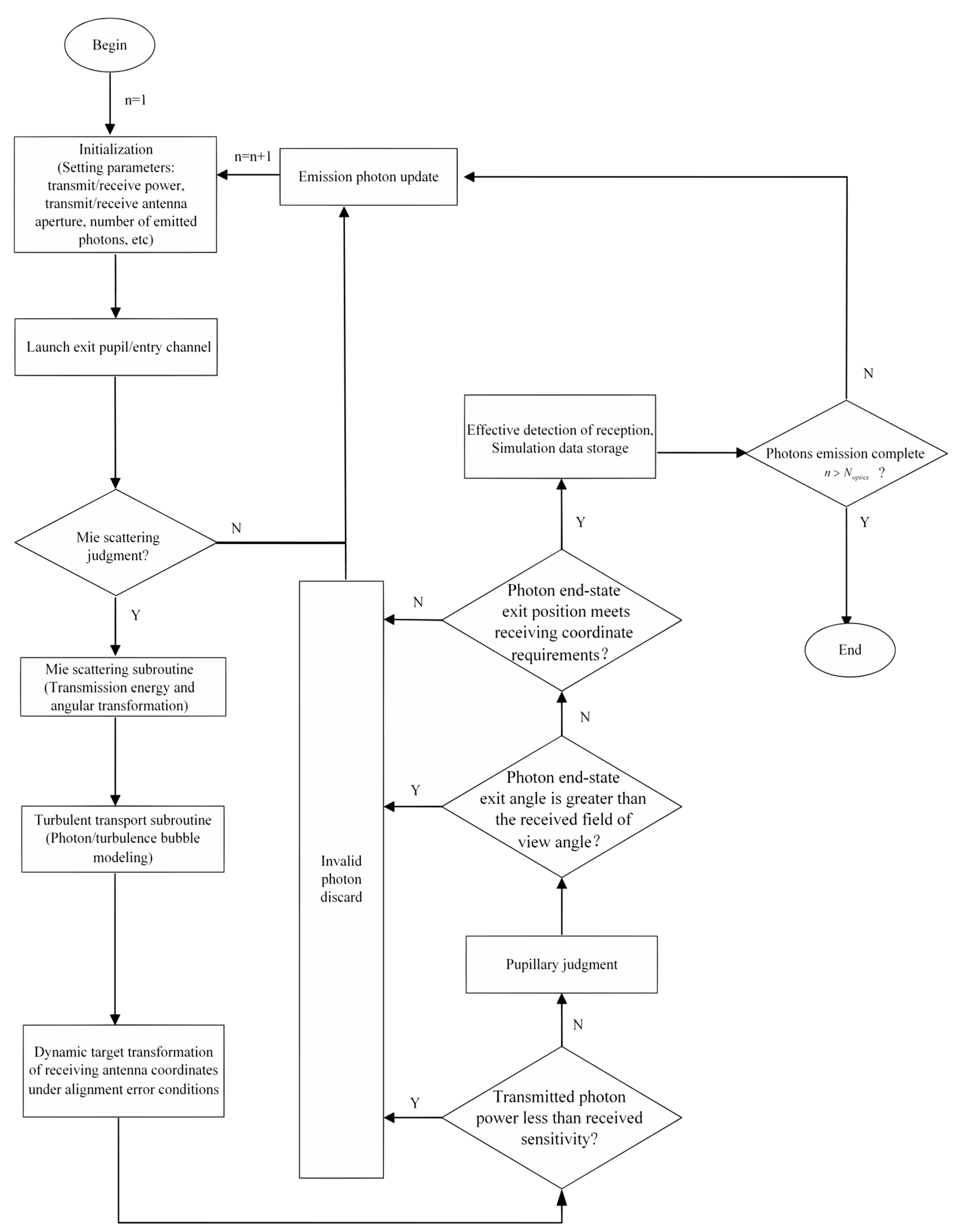
4. Laser Pulse Time–Response Characteristics Are Simulated and Analyzed under Different Influencing Factors and Change Conditions
The simulation will be divided into four parts, varying the turbulence intensity, atmospheric visibility, initial pulse half-width, and transmission distance for the simulation. The simulation flow is shown in
Figure 4.
In
Figure 4, n indicates that the current simulated photon is the nth photon and
is the total number of simulated photons.
The specific parameters of this simulation are shown in
Table 1.
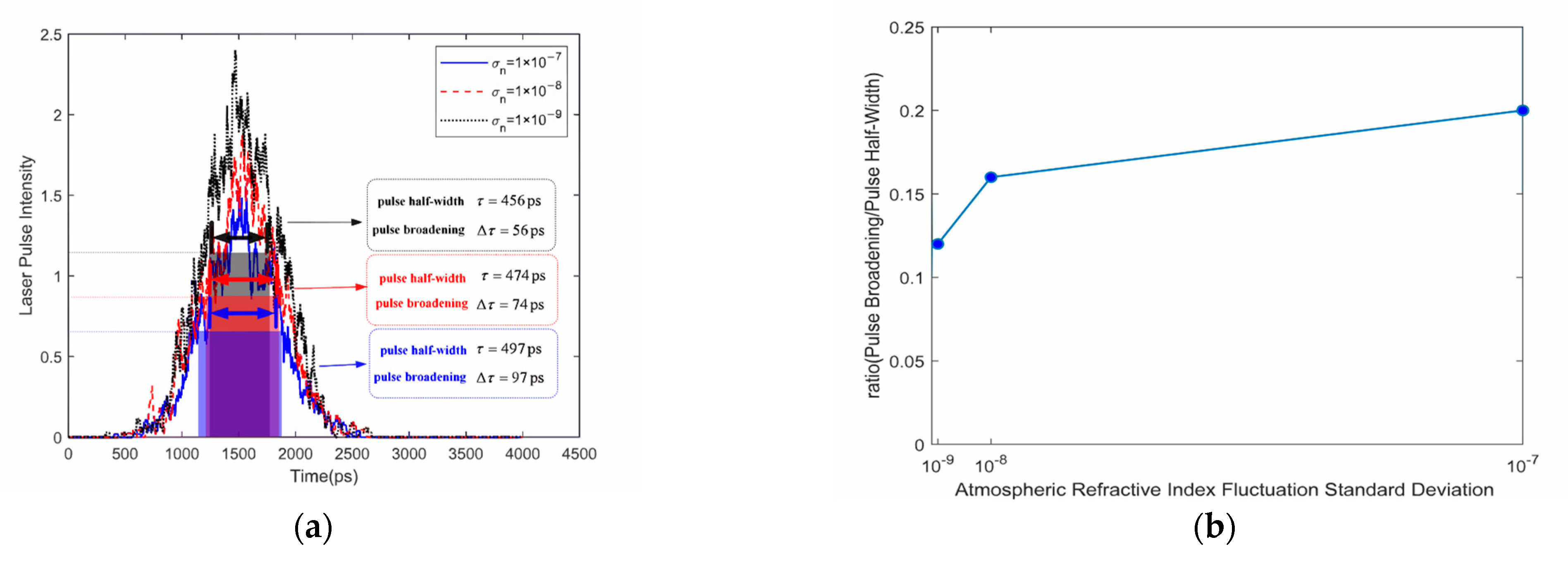
4.1. Simulation of Time–Response Characteristics of Laser Signals Transmitted through Airborne Air-to-Air Channels with Different Atmospheric Turbulence Intensities
In this subsection, the MCRT simulation of laser emissions after transmission over a multipath airspace channel with and without turbulence is carried out. The simulation results of the time-domain waveforms of the laser pulses after they are effectively received by the communication system (over a transmission distance of 200 km) are shown in
Figure 5a,b shows the laser pulse spreading and the half-width ratios of the laser pulses for the two transmission models considering different transmission distances. Mean and variance in laser pulse time-domain broadening for different transmission distances are shown in
Table 2.
Considering only the scattering effect without considering the effect of turbulence, the time-domain pulse broadening (pulse half-width) in ps after laser transmission is 22 (422) and the ratio of the laser pulse time-domain broadening to the pulse half-width is 5.2%. When considering the effects of scattering and turbulence at the same time, the laser time-domain pulse broadening (pulse half-width) is 74 (474) and the ratio of the laser pulse time-domain broadening to the pulse half-width is 15.8%. The simulation results show that the effect of the time-domain pulse broadening of the laser pulse due to turbulence effects in the airborne air-to-air channel is much larger than that caused by scattering effects.
Studies conducted at home and abroad [
19,
20,
21,
22] have shown that turbulence intensity generally decreases with height but that these changes are sporadic and the turbulence increases slightly at the top of the troposphere from 15 km to 18 km. Turbulence has a more obviously stratified structure with increasing height and because turbulence is intermittent in time and space, it is irregularly stratified, with stronger and weaker levels of turbulence throughout. The distribution of
, a structural parameter of the atmospheric refractive index, with altitude varies across different seasons in the same region as well as between day and night. In general, the turbulence intensity at high altitudes will be 1–2 orders of magnitude higher during the daytime than at night. In this paper, sounding test data on the daytime and nighttime turbulence of the airborne air-to-air channel collected at an altitude of 10 km over a region in the south of China in the summer [
21] were taken as the basis for analysis and inverse derivation was performed to obtain the standard deviation of the fluctuation in the atmospheric refractive index in the analyzed region. The
change in the study region is as follows:
,
. The analysis in this paper is based on clear weather scattering channel conditions and also simulates the time–response characteristics of laser signals transmitted via the airborne air-to-air channel under different standard deviations of fluctuation in the atmospheric refractive index and different turbulence channel conditions.
The standard deviations of the fluctuation in the atmospheric refractive index,
, are 97, 74, and 56 for the time-domain pulse spread and 497, 474, and 456 for the pulse half-width (in ps) of the airborne multipath channel in the presence of turbulence for the
, and
conditions, respectively. The simulation and analysis of time-domain waveforms of laser pulses with different standard deviations of atmospheric refractive index fluctuation are shown in
Figure 6. The ratios of the time-domain spread of the laser pulses to the pulse half-widths are 19.5%, 15.8%, and 12.3% for the three conditions, respectively. Mean and variance of in laser pulse time-domain broadening under different standard deviations of the fluctuation in atmospheric refractive index are shown in
Table 3.
The simulation results were analyzed and it was found that with the increase in the standard deviation of the fluctuation in the atmospheric refractive index, the time-domain spreading of the laser pulse caused by the airborne multipath channel is characterized by an increasing trend.
4.2. Simulation of Laser Transmission Characteristics under Different Visibility Conditions
In this paper, the time-domain waveforms of the laser pulse after transmission through multipath airborne channels with different visibility conditions are simulated using the MCRT method. The simulation results are shown in
Figure 7. As well as the mean and variance in laser pulse time-domain broadening under different atmospheric visibility conditions are shown in
Table 4.
The laser pulse broadening of the pulse signal time-domain and the pulse half-width (in ps) after transmission over 200 km is 98, 86, and 74 and 498, 486, and 474, respectively, for the airborne air-to-air channel under visibility conditions (in km) of 5, 20, and 50. The laser pulse time-domain spread to pulse half-width ratios are 20%, 18%, and 15.8%, respectively.
The analysis found that the laser beam is less influenced by the multipath effect when it is transmitted in an empty channel with greater visibility (i.e., a smaller number of molecules and particles dispersed in the channel) and that the time-domain spreading of the laser pulse after effective reception at the receiving end is smaller.
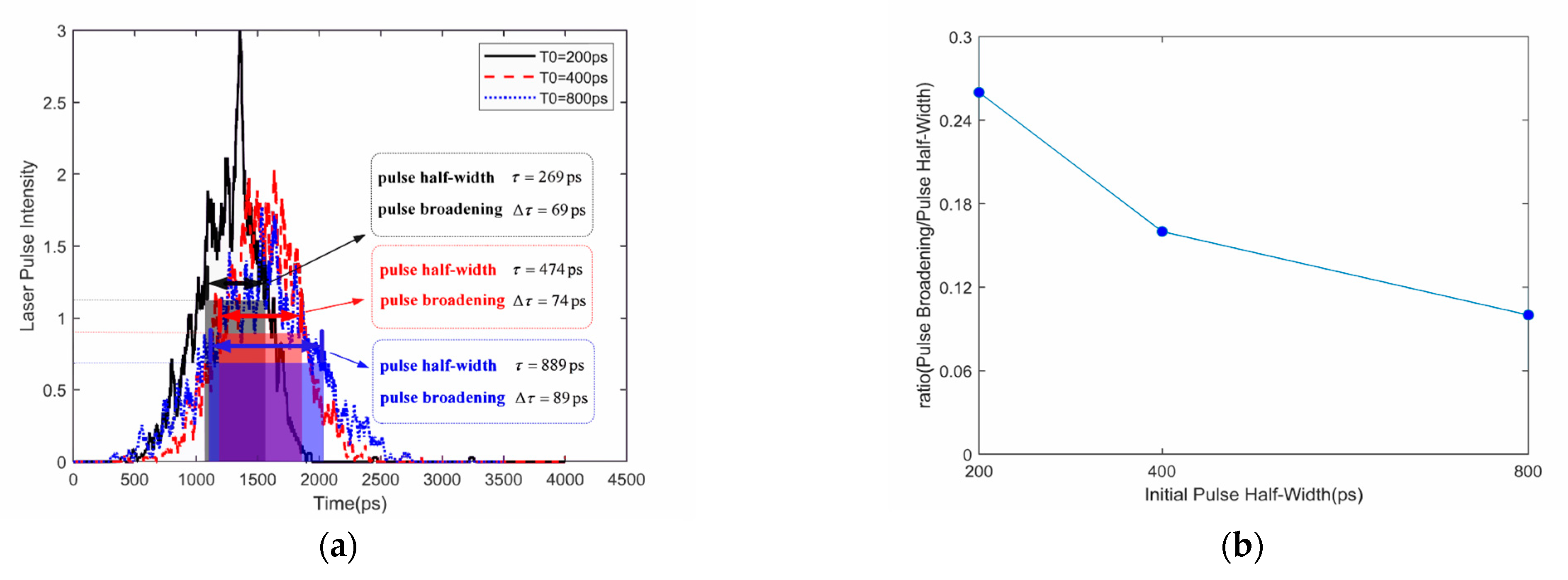
4.3. Simulation of Time–Response Characteristics after Laser Signal Transmission with Different Initial Pulse Widths
The time–response characteristics of laser signals after transmission with different initial pulse widths are simulated in the paper. The time–response characteristics of the laser pulse signal after transmission over a distance of 200 km corresponding to initial Gaussian pulse half-widths, in ps, of 200, 400, and 800 are shown in
Figure 8. The mean and variance in time-domain broadening of laser pulses under different initial pulse half-widths are shown in
Table 5.
Under the conditions in which scattering and turbulence are also considered, the corresponding pulse broadening (received pulse half-width) in ps of laser pulse signals transmitted through the airborne multipath channel with different initial pulse widths of 200, 400, and 800 ps are about 69 (269), 74 (474), and 89 (889). The ratios of the laser pulse time-domain broadening to the pulse half-width are 26%, 15.8%, and 10%, respectively. The simulation results of laser multipath transmission show that the percentage of laser pulse time-domain broadening caused by the airborne multipath channel tends to decrease with the increase in the initial pulse width of the transmitting laser.
4.4. Simulation of Laser Transmission Characteristics after Multipath Channel Transmission over Different Distances
The channel used for the simulation process features clear weather conditions and the laser time-domain pulse characteristics after air-to-air transmission over different distances (i.e., 150 km/200 km/250 km) are shown in
Figure 9. The mean value and variance in laser pulse time-domain broadening over different transmission distances are shown in
Table 6.
The laser pulse time-domain spread (pulse half-width) (in ps) after airborne transmission over different distances of 150 km, 200 km, and 250 km are 63 (463), 74 (474), and 85 (485), respectively. The laser pulse time-domain spread to pulse half-width ratios are 14%, 15.8%, and 18%, respectively.
An analysis of these results is presented below:
With the increase in transmission distance, the laser pulse transmitted by the airborne multipath channel will experience greater scattering and turbulence effects and within a certain range of the transmission distance, the time-domain broadening of the laser pulse effectively received by the antenna tends to increase;
With the increase in the transmission distance, the changing trend in the growth of the time-domain spread to pulse half-width ratio of the received laser pulse gradually stabilizes;
Considering the variation in the laser beam’s power density with the transmission distance, the number of pupil photons meeting the reception requirements will be reduced under the long transmission distances and the pulse broadening of the effectively received optical signal shows a gradual smoothing characteristic.
5. Detection of Received Signal Data Processing and ISI/BER Analysis
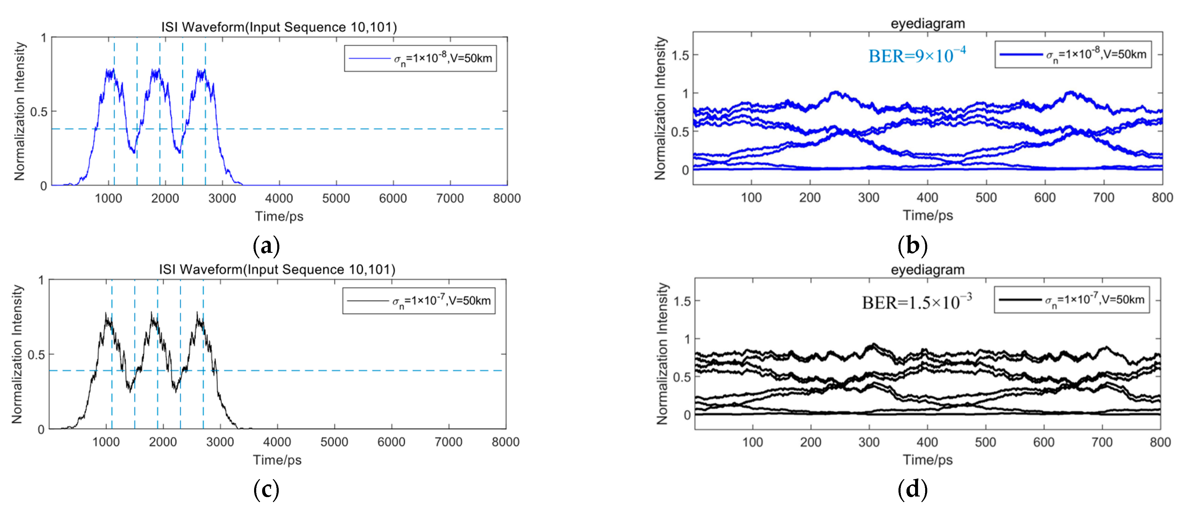
In this study, ISI simulation and BER statistical analysis of airborne laser communication links in the airborne air-to-air channel were conducted employing a 2.5 Gbps baud rate (OOK modulation). This was achieved by utilizing the established ISI analysis model and integrating the simulated channel impulse response derived from the air-to-air channel transmission simulation. Furthermore, the MATLAB simulation tool was employed to calculate and perform a comprehensive analysis of the bit error rate (BER).
Taking the results of the signal time–response curve obtained from the MCRT simulation as input parameters, combined with the design and development of the communication system, the simulation results show that the average single pulse spreading statistic is
when the standard deviation of the fluctuation in the atmospheric refractive index is
. The total pulse width statistic after sending 10,101 fixed code elements averages about 3000 ps and there is a certain ISI effect on the system (shown in
Figure 10a). This study modeled and simulated the changes in ISI in the front-end signal of the 2.5 Gbps airborne communication system’s receiving system based on OOK modulation.
The ISI waveforms of the received pulse signals, eye diagrams, and BER performance simulation results for the airborne channel with a visibility of
and different standard deviations of atmospheric refractive index fluctuation (
) are shown in
Figure 10. (Note: the transmitting codeword element is 10,101 and the number of BER statistical samples is 10,000).
The simulation results show that the average single pulse spreading statistic is
when the standard deviation of the fluctuation in the atmospheric refractive index is
. The total pulse width statistic after sending 10,101 fixed code elements averages about 3000 ps and there is a certain ISI effect on the system (shown in
Figure 10a). Moreover, the receiving eye diagram is slightly open, with a BER of
(shown in
Figure 10b). After the system implements equalization, anti-jamming coding, and other forms of technical processing to suppress inter-symbol interference, the quality of the communication link can reach the goal of high-performance communication.
When the standard deviation of the fluctuation in the atmospheric refractive index is
, the statistical average of a single pulse spread is
. The total pulse width statistics after sending 10,101 fixed code elements averages about 3000 ps and the system has a certain ISI influence (as shown in
Figure 10c). Moreover, the receiving eye diagram shows a microclosed state and the bit error rate is
(as shown in
Figure 10d). The system cannot establish a high-performance communication link under these conditions without using technical processing means such as equalization to suppress the inter-symbol interference.
The ISI waveforms of the received pulse signal and the simulation results of the eye diagram and BER performance for the airborne channel after transmission with a visibility of
and a standard deviation of the atmospheric refractive index fluctuation of
are shown in
Figure 11.
The simulation results show that the received pulse signal pulse spreading statistics after transmission over the airborne channel with a visibility of V = 20 km and standard deviation of atmospheric refractive index fluctuation averages . In addition, the total pulse width statistics after transmitting 10,101 fixed code elements averages about 3000 ps, with some evidence of ISI influence on the system; the receiving eye diagram shows a microclosed state and the bit error rate is BER = .
Combined with the simulation results in
Figure 10a,b, it can be seen that the laser pulse broadening after transmission via the air-to-air channel shows an inverse relationship with the channel’s visibility parameter: the higher the visibility, the smaller the pulse broadening.
The comparison of the phase and amplitude distortion corresponding to the time-domain pulse broadening extremes (maximum and minimum values) and the output waveforms under ideal conditions (without considering the effects of turbulence and absorption) under the typical operating conditions of airborne air-to-air channels is shown in
Figure 12.
An analysis of these results is presented below.
Under the simulation conditions of the thesis, the received time-domain pulse waveforms are all subject to different degrees of phase distortion after transmission over the airborne air-to-air channel. Among them, the received time-domain pulse signal with the most serious waveform distortion has a peak time shift of 1502.6 ns, which corresponds to a pulse spread of 98 ps, while the received time-domain pulse signal with a smaller waveform distortion has a peak time shift of 1502.0 ns, which corresponds to a pulse spread of 56 ps;
Under the simulation conditions of the thesis, the received time-domain pulse waveforms after transmission through the airborne air-to-air channel are subject to different degrees of amplitude distortion (manifested as a decrease in the peak amplitude). Compared with the peak value of the ideal received waveform, the maximum decrease in amplitude is (4.22 − 2.05)/4.22 = 51.42% and the minimum decrease in amplitude is (4.22 − 3.28)/4.22 = 22.27%.
The time-domain pulse waveform signal obtained after laser transmission through the airborne air-to-air channel reflects the channel’s characteristics. After the time-varying airborne air-to-air channel transmission with waveform distortion characteristics of the impulse response signal at the receiving end of the sampling process after the formation of the received signal sequence, the paper that analyzed airborne channel conditions combined with this paper on the airborne air-to-air channel laser transmission of the analysis of the time-domain pulse spreading results of the dual-mode (variable-step CMA + DDLMS) blind equalization scheme can be selected as one of the more reasonable equalization schemes. As shown in
Figure 13, the blind equalization scheme is one of the more reasonable equalization schemes.
The received sequence is processed by the transversal filter to form an output signal estimate , based on which the receiver decides that the output is the symbol of the transmitted message closest to as (defined as the desired response signal).
The error function is defined as and the size of the error function value can be used to guide the different equalization schemes actually adopted for subsequent data processing. When the dual-mode (variable step constant modulus algorithm (CMA) and direct decision least mean square (DDLMS)) blind equalization scheme is selected, the size of the error function value can be used as the judgment criterion for mode conversion and step transformation: when the error function value is large, it can be converted into the CMA blind equalization scheme with fast convergence speed (or increase the iteration step of the blind equalizer), and when the error function value is small, it can be converted into the DDLMS blind equalization scheme (or decrease the iteration step of the blind equalizer), which is characterized by a small steady-state error. When the error function value is small, it can be converted to the DDLMS blind equalization scheme with a small steady-state error (or reduce the iteration step size of the blind equalizer). The specific dual-mode blind equalization design scheme should also be based on the design principles of the overall scheme of the communication system and the actual application of the channel to determine the relevant content, described in another paper.


