1. Introduction
The adaptation of high-order modulation formats is regarded as one of the most effective schemes to improve both the spectral efficiency and the existing optical fiber infrastructure utilization efficiency [
1]. However, for a given optical transmission system, the highest achievable order of the modulation format is limited by its anti-noise performance and tolerance to linear and/or nonlinear transmission system impairments. Meanwhile, the optical network is required to meet heterogeneous and dynamic demands for supporting diverse data services, such as 5G, cloud computing, big data and the internet of things by optimizing the allocation of the bandwidth and modulation format. As a direct result, the optical network is evolving from fixed network architectures to flexible and elastic ones [
2,
3]. In elastic optical networks (EONs), according to different channel characteristics and various data services, the involved transceivers can dynamically adjust the modulation formats utilized for encoding the optical signals, which raises new demands on digital coherent receivers. Therefore, the MFI module embedded in a digital coherent receiver, which can identify the modulation format of incoming signals on-the-fly, is of great importance [
4]. MFI provides a foundation for optimizing the performance of subsequent modulation format-dependent algorithms in the digital signal processing (DSP) chain; as such, MFI is a critical technology to ensure the flexibility and reliability of the EON.
The previously reported MFI schemes for EON can be classified into data-aided and non-data-aided schemes [
5,
6,
7]. Since additional pilot information is introduced in the transmitter, the computational complexity of the data-aided schemes [
8,
9,
10] is thus low with an additional cost of a reduced spectral efficiency. On the other hand, without any special coding, the non-data-aided schemes can identify modulation formats based on the extracted features of the received signals. Non-data-aided schemes can be further roughly divided into schemes based on Stokes space and schemes based on the signal equalized by the constant modulus algorithm (CMA). Schemes based on Stokes space [
11,
12,
13,
14,
15,
16,
17,
18,
19,
20,
21,
22] are not sensitive to carrier phase noise, frequency offset or polarization mixing. However, it is difficult for these schemes to identify high-order modulation formats, which have a large number of clusters. On the flip side, the schemes based on CMA-equalized signals [
23,
24,
25,
26,
27,
28,
29,
30,
31,
32] do not require any space mapping, and CMA can partially compensate for residual chromatic dispersion (CD) and polarization mode dispersion (PMD) [
33,
34]. However, all of these schemes mentioned above are only suitable for identifying modulation formats up to 64QAM.
Generally speaking, the modulation format identification difficulty increases significantly upon increasing the modulation format order. To address this problem, an MFI scheme based on signal constellation diagrams and support vector machine (SVM) has been proposed in [
35], which identifies modulation formats up to 256QAM at the cost of computational complexity in the feature-extraction stage. The authors in [
36] have proposed an MFI scheme that utilizes a peak-density clustering algorithm to identify constellation diagrams of modulation formats up to 128QAM for adaptive optical OFDM systems. Zhang et al. [
37] have demonstrated a simultaneous MFI and OSNR monitoring scheme for QPSK, 8QAM, 16QAM, 32QAM, 64QAM and 128QAM signals based on multi-task model-agnostic meta-learning. An MFI scheme based on amplitude variance and OSNR information of the received signals has been proposed in [
38], which can identify modulation formats up to 2048QAM. However, the acceptable OSNR measurement error for this scheme is only ±0.2 dB.
In this paper, an MFI scheme based on multi-dimensional amplitude features is proposed for practical implementations in autonomous digital coherent receivers. In the proposed MFI scheme, after having performed power normalization, the numbers of CMA-equalized symbols in six specific amplitude ranges are calculated, based on which the six-dimensional feature of the incoming signals is constructed for the identification of different modulation formats. Since there are different amplitude levels for QPSK, 8QAM, 16QAM, 32QAM, 64QAM and 128QAM, the specific amplitude features of different modulation formats exhibit obviously different distributions in the six-dimensional space. Therefore, the multi-dimensional amplitude feature of the six modulation formats can be subsequently identified by KNN. The performance of the proposed MFI scheme is verified based on numerical simulations with 28GBaud PDM-QPSK/-8QAM/-16QAM/-32QAM/-64QAM/-128QAM signals. The results show that the proposed scheme can achieve 100% of the correct MFI rate for all of the six modulation formats when their corresponding OSNR values are higher than their theoretical 20% FEC limit. The simulation results also demonstrate that the proposed scheme is robust against both linear and nonlinear impairments. Finally, the computational complexity of the proposed scheme is analyzed. Our results indicate that the proposed technique can be regarded as a good candidate for identifying modulation formats up to 128QAM.
2. Operating Principle
As depicted in
Figure 1, the DSP chain for a digital coherent receiver consists of modulation-format-independent algorithms and modulation-format-dependent algorithms. The proposed MFI scheme is located between the modulation-format-independent algorithms and the modulation-format-dependent algorithms. Based on modulation-format-independent algorithms, the CD impairments and timing-jitters are compensated for, respectively, and the polarization demultiplexing is also preliminary achieved. Subsequently, the proposed MFI scheme is applied based on CMA-equalized signals and provides the information to the modulation-format-dependent algorithms (multi modulus algorithm (MMA), frequency offset compensation and carrier phase recovery) and symbol de-mapping.
As shown in
Figure 1, the proposed MFI scheme comprises three steps; firstly, power normalization of the CMA equalized signals is performed. Secondly, the amplitude histogram is obtained, which is then divided into six specific amplitude ranges. Finally, the numbers of symbols in the six specific amplitude ranges are calculated, based on which the six-dimensional feature of the incoming signals is constructed. The multi-dimensional amplitude feature of different modulation formats is subsequently identified by KNN.
The six modulation formats (QPSK, 8QAM, 16QAM, 32QAM, 64QAM and 128QAM) have different amplitude levels and are theoretically easy to identify. However, under the influence of the channel noise, residual CD, PMD and fiber nonlinearities, the amplitude features of the received signals in practical transmission systems are difficult to recognize, especially for high-order modulation formats. The amplitude histograms of these six modulation formats are illustrated in
Figure 2, where the OSNR values for the PDM-QPSK/-8QAM/-16QAM/-32QAM/-64QAM/-128QAM signals are 26 dB, 31 dB, 33 dB, 36 dB, 38 dB and 40 dB, respectively. The amplitude histograms shown in
Figure 2 are obtained utilizing 8000 symbols, which are grouped into 40 bins between the maximum and minimum amplitude values of the CMA-equalized signals. As shown in
Figure 2, even for high OSNR cases, the different amplitude levels of high-order modulation formats cannot be easily distinguishable. Therefore, relying solely on the global feature of the amplitude histogram cannot identify signal modulation formats higher than for 128QAM.
To address such a challenge, the scheme proposed in this paper adopts a more efficient local feature extraction approach. As illustrated in
Figure 2, the numbers (
N1,
N2,
N3,
N4,
N5 and
N6) of the CMA-equalized symbols in six specific amplitude ranges (
A1~B1, A2~B2,
A3~B3,
A4~B4,
A5~B5 and
A6~B6) are utilized to construct six-dimensional features of the incoming signals. As shown in
Figure 2a, due to the constant amplitude of QPSK, as noise or other transmission impairments gives rise to few symbols deviated from the constant amplitude, the number of symbols within the range from
A1 to
B1 is thus very small. Therefore,
N1 within the range of
A1~B1 can be employed to separate QPSK from the other five modulation formats. For the same reason, as shown in
Figure 2b,
N2 for the range of (
A2~B2) (the number of symbols distributed in the second half of the first amplitude peak of 8QAM) can be used as a feature for identifying 8QAM. Similarly,
N3 and
N4, representing the numbers of the symbols distributed in the first half of the first amplitude peak of 16QAM, (
A3~B3), and the first half of the first amplitude peak of 32QAM, (
A4~B4), can be employed as distinct features for identifying 16QAM and 32QAM, respectively. Although there are nine amplitude levels for 64QAM, its corresponding amplitude histogram does not, however, clearly illustrate nine distinguishable levels in the presence of noise. Since the associated probability for the sixth amplitude level of 64QAM is highest [
3],
N5, representing the number of symbols within the range of (
A5~B5), can thus be calculated to extract the feature for 64QAM.
N1,
N2,
N3,
N4 and
N5 mainly represent the features located in the front and middle of the relevant histograms, whilst
N6 for 128QAM extracts the feature located in the last part of the histogram. 128QAM exhibits different distributions within the range of (
A6~B6). The ranges
A1~
B1,
A2~
B2,
A3~
B3,
A4~
B4,
A5~
B5 and
A6~
B6 are 1~16, 14~22, 4~12, 1~8, 25~28 and 34~40, respectively. It should be noted that the identification performance is dependent on the effectiveness and irreplaceability of features rather than dimensions of the feature. Excessive features would lead to confusion among different modulation formats in the multi-dimensional space, and thus, only six dimensional features are selected.
Due to the noise effect, even the features of the same modulation format may appear to be different for different OSNR conditions, but the distribution of the different modulation formats in the six-dimensional space is still sharply distinguishable. In order to verify the above statement,
Figure 3 is plotted, where the features in a three-dimensional space are shown by using three of the six features as coordinates (
N1,
N2,
N4 for
Figure 3a–c,
N1,
N5,
N6 for
Figure 3d and
N1,
N3,
N4 for
Figure 3e,f). The distribution of the six modulation formats in the three-dimensional space based on
N1,
N2 and
N4 is illustrated in
Figure 3a. Two different views of
Figure 3a from two different angles are given for (QPSK, 8QAM, 16QAM) in
Figure 3b and (32QAM, 64QAM,128QAM) in
Figure 3c. From
Figure 3a,b, it can be clearly seen that QPSK and 8QAM can be easily distinguished from the other four modulation formats. Meanwhile, 32QAM, 64QAM and 128QAM are also distinguishable among each other. As shown in
Figure 3a, 16QAM is not distinguishable from 32QAM, 64QAM and 128QAM in the three-dimensional space (
N1,
N2 and
N4). However, as shown in
Figure 3d–f, 16QAM can be distinguished easily from 32QAM, 64QAM and 128QAM based on the other three features (
N1,
N5 and
N6 for separating 32QAM, and
N1,
N3 and
N4 for separating 64QAM or 128QAM), respectively. The above analysis indicates that when the six-dimensional features are regarded as a whole, the six modulation formats can be identified.
KNN is an effective supervised learning algorithm commonly used in classification problems. As shown in
Figure 3, the modulation format of an incoming signal can be easily determined by nearby training samples in the six-dimensional space. Compared with another classification algorithm SVM, which makes decisions based on hyperplanes, KNN is more suitable for identifying the extracted features. Therefore, as depicted in
Figure 4, KNN is employed to recognize the six-dimensional features (
N1,
N2,
N3,
N4,
N5 and
N6). The Euclidean distance
d between a test sample and each training sample in the six dimensional space is calculated as
where
x1j denotes the
j-th feature of the test sample, and
x2j represents the
j-th feature of the training sample. According to the size of the
k value, the KNN finds
k training samples in the training dataset that are closest to the test sample, and then, for a randomly given category
i, the number of occurrences of the category in the
k nearest training samples is known. Finally, as shown in Equation (2), the category of the test sample is determined based on the category with the most occurrences among the
k nearest training samples.
where
V is the occurrences among the
k nearest training samples for category
i, and
i* is the determined category for the test sample. Since the input of KNN is only six-dimensional, the extracted local amplitude feature not only represents the characteristic of modulation format, but also significantly reduces the complexity of KNN compared to the global feature.
3. Results and Analysis
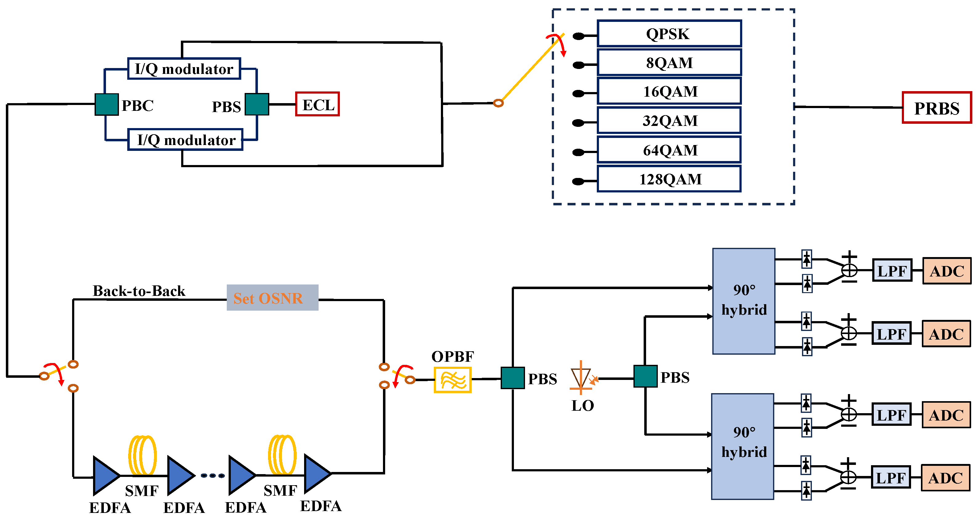
To verify the proposed scheme, a series of numerical simulations is conducted based on
VPI Transmission Maker 9.8. The simulation setup of a PDM coherent optical transmission system is illustrated in
Figure 5. In all of the simulations, external cavity laser (ECL) is operated with 100 kHz linewidths. Six modulation format (QPSK, 8QAM, 16QAM, 32QAM, 64QAM and 128QAM)-encoded optical signals are generated by driving the I/Q modulator with a binary 28Gbaud electrical signal. The transmission links comprise back-to-back (BTB) and long-distance fiber transmissions. The OSNR value of the BTB case is adjusted by the Set OSNR module. The OSNR ranges of the PDM-QPSK/-8QAM/-16QAM/-32QAM/-64QAM/-128QAM-encoded signals are 5~24 dB, 10~29 dB, 12~31 dB, 16~35 dB, 17~36 dB and 23–42 dB, respectively. The long-distance transmission link is composed of
M × 80 km (
M = 25 for QPSK,
M = 20 for 8QAM,
M = 13 for 16QAM,
M = 5 for 32QAM,
M = 2 for 64QAM,
M = 1 for 128QAM) spans of single-mode fibers (SMFs) that have a dispersion parameter of
D = 16 ps/nm/km, a PMD parameter of
DPMD = 0.1 ps/km
1/2, an attenuation of
α = 0.2 dB/km and a nonlinear coefficient of
γ = 1.267 km
−1W
−1. The fiber loss of each span is completely compensated for per span using an erbium-doped fiber amplifier (EDFA) with a noise figure of 5 dB. At the receiving end, the incoming signals and the local oscillator (LO) are combined at a polarization diversity hybrid, and then, the photo is detected by a balanced photo-detector. Then, the digital signals that have been sampled by an analog to digital converter (ADC) are processed by an off-line DSP module. A training set is constructed by using eighty samples for each OSNR value and each modulation format in the BTB case, and the training set is then applied for both BTB and long-distance testing. Twenty samples are applied to validate a correct MFI rate for each OSNR value in the BTB case or for each launch power in the long-distance transmission case.
The minimum required number of symbols determines the response-speed and computational complexity of the MFI algorithm [
26]; on the other hand, too few symbols would result in a fuzzy feature, especially for high-order modulation formats. The minimum required OSNR values for the six modulation formats as a function of the number of symbols are shown in
Figure 6a,b, and the step sizes are 1000 and 250, respectively. If the number of symbols is less than 7000, for most of these modulation formats, the minimum required OSNR values to achieve a 100% correct MFI rate increase accordingly. On the other hand, 128QAM requires more symbols to accurately extract the feature. In order to find the optimal number of symbols, the step size of the symbol number is decreased to 250 in
Figure 6b. Although the minimum required OSNR value for 128QAM is optimal when the number of symbols is 7500, the minimum required OSNR values for 8QAM, 16QAM, 32QAM and 64QAM are, however, greater than these for the 8000 symbols case. Considering the tradeoff between all the six modulation formats, the required numbers of symbols for the six modulation formats are thus fixed at 8000.
As analyzed in
Section 2, the KNN determines the modulation format of an incoming signal based on the categories of the
k nearest training samples. The value of
k is an important parameter and determines the identification performance of KNN. Similar to the process used in
Figure 6, an optimal
k value should also be identified with the minimum required OSNR value. The simulated results are illustrated in
Figure 7. When the value of
k increases from 1 to 9, the minimum required OSNR values for QPSK, 8QAM and 64QAM remain unchanged, while the minimum required OSNR values for 16QAM and 32QAM increase slightly. It can also be clearly seen in
Figure 7 that the optimal
k value for 128QAM is 3. Therefore, for all of the considered modulation formats, the
k value is taken to be 3.
To evaluate the identification performance of the proposed scheme, the correct MFI rate for each individual modulation format as a function of OSNR is shown in
Figure 8. The vertical dash lines are the OSNR thresholds corresponding to the 20% FEC related to BERs of
. For QPSK, 8QAM, 16QAM, 32QAM and 64QAM, the proposed MFI scheme can achieve 100% of the correct MFI rate even if the OSNR value is much less than the corresponding theoretical 20% FEC limit. Since 128QAM is the highest order of the six modulation formats, the minimum required OSNR for 128QAM is much higher than the other five modulation formats.
Figure 8 indicates that the proposed MFI scheme can achieve 100% of the correct MFI rate for all six modulation formats when the OSNR values are greater than their corresponding thresholds related to the 20% FEC.
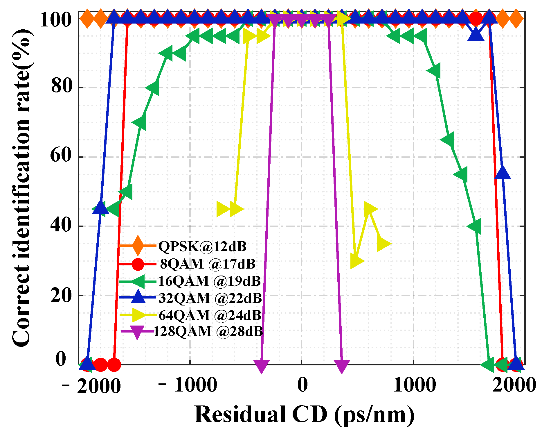
In order to evaluate the effect of the residual CD on the MFI performance, numerical simulations have also been conducted under conditions of the OSNR values of QPSK, 8QAM, 16QAM, 32QAM, 64QAM and 128QAM being set at 12 dB, 17 dB, 19 dB, 22 dB, 24 dB and 28 dB, respectively. In addition, the range of the residual CD for QPSK, 8QAM, 16QAM and 32QAM signals is −1920 ps/nm~1920 ps/nm, while the ranges of the residual CD for 64QAM and 128QAM signals are −720 ps/nm~720 ps/nm and −360 ps/nm~360 ps/nm, respectively. The step sizes for the six modulation formats are both 120 ps/nm. As illustrated in
Figure 9, the proposed MFI scheme can tolerate wide ranges of residual CD, i.e., −1920 ps/nm~1920 ps/nm for QPSK signals, −1560 ps/nm~1680 ps/nm for 8QAM signals and −1680 ps/nm~1440 ps/nm for 32QAM signals. The identification accuracy of 16QAM is still maintained at >95% over a wide residual CD range, while the tolerance with respect to the residual CD for 16QAM is only −480 ps/nm~720 ps/nm. Because of the existence of more amplitude levels for 64QAM and 128QAM, the sensitivity of the extracted features against residual CD is much greater than low-order modulation formats, and thus, the tolerances with respect to residual CD for 64QAM and 128QAM are much lower (−240 ps/nm~360 ps/nm for 64QAM, and −240 ps/nm~240 ps/nm for 128QAM).
Simulations have also been undertaken to evaluate the effect of PMD on the MFI performance, and the simulated results are shown in
Figure 10, in simulating which the range of differential-group delay (DGD) for QPSK, 8QAM, 16QAM and 32QAM signals is taken from 0 ps to 34 ps with a step size of 2 ps, while the range of DGD for 64QAM signals is taken from 0 ps to 22 ps with a step size of 2 ps. As shown in
Figure 10a, the proposed scheme is able to achieve 100% of the correct MFI rate for the QPSK, 8QAM, 16QAM, 32QAM and 64QAM signals even when the DGDs are 34 ps, 32 ps, 16 ps, 20 ps and 10 ps, respectively. Compared to the aforementioned modulation formats, since 128QAM’s DGD tolerance is significantly decreased, the range of DGD for 128QAM signals is from 0 ps to 2.4 ps with a step size of 0.2 ps. The tolerable DGD range for 128QAM signals is 1.6 ps, which is much lower than the other five modulation formats.
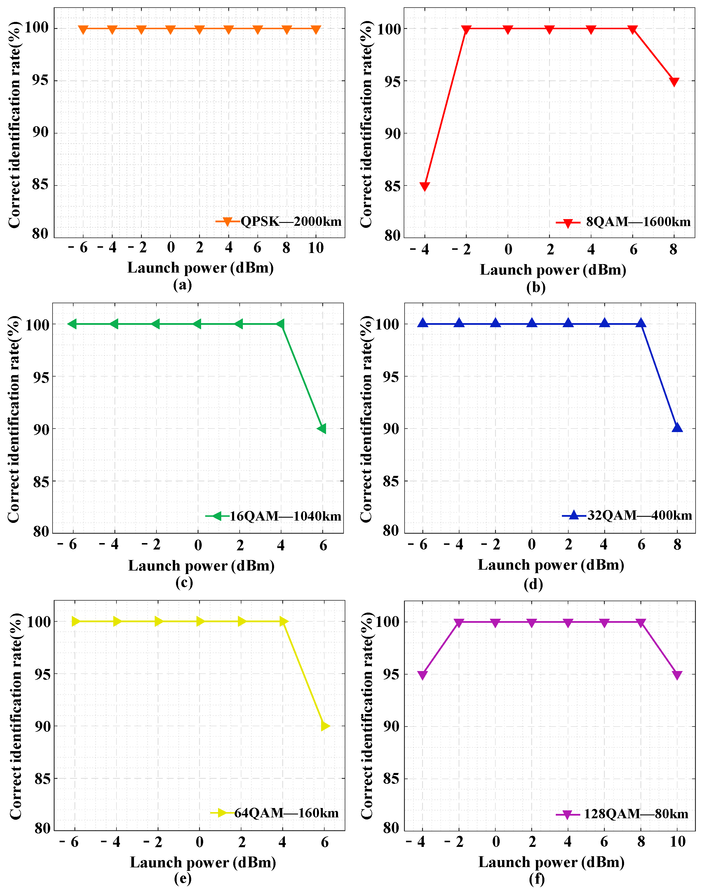
In order to analyze the effect of nonlinear impairments, a series of long-distance transmission simulations for QPSK (2000 km), 8QAM (1600 km), 16QAM (1040 km), 32QAM (400 km), 64QAM (160 km) and 128QAM (80 km) signals is conducted. The correct MFI rates of the six modulation formats versus the launch power in long-distance transmissions are shown in
Figure 11. The proposed scheme can achieve 100% of the correct MFI rate even when the launch powers are increased to 10 dBm, 6 dBm, 4 dBm, 6 dBm, 4 dBm and 8 dBm for QPSK, 8QAM, 16QAM, 32QAM, 64QAM and 128QAM signals, respectively. These results demonstrate that the proposed MFI scheme is robust against fiber nonlinearities.
Finally, to comprehensively evaluate the performance of the proposed scheme with respect to other relevant MFI schemes based on deep neural network (DNN) [
39] and SVM, their performance comparisons are made in
Figure 12, where the number of symbols and histogram bins are fixed at 8000 and 40, respectively. The training sets for DNN and SVM comprise 9600 (20 × 80 × 6) amplitude histogram samples. For DNN, the numbers of neurons in the input, first hidden, second hidden and output layers are 40, 40, 10 and 6, respectively. The activation functions of the hidden layer and output layer are
ReLU and
softmax, respectively [
40]. For SVM, the kernel function is the default radial basis function (RBF) kernel [
41].
Based on the simulation results for both DNN and SVM, the minimum required OSNR comparisons between the proposed scheme and these two schemes based on DNN and SVM are shown in
Figure 12. For QPSK, 8QAM, 16QAM, 32QAM and 64QAM, the minimum OSNR values required for achieving 100% of the correct MFI rate for the proposed scheme are lower than or equal to those corresponding to schemes based on DNN and SVM. Most importantly, only the proposed scheme can identify 128QAM over a wide OSNR range. Unlike the proposed scheme, the DNN and SVM just identify the global feature of the amplitude histogram. Since the characteristics of modulation formats are not effectively extracted based on the global feature of the amplitude histogram only, the MFI schemes based on DNN and SVM cannot identify 128QAM.
To evaluate the computational complexity of the proposed scheme, the execution times for the three MFI schemes are analyzed. All of KNN, DNN and SVM are implemented by
MATLAB R2021a, which run on a conventional computer equipped with a Core i7-10700 CPU at 2.9 GHz and 16 GB RAM. The graphics card is RTX2060 with 12 GB of memory. Unlike DNN and SVM, KNN does not require any training process. However, it should be noted that the training set for KNN needs to be introduced into
MATLAB R2021a. The time of data input is 0.18 s, which is much less than the time used for the training of DNN and SVM, as shown in
Figure 13a. Since the dimension of the extracted feature for the proposed scheme is only six, which is much less than the dimension of the amplitude histogram, the complexity of KNN is thus significantly reduced. The times used for the prediction of each testing sample in the three MFI schemes are depicted in
Figure 13b. The time used for the prediction of the proposed scheme is also much less than those corresponding to the MFI schemes based on DNN and SVM. Therefore, the computational complexity of the proposed scheme is competitive.

 ,
, 