Low-Cost High-Speed Fiber-Coupled Interferometer for Precise Surface Profilometry


Abstract
:1. Introduction
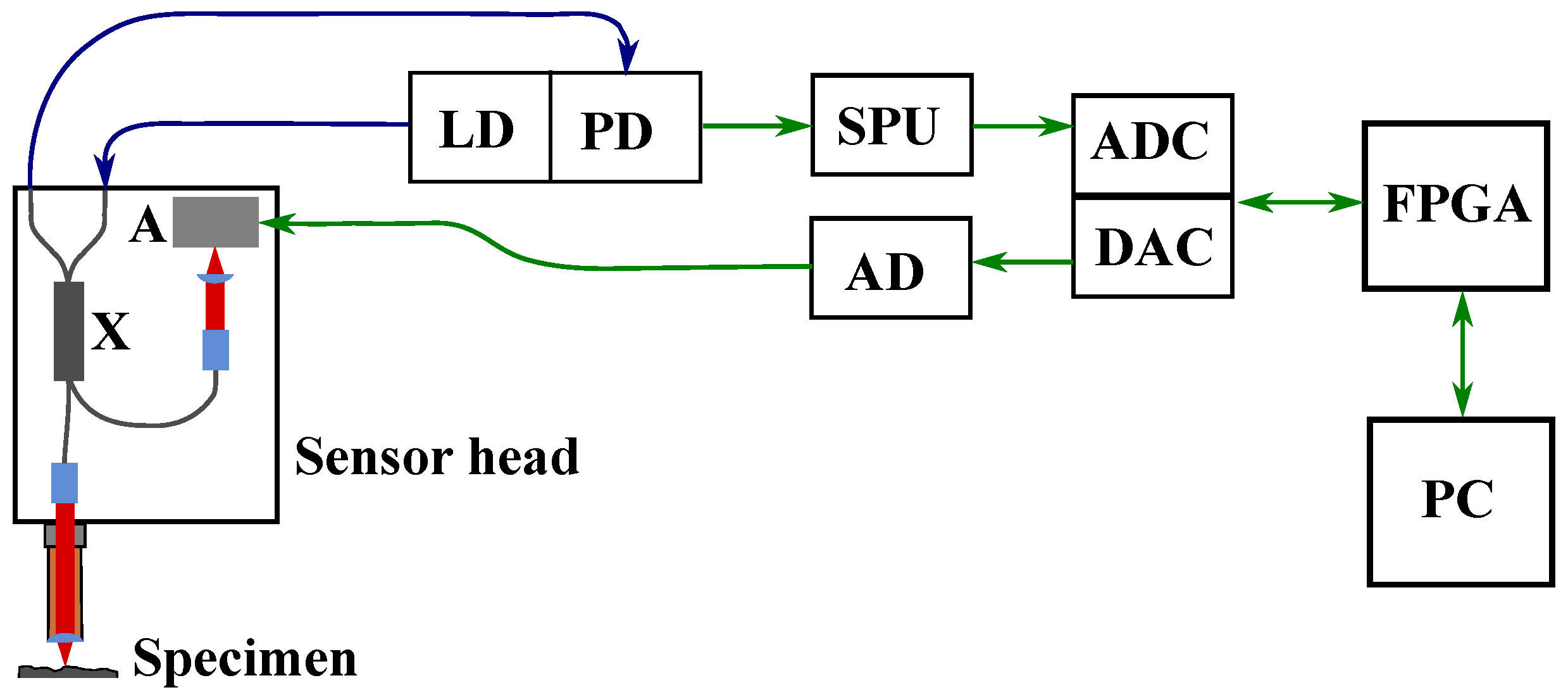
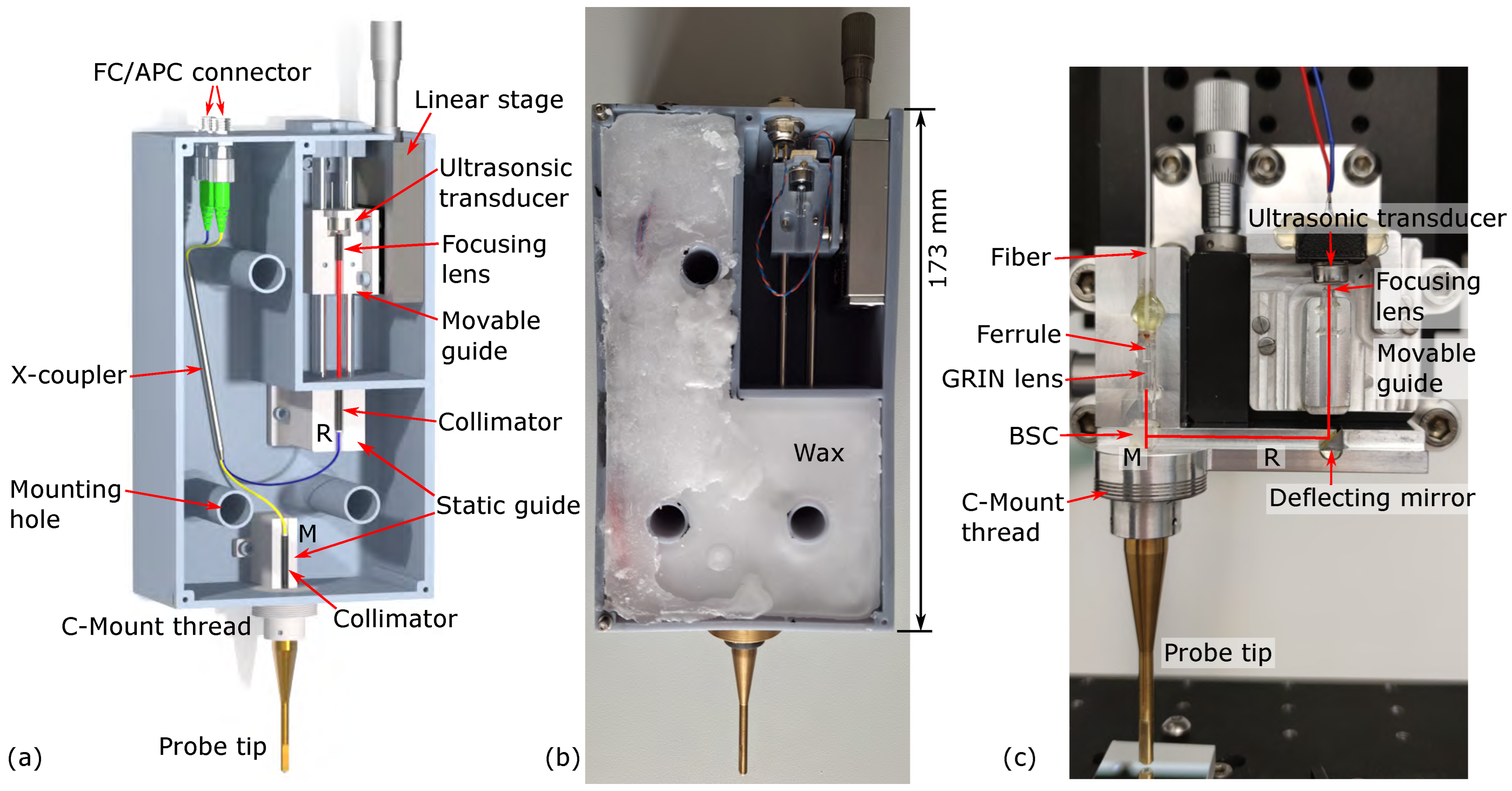
2. Sensor Setup
2.1. Interferometric Sensor
2.2. Signal Processing
3. Results
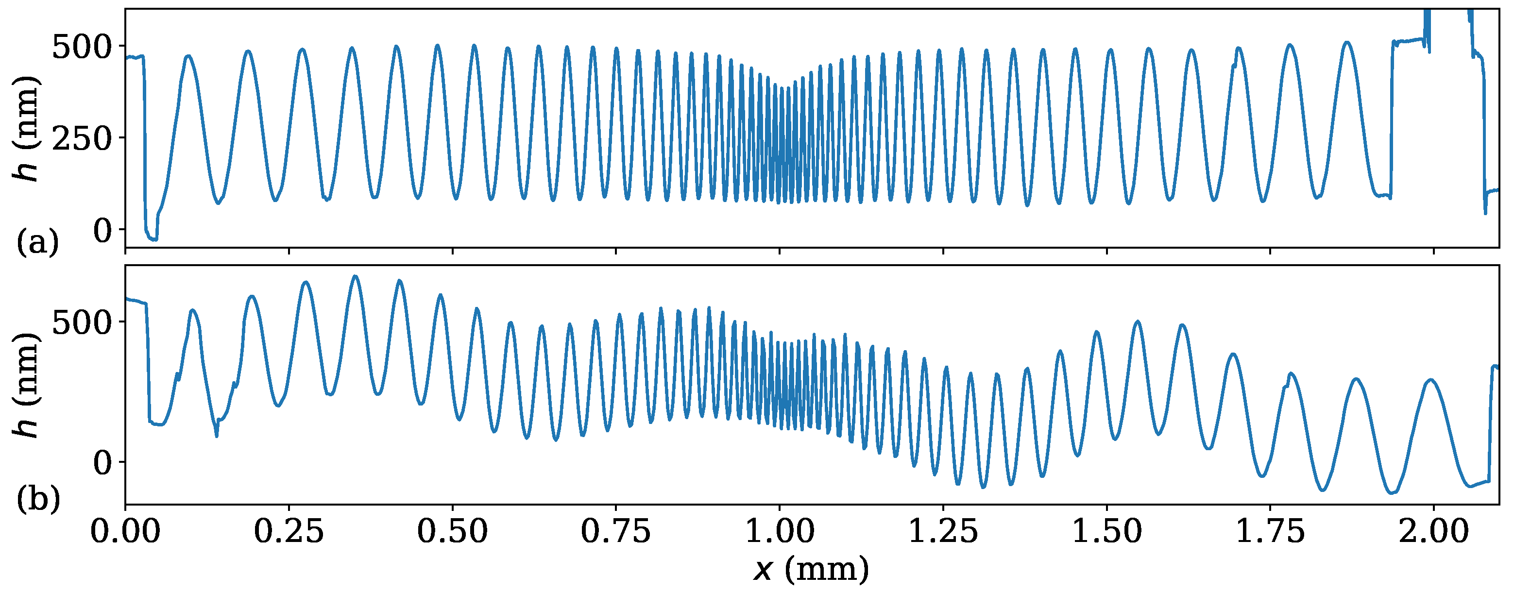
3.1. Chirp Standard
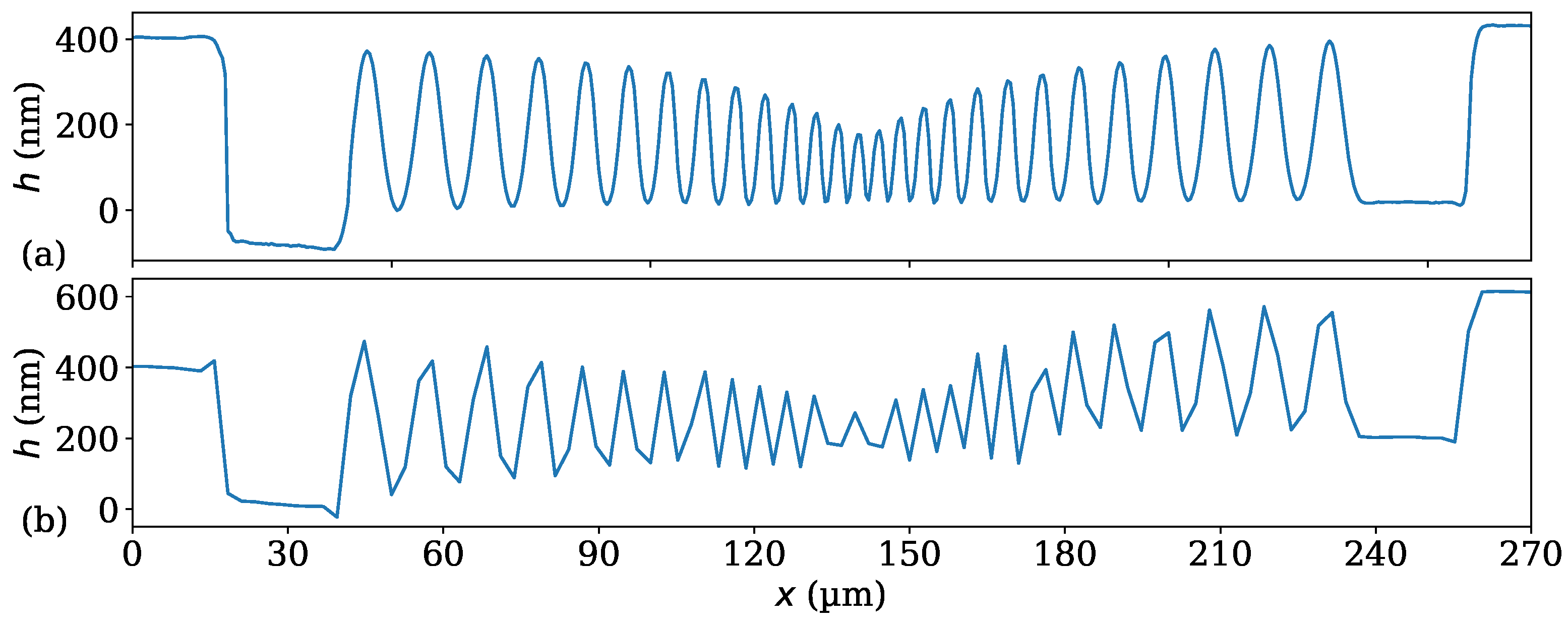
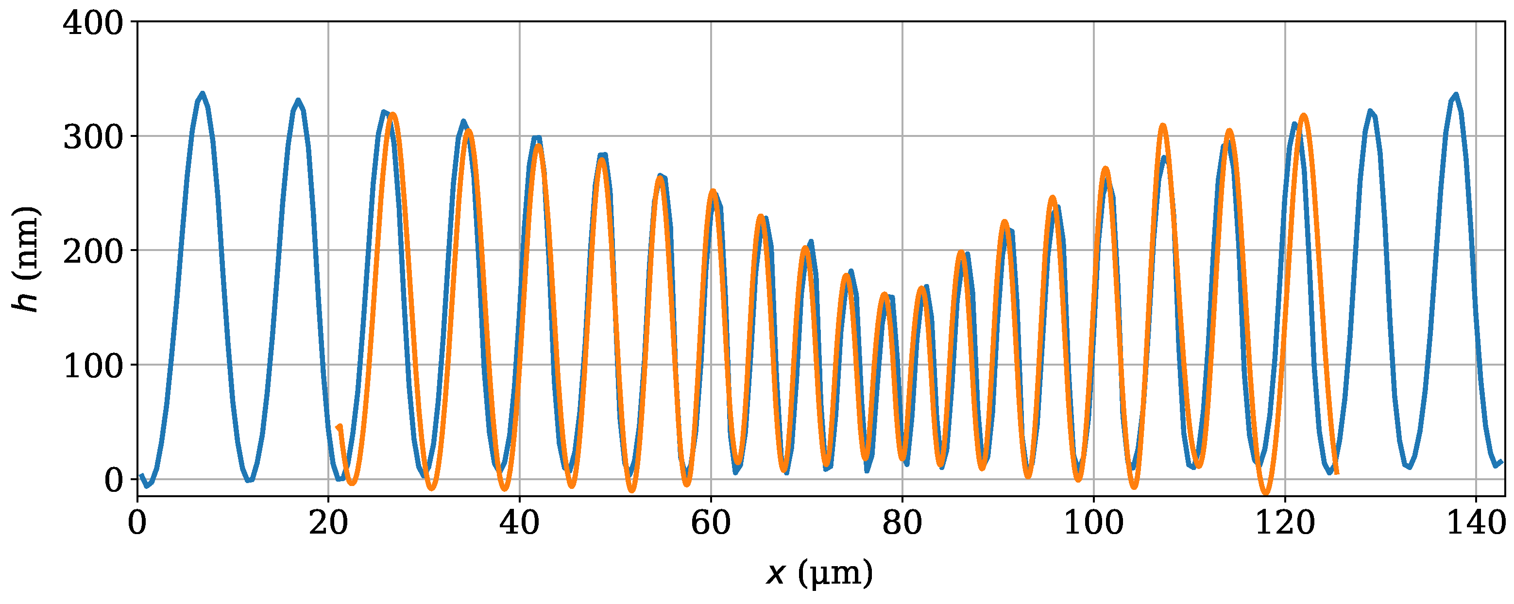
3.2. Sinusoidal Standard
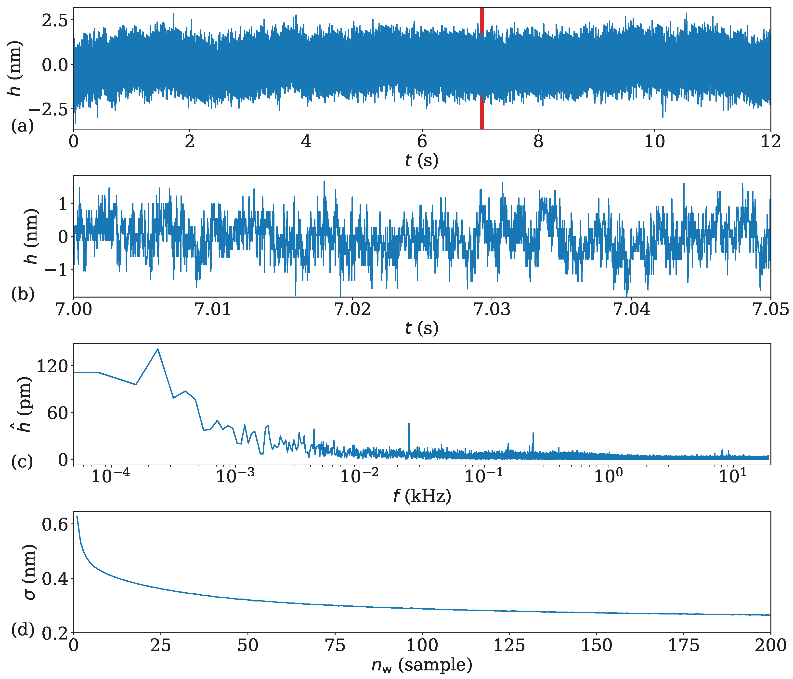
3.3. Repeatability
4. Conclusions
Author Contributions
Funding
Institutional Review Board Statement
Informed Consent Statement
Data Availability Statement
Conflicts of Interest
Abbreviations
| A | Actuator |
| AD | Actor driver |
| ADC | Analog-to-digital converter |
| AFM | Atomic force microscopy |
| APC | Angled physical contact |
| BSC | Beam-splitter cube |
| DAC | Digital-to-analog converter |
| FC | Ferrule connector |
| FICDS | Fiber-coupled interferometric confocal distance sensor |
| FPGA | Field programmable gate array |
| HMSC | High-speed mezzanine card |
| LD | Laser driver |
| M | Measurement arm |
| NA | Numerical aperture |
| OPD | Optical path-length difference |
| PC | Personal computer |
| PD | Photodiode driver |
| PTB | Physikalisch-technische Bundesanstalt, Germany |
| PV | Peak-to-valley |
| R | Reference arm |
| SPU | Signal processing unit |
| X | Fiber-based x-coupler |
References
- Song, J.F.; Vorburger, T.V. Stylus profiling at high resolution and low force. Appl. Opt. 1991, 30, 42–50. [Google Scholar] [CrossRef] [PubMed]
- Whitehouse, D.J. Surface and Their Measurement, 1st ed.; Kogan Page Science: London, UK, 2002. [Google Scholar]
- Lee, D.H.; Cho, N.G. Assessment of surface profile data acquired by a stylus profilometer. Meas. Sci. Technol. 2012, 23, 105601. [Google Scholar] [CrossRef]
- DIN EN ISO 3274; Geometrical Product Specification (GPS)—Surface Texture: Profile Method—Nominal Characteristics of Contact (Stylus) Instruments. International Organization for Standardization: Geneva, Switzerland, 1996.
- Molesini, G.; Pedrini, G.; Poggi, P.; Quercioli, F. Focus-wavelength encoded optical profilometer. Opt. Commun. 1984, 49, 229–233. [Google Scholar] [CrossRef]
- Ruprecht, A.; Wiesendanger, T.; Tiziani, H. Chromatic confocal microscopy with a finite pinhole size. Opt. Lett. 2004, 29, 2130–2132. [Google Scholar] [CrossRef] [PubMed]
- Wertjanz, D.; Kern, T.; Csencsics, E.; Stadler, G.; Schitter, G. Compact scanning confocal chromatic sensor enabling precision 3-D measurements. Appl. Opt. 2021, 60, 7511–7517. [Google Scholar] [CrossRef] [PubMed]
- Mastylo, R.; Dontsov, D.; Manske, E.; Jager, G. A focus sensor for an application in a nanopositioning and nanomeasuring machine. SPIE Proc. 2005, 5856, 238–244. [Google Scholar]
- Rao, Y.J.; Jackson, D.A. Recent progress in fibre optic low-coherence interferometry. Meas. Sci. Technol. 1996, 7, 981. [Google Scholar] [CrossRef]
- Depiereux, F.; Hamm, W.; Schmitt, R.; Mallmann, G.F. Fiber-Optical Interferometer for Distance Measurements: Investigation of Linearity Linearitätsuntersuchungen eines faseroptischen Distanzmesssystems. Tm-Tech. Mess. 2009, 76, 374–377. [Google Scholar] [CrossRef]
- Beutler, A. Flexible, non-contact and high-precision measurements of optical components. Surf. Topogr. Metrol. Prop. 2016, 4, 024011. [Google Scholar] [CrossRef]
- Schulz, M.; Lehmann, P. Measurement of distance changes using a fibre-coupled common-path interferometer with mechanical path length modulation. Meas. Sci. Technol. 2013, 24, 065202. [Google Scholar] [CrossRef]
- Sharma, S.; Eiswirt, P.; Petter, J. Electro optic sensor for high precision absolute distance measurement using multiwavelength interferometry. Opt. Express 2018, 26, 3443–3451. [Google Scholar] [CrossRef] [PubMed]
- Sharma, S.; Eiswirt, P.; Petter, J. Multi-wavelength Interferometric Distance Sensors. In Advances in Optics: Reviews; IFSA Publishing, s.l.: Barcelona, Spain, 2019; Volume 4, Chapter 10; pp. 239–264. [Google Scholar]
- Hagemeier, S.; Tereschenko, S.; Lehmann, P. High-speed laser interferometric distance sensor with reference mirror oscillating at ultrasonic frequencies. Tm-Tech. Mess. 2019, 86, 164–174. [Google Scholar] [CrossRef]
- Hagemeier, S. Comparison and Investigation of Various Topography Sensors Using a Multisensor Measuring System. Ph.D. Thesis, University of Kassel, Kassel, Germany, 2022. [Google Scholar]
- Hagemeier, S.; Bittner, K.; Depiereux, F.; Lehmann, P. Miniaturized interferometric confocal distance sensor for surface profiling with data rates at ultrasonic frequencies. Meas. Sci. Technol. 2023, 34, 045104. [Google Scholar] [CrossRef]
- Riebeling, J.; Ehret, G.; Lehmann, P. Optical form measurement system using a line-scan interferometer and distance measuring interferometers for run-out compensation of the rotational object stage. SPIE Proc. 2019, 11056, 607–613. [Google Scholar]
- Serbes, H.; Gollor, P.; Hagemeier, S.; Lehmann, P. Mirau-based CSI with oscillating reference mirror for vibration compensation in in-process applications. Appl. Sci. 2021, 11, 9642. [Google Scholar] [CrossRef]
- TerasIC Inc. Overview of AD/DA Data Conversion Card. Available online: https://www.terasic.com.tw/cgi-bin/page/archive.pl?Language=English&CategoryNo=73&No=360&PartNo=1#contents (accessed on 14 May 2024).
- PD-LD Inc. PL13/15 DFB Series Laser Diode Modules. 2016. Available online: https://www.lasercomponents.com/fileadmin/user_upload/home/Datasheets/pd_ld/pl1315dfb.pdf (accessed on 11 July 2024).
- TerasIC Inc. Overview of SoCKit. Available online: https://www.terasic.com.tw/cgi-bin/page/archive.pl?Language=English&CategoryNo=167&No=816&PartNo=1#contents (accessed on 14 May 2024).
- Grintech. GRIN Rod Lenses—Numerical Aperture 0.2. 2019. Available online: https://www.grintech.de/fileadmin/Kunden/Datenblaetter/rev.12-2022/GRIN_Rod_Lenses_Numerical_Aperture_02.pdf (accessed on 11 July 2024).
- Shin, H.J.; Pierce, M.C.; Lee, D.; Ra, H.; Solgaard, O.; Richards-Kortum, R. Fiber-optic confocal microscope using a MEMS scanner and miniature objective lens. Opt. Express 2007, 15, 9113–9122. [Google Scholar] [CrossRef]
- Meier, M.; Weichert, C.; Kawohl, J.; Flügge, J.; Manske, E. Comparison of full fiber coupled interferometer systems under vacuum conditions. Tm-Tech. Mess. 2024, 91, 281–288. [Google Scholar] [CrossRef]
- Anycubic Ltd. Overview of Anycubic Photon Mono M5s. Available online: https://store.anycubic.com/products/photon-mono-m5s (accessed on 14 May 2024).
- Pfeifer, T.; Schmitt, R.; Konig, N.; Mallmann, G.F. Interferometric measurement of injection nozzles using ultra-small fiber-optical probes. Chin. Opt. Lett. 2011, 9, 071202. [Google Scholar] [CrossRef]
- de Groot, P. Design of error-compensating algorithms for sinusoidal phase shifting interferometry. Appl. Opt. 2009, 48, 6788–6796. [Google Scholar] [CrossRef]
- Tereschenko, S. Digitale Analyse Periodischer und Transienter Messsignale Anhand von Beispielen aus der Optischen Präzisionsmesstechnik. Ph.D. Thesis, University of Kassel, Kassel, Germany, 2018. [Google Scholar]
- Hagemeier, S.; Schake, M.; Lehmann, P. Sensor characterization by comparative measurements using a multi-sensor measuring system. J. Sens. Sens. Syst. 2019, 8, 111–121. [Google Scholar] [CrossRef]
- Brand, U.; Doering, L.; Gao, S.; Ahbe, T.; Buetefisch, S.; Li, Z.; Felgner, A.; Meess, R.; Hiller, K.; Peiner, E.; et al. Sensors and calibration standards for precise hardness and topography measurements in micro-and nanotechnology. In Proceedings of the Micro-Nano-Integration, 6. GMM-Workshop. Duisburg, Germany, 5–6 October 2016; pp. 1–5. [Google Scholar]
- Rubert & Co., Ltd. Reference Specimens. Available online: http://www.rubert.co.uk/reference-specimens/ (accessed on 16 May 2024).


| (mm/s) | (nm) | (nm) | (nm) |
|---|---|---|---|
| 20 | 1000.9 | 0.9 | 8.34 |
| 50 | 996.6 | 3.4 | 7.12 |
| 100 | 991.1 | 8.9 | 9.10 |
| 160 | 999.3 | 0.7 | 37.44 |
| (Sample) | (pm) | (Hz) |
|---|---|---|
| 1 | 625.9 | 38,000 |
| 2 | 531.9 | 19,000 |
| 5 | 454.3 | 7600 |
| 10 | 413.6 | 3800 |
| 100 | 288.2 | 380 |
| 200 | 265.0 | 190 |
Disclaimer/Publisher’s Note: The statements, opinions and data contained in all publications are solely those of the individual author(s) and contributor(s) and not of MDPI and/or the editor(s). MDPI and/or the editor(s) disclaim responsibility for any injury to people or property resulting from any ideas, methods, instructions or products referred to in the content. |
© 2024 by the authors. Licensee MDPI, Basel, Switzerland. This article is an open access article distributed under the terms and conditions of the Creative Commons Attribution (CC BY) license (https://creativecommons.org/licenses/by/4.0/).
Share and Cite
Hagemeier, S.; Zou, Y.; Pahl, T.; Rosenthal, F.; Lehmann, P. Low-Cost High-Speed Fiber-Coupled Interferometer for Precise Surface Profilometry. Photonics 2024, 11, 674. https://doi.org/10.3390/photonics11070674
Hagemeier S, Zou Y, Pahl T, Rosenthal F, Lehmann P. Low-Cost High-Speed Fiber-Coupled Interferometer for Precise Surface Profilometry. Photonics. 2024; 11(7):674. https://doi.org/10.3390/photonics11070674
Chicago/Turabian StyleHagemeier, Sebastian, Yijian Zou, Tobias Pahl, Felix Rosenthal, and Peter Lehmann. 2024. "Low-Cost High-Speed Fiber-Coupled Interferometer for Precise Surface Profilometry" Photonics 11, no. 7: 674. https://doi.org/10.3390/photonics11070674
APA StyleHagemeier, S., Zou, Y., Pahl, T., Rosenthal, F., & Lehmann, P. (2024). Low-Cost High-Speed Fiber-Coupled Interferometer for Precise Surface Profilometry. Photonics, 11(7), 674. https://doi.org/10.3390/photonics11070674