A Segment-Based Algorithm for Grid Junction Corner Detection Used in Stereo Microscope Camera Calibration

Abstract

Corner detection is responsible for accurate camera calibration, which is an essential task for binocular three-dimensional (3D) reconstruction. In microscopic scenes, binocular 3D reconstruction has significant potential to achieve fast and accurate measurements. However, traditional corner detectors and calibration patterns (checkerboard) performed poorly in microscopic scenes due to the non-uniform illumination and the shallow depth of field of the microscope. In this paper, we present a novel method for detecting grid junction corners based on image segmentation, offering a robust alternative to the traditional checkerboard pattern. Model fitting was utilized to obtain the coordinates at a sub-pixel level. The procedures of the proposed method were elaborated, including image segmentation, corner prediction, and model fitting. The mathematical model was established to describe the grid junction. The experiment was conducted using both synthetic and real data and the experimental result shows that this method achieves high precision and is robust to image blurring, indicating this method is suitable for microscope camera calibration.

1. Introduction

Camera calibration is an important task in photogrammetry and computer vision. It is a prerequisite to achieve the accurate measurement of an observed object. Three-dimensional (3D) reconstruction is a powerful tool for life science and material science to improve the understanding of complicated phenomena. However, existing methods are primarily based on sectioning and scanning [1,2], which is time-consuming. Benefiting from the architecture of two separate optical paths, there is great potential to apply binocular 3D reconstruction in stereo microscopes. This method offers a means to characterize the profile of micro-objects accurately and rapidly. Therefore, as the prerequisite of binocular 3D reconstruction, calibration for the stereo microscope camera becomes necessary.

In the camera calibration task, corner detection is the initial procedure aimed at retrieving control points in the calibration patterns. For the retrieval of control points, corner point filtering is a commonly used strategy [3,4,5,6,7,8]. These algorithms first apply a general corner detector, such as the Harris corner detector, to retrieve all potential corners. Subsequently, control points were identified from candidates by applying several constraints. Another detection strategy is to design a specific corner detector [9,10,11,12]. Rather than greedily detect redundant corners, they solely detect corners that satisfy certain constraints. In the ideal situation, only control points would be detected. In addition to the corner-based strategy, the edge-based strategy is another popular approach for retrieving control points [13,14,15,16]. With the aid of boundary information, the geometric features of the calibration pattern can be utilized to find control points exclusively. Some works combining neural networks have been proposed in the past decade [17,18,19]. These methods require a large amount of data to train the model. Usually, the model exhibits higher robustness compared to classical methods.

Although considerable research on corner detection for calibration patterns has been published, most of it has focused on checkerboard patterns and has been conducted in macroscopic scenes. In microscopic scenes, it can be troublesome to obtain a sufficiently small checkerboard pattern, and checkerboard patterns suffer from an inherent drawback: they are sensitive to image blurring. The blurring effect commonly occurs when capturing calibration images using microscopes due to the shallow depth of field. It is inevitable because the calibration task requires positioning the calibration board in various poses. The intersection formed by four alternating black and white squares caused by blurring, namely the checkerboard corners, will disperse a small point into a blob, and the boundary between black and white squares becomes difficult to distinguish. This blurring effect greatly impacts the accuracy of corner detection, even leading to failed detection. In contrast, the grid pattern is considered a good alternative to the checkerboard in microscopic scenes because the grid junction is maintained when the pattern is slightly out-of-focus, and it is easy to obtain from a grid reticle.

In this paper, motivated by the endeavor to apply binocular 3D reconstruction in microscopy, we propose a corner detection method called GESeF (Grid junction Extraction by Segmentation and Fitting) for grid patterns. It applies a novel strategy, model fitting based on image segmentation, to overcome the blurring effect. A carefully designed mathematical model has been proposed as a representation of the grid junction. The experimental results demonstrate that it outperforms commonly used checkerboard corner detector in terms of robustness and accuracy. The rest of this article is structured as follows. In Section 2, methods in three procedures of the GESeF algorithm are described in detail. In Section 3, the experimental results are shown and discussed. Finally, we conclude this study in Section 4.

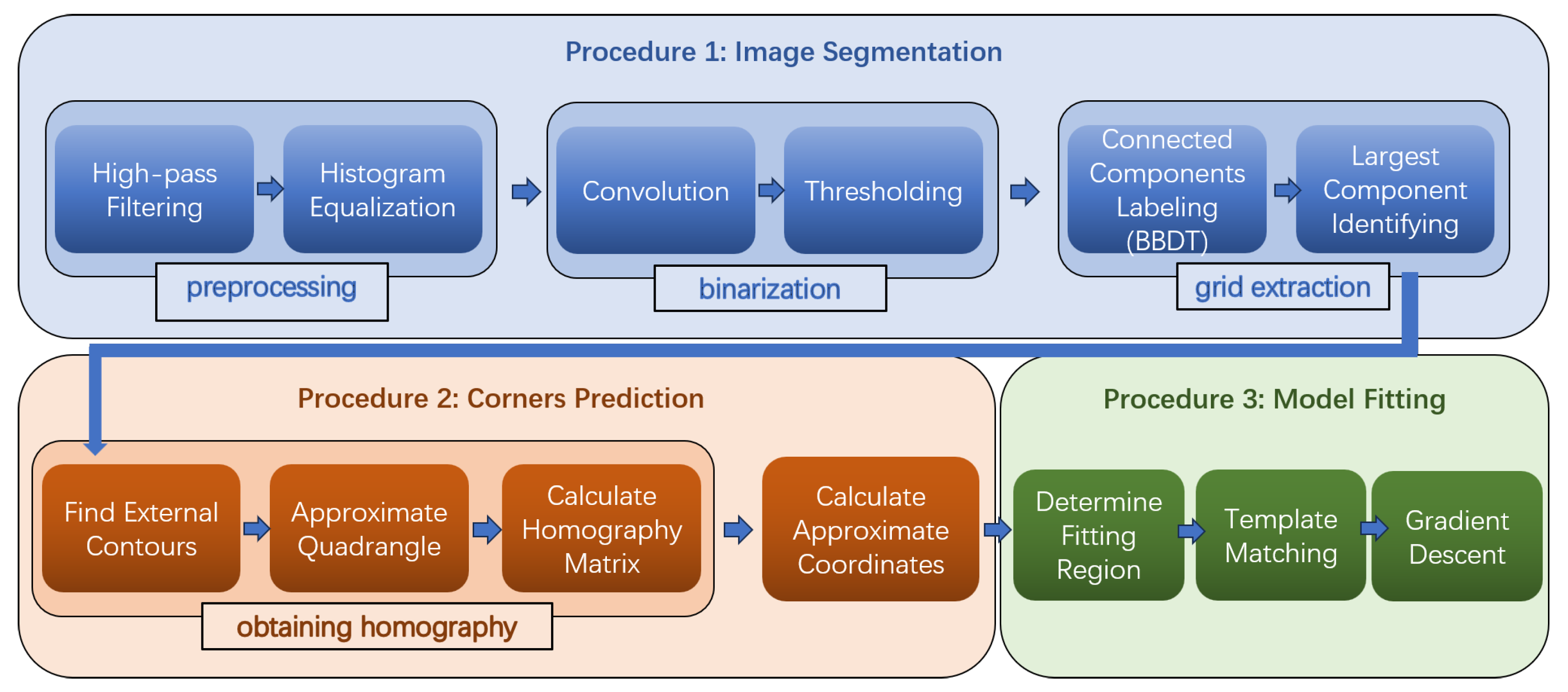
2. Methodology

Extensive studies have implemented corner detectors based on the intensity or the geometric information after image binarization. However, previous research may fail to detect corners due to the blurred edges caused by the shallow depth of field which is common in microscopic systems. As mentioned, the difference in the GESeF algorithm is the grid pattern and the segment-based strategy. It intends to handle the non-uniform illumination and blurring effect prior to corner detection. The characteristics of the grid pattern are utilized and a mathematical model describing the grid junction in binary images is established for precise corner detection.

The GESeF algorithm can be roughly divided into three procedures. Firstly, the grid pattern is extracted from the image. Secondly, a prediction procedure is performed to obtain approximate coordinates of grid junctions. Finally, the precise coordinates are obtained by performing model fitting on the segmentation result at each predicted coordinate. Figure 1 shows the procedures of the GESeF algorithm and the details of the algorithm will be discussed in subsequent content.

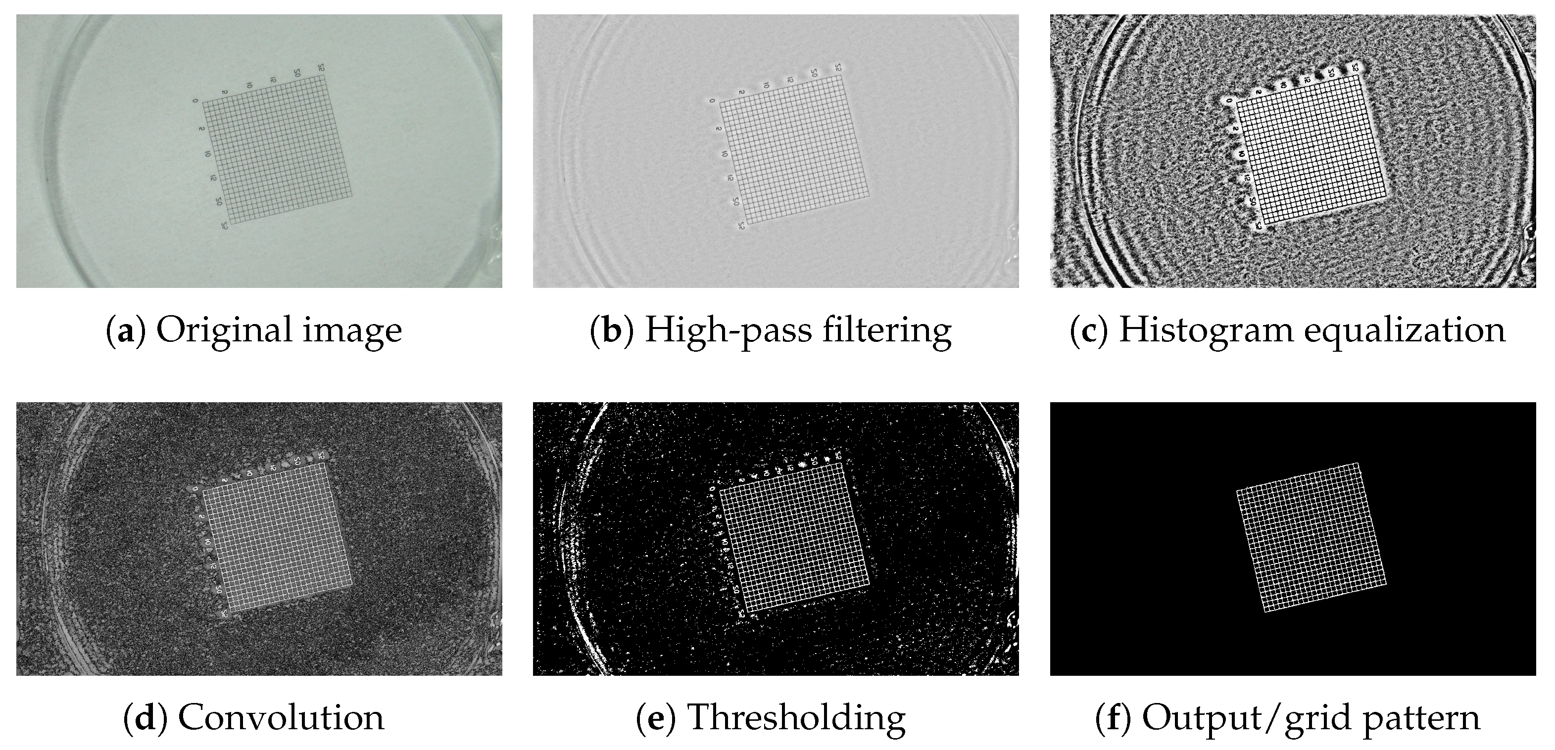
2.1. Segmentation Procedure

Image segmentation is one of the key issues of computer vision. A wide range of computer vision problems can take advantage of reliable and efficient image segmentation. Considering the high efficiency of obtaining a binary grid pattern through thresholding in uncluttered scenes, the thresholding-based segment method is used to extract the grid pattern in the captured images. Similarly to the image segmentation module in Figure 1, the segmentation method can be briefly divided into three steps: (1) image preprocessing, (2) thresholding, and (3) grid extraction.

In step 1, image preprocessing, the FFT (Fast Fourier Transform) is executed on the original image (Figure 2a) to obtain its spatial frequency. Subsequently, a circular high-pass filter was applied to this spatial frequency spectrum. After inverse Fourier transformation and histogram equalization, a high-contrast image that highlights the grid in the image is acquired, as shown in Figure 2c. The benefit of performing high-pass filtering and histogram equalization is that it reduces the influence of uneven illumination and improves the contrast of the grid pattern against the background.

In step 2, an image convolution was performed before thresholding. The absolute value of the difference between the intensity $I(x,y)$ of the pixel whose coordinate is $(x,y)$ and the average intensity $A(x,y)$ of a square region centered at pixel $(x,y)$ is calculated as the convolution result of pixel $(x,y)$; the response function $f(x,y)$ is shown in Equation (1),

$$f(x,y)=\left|I\right(x,y)-A(x,y\left)\right|$$

(1)

As shown in Figure 2d, the response function has a high intensity in the region that is significantly different from its surrounding pixels, i.e., those narrow and high-contrast regions. After convolution, thresholding is performed to extract those high-response regions, including the grid pattern and some redundant regions, as shown in Figure 2e.

In step 3, BBDT (Block-Based connected components labeling with Decision Tree) [20] is applied to label all the connected components in the binary image acquired by step 2. After labeling, the areas of all the connected components are acquired, and the largest connected component is identified as the segmentation result of the grid pattern, as shown in Figure 2f.

Figure 2 demonstrates that this segmentation method yields satisfactory results. During the image segmentation, the characteristics of the grid pattern are effectively utilized. Because of the narrowness of grid lines, convolution and thresholding processes can effectively segment the grid lines from the background. Furthermore, the grid pattern forms a single connected component, in contrast to the checkerboard pattern which consists of multiple independent squares. This property can be utilized to identify the grid in an uncluttered image. The subsequent procedures are all based on the segmentation result and the characteristics of the grid pattern will be further exploited.

2.2. Corner Prediction

To predict the coordinates of corners, the homography between the segmented grid and an assumed grid is utilized. The corner prediction procedure consists of two steps: (1) obtaining the homography matrix and (2) calculating the coordinates using the homography matrix. The corner prediction module in Figure 1 shows the workflow of the corner prediction procedure.

The homography matrix describes the correspondence of the coordinates between two planes in a perspective projection system. The homogeneous coordinate of a point $(x_2,y_2,1)$ on Plane-2 can be calculated from the homography matrix $\mathbf{H}$ and the homogeneous coordinate of the correspondence point $(x_1,y_1,1)$ on Plane-1 as Equation (2):

$$\lambda \left[\begin{array}{c}{x}_2\\ y_2\\ 1\end{array}\right]=\mathbf{H}\left[\begin{array}{c}{x}_1\\ y_1\\ 1\end{array}\right]=\left[\begin{array}{ccc}{h}_{11}& h_{12}& h_{13}\\ h_{21}& h_{22}& h_{23}\\ h_{31}& h_{32}& h_{33}\end{array}\right]\left[\begin{array}{c}{x}_1\\ y_1\\ 1\end{array}\right]$$

(2)

where $\mathbf{H}$ is a $3\times 3$ matrix and $\lambda$ is a scale factor produced by $\mathbf{H}$.

In order to obtain the homography matrix, at least four pairs of corresponding points in two planes are needed. Since the grid pattern has been obtained after segmentation, the four vertices of the grid can be utilized. Firstly, the external contour of the grid pattern is retrieved by the method proposed by Suzuki et al. [21]. Secondly, the Douglas–Peucker algorithm is applied to approximate a quadrangle representing the external contour of the grid pattern; Figure 3a shows the approximate quadrangle outlined by green lines. The four vertices of the approximated quadrangle are regarded as the four vertices of the grid pattern. After obtaining the coordinates of vertices, a set of initial coordinates assumptions, including vertex coordinates and corner coordinates, is generated based on the structure of the grid. The homography matrix is calculated according to the correspondence of initial vertex coordinates and the approximated vertex coordinates on the image. Finally, the predicted corner coordinates can be obtained by multiplying the homography matrix with the initial assumed corner coordinates. One of the predicted corners is shown in Figure 3b.

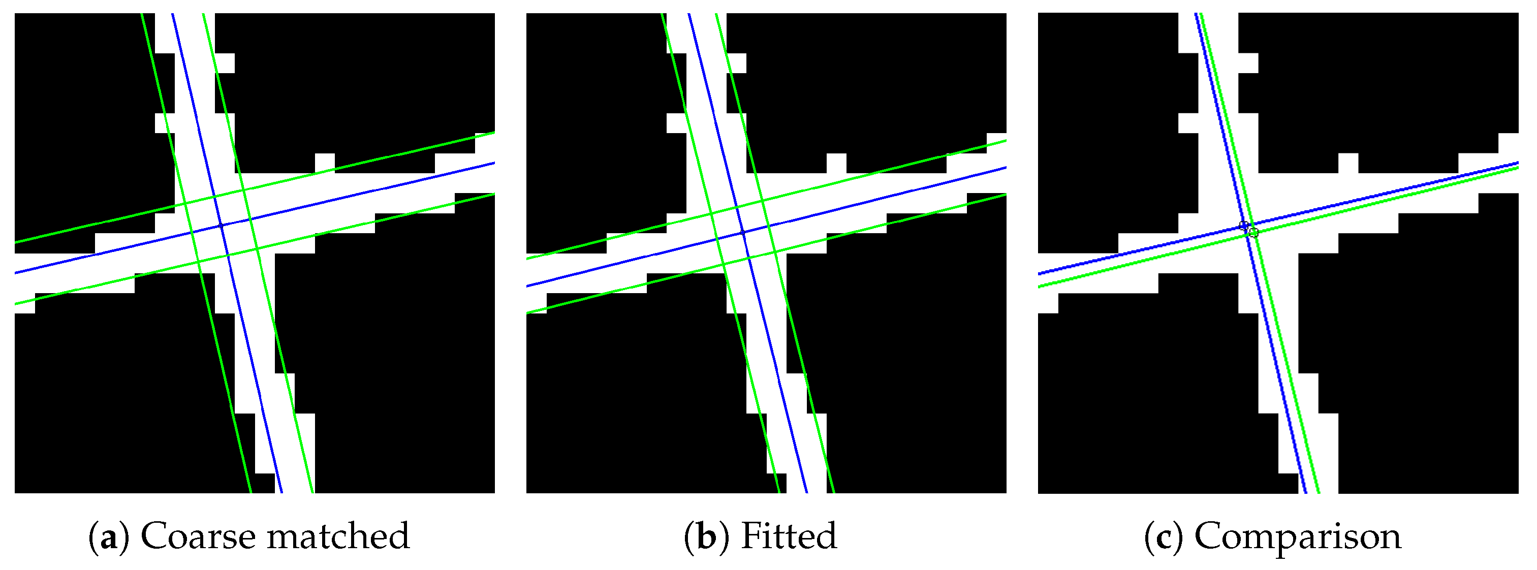
2.3. Model Fitting

The model fitting procedure adopts a coarse-to-fine strategy to locate the positions of corners. The model fitting module in Figure 1 depicts the schematic of the model fitting procedure. The whole model fitting procedure is applied in the vicinity of the predicted corner. Firstly, the fitting region is determined based on the predicted corner and the grid interval. A square region centered at the corner point, with a side length equal to the grid interval, is transformed together with the corner point (the green quadrangle in Figure 3b). The smallest rectangle region containing this transformed square is then selected as the fitting region. Secondly, a grid junction template is generated based on the predicted parameters and the established model, and then template matching is performed to obtain a coarse location of the corner in the matching region. Finally, gradient descent is applied to the cost function to obtain the optimal estimations of coordinates.

2.3.1. Mathematical Model of Grid Junction

The grid junction is the overlapping region where two lines intersect at a certain angle. In binary images, lines have a clear edge and a certain width. To describe these characteristics, the sigmoid function is utilized to establish the mathematical model. The sigmoid function is a logistic function that ranges from 0 to 1, making it suitable for describing the binary characteristic of a grid segment. The edges of lines can be approximated by the rising region of the sigmoid function, and the dramatic variation can be approximated by multiplying a scale factor on the independent variable of the sigmoid function. The width of lines can be constructed by multiplying the initial sigmoid function by its shifted symmetric function. Figure 4a shows the graph of the sigmoid function and the formula is given in Equation (3):

$$\sigma \left(x\right)={\displaystyle \frac{1}{1+e^{-x}}}$$

(3)

The two intersecting lines $L_1$ and $L_2$ can be represented as Equations (4) and (5), respectively:

$$L_1(x,y)=\sigma (s\times (l_1(x,y)+{\displaystyle \frac{b_1}{2}}))\times \sigma (-s\times (l_1(x,y)-{\displaystyle \frac{b_1}{2}}))$$

(4)

$$L_2(x,y)=\sigma (s\times (l_2(x,y)+{\displaystyle \frac{b_2}{2}}))\times \sigma (-s\times (l_2(x,y)-{\displaystyle \frac{b_2}{2}}))$$

(5)

where s is the scale factor, $b_1$ and $b_2$ are the widths of lines, and $l_1(x,y)$ and $l_2(x,y)$ are the functions of the distance to center line. In our implementation, the scale factor s is set to 10 to achieve a sharp rising edge that approximates the discontinuity of the line’s edge.

In this model, the angles between the center lines and the x-axis, denoted by ${\theta }_1$ and ${\theta }_2$ (with a range of $[0,\pi ]$), along with the coordinates of the junction $(c_x,c_y)$, are used to describe $l_1(x,y)$ and $l_2(x,y)$. Specifically, the equations for $l_1(x,y)$ and $l_2(x,y)$ are as follows:

$$l_1(x,y)=ycos{\theta }_1-xsin{\theta }_1-(c_{y}cos{\theta }_1-c_{x}sin{\theta }_1)$$

(6)

$$l_2(x,y)=ycos{\theta }_2-xsin{\theta }_2-(c_{y}cos{\theta }_2-c_{x}sin{\theta }_2)$$

(7)

Obviously, $l_1(x,y)=0$ and $l_2(x,y)=0$ are the formulas describing the center lines of two lines in the image. Unlike the general form of a line, which is represented by $Ax+By+C=0$, the two center lines can be described by four parameters $({\theta }_1,{\theta }_2,c_x,c_y)$ rather than six parameters $(A_1,B_1,C_1,A_2,B_2,C_2)$. This not only makes predicting initial values more intuitive but also reduces the computational complexity. Based on the established equations of the two lines, the mathematical model of the grid junction can be represented by Equation (8):

$$B(x,y)=1-(1-L_1(x,y))\times (1-L_2(x,y))$$

(8)

where $B(x,y)$ denotes the estimated intensity distribution at subpixel $(x,y)$. By reversing the distribution of 0 and 1 in Equations (4) and (5) and multiplying them, the structure of the two lines can be preserved as the 0-regions. Moreover, benefiting from the differentiability of the sigmoid function and the simple structure of $B(x,y)$, $B(x,y)$ becomes differentiable. This characteristic significantly aids in the subsequent fitting process. Figure 4b illustrates the function plot of $B(x,y)$, the green lines represent the two center lines $l_1(x,y)=0$ and $l_2(x,y)=0$, the red line is parallel to the x-axis, and the parameters are annotated in the plot.

2.3.2. Fitting Process

In the fitting process, a coarse-to-fine method is used to calculate the optimal estimates of the model. As $B(x,y)$ is determined by six parameters (${\theta }_1$, ${\theta }_2$, $c_x$, $c_y$, $b_1$, and $b_2$), we use a vector $\mathit{p}={({\widehat{\theta }}_1,{\widehat{\theta }}_2,{\widehat{c}}_x,{\widehat{c}}_y,{\widehat{b}}_1,{\widehat{b}}_2)}^T$ to denote the estimated parameters. For each corner point, the fitting region is unique and determined by the approach described earlier. After determining the fitting region (Figure 5a), the predicted $\mathit{p}$ is constructed based on the pose of the approximated quadrangle and the predicted coordinates.

For coarse fitting, a grid junction template image is generated by calculating the intensity distribution of $B(x,y)$ with the predicted $\mathit{p}$. The initial size of the template image is equal to the size of the fitting region. Considering the predicted coordinates probably deviate several pixels from the actual corner location, a template matching technique is applied to perform a coarse corner detection. For an $11\times 11$ pixel search scope, the outermost margin with a width of 5 pixels of the initial template is removed. Subsequently, the adjusted template is used for template matching within the fitting region. The displacement between the maximum pixeland the center pixel in the matching scores map (Figure 5c) represents the displacement of the coordinates between the coarse estimated coordinates and the predicted coordinates. After translating the predicted coordinates by this displacement, the coarse estimation of the corner is obtained. An instance is shown in Figure 5d, where the yellow lines denote the predicted two center lines, and the blue lines denote the two center lines after translation. It is obvious that the predicted coordinates deviate from the actual corner center, and the translated coordinates are closer to the actual corner center.

The more accurate fitting is performed by gradient decent. In the gradient descent process, a cost function denoted by the sum of squared residuals (SSR) is constructed as Equation (9):

$$SSR\left(\mathit{p}\right)=\sum {(b(x,y)-\widehat{B}(x,y;\mathit{p}))}^2$$

(9)

where the $b(x,y)$ denotes the intensity at the pixel $(x,y)$ in the fitting region. Since the cost function consists of several differentiable functions, the first-order partial derivatives with respect to each parameter can be easily calculated using the chain rule. In our implementation, the iterative method was applied and the $\mathit{p}$ at the k-th iteration is calculated as follows:

$${\mathit{p}}^{\left(k\right)}={\mathit{p}}^{(k-1)}-\gamma {\nabla }_{\mathit{p}}SSR\left({\mathit{p}}^{(k-1)}\right)$$

(10)

where the ${\mathit{p}}^{\left(k\right)}$ denotes the $\mathit{p}$ at the k-th iteration and $\gamma$ is the step size. After reaching the termination condition, the estimated parameters $({\widehat{c}}_x,{\widehat{c}}_y)$ represent the coordinates of the center point of the grid junction at a subpixel level. Figure 6 demonstrates the coarsely matched model and the fitted model. The green lines in Figure 6a,b represent the edges of the estimated model, and the blue lines represent the center lines of the estimated model. From Figure 6a we can see that the estimated center lines are close to the edges of the segmented lines, and the estimated edges also deviate from the edges of the segmented lines. After the gradient descent process, the estimated center lines and edges are more precise, as shown in Figure 6b. Figure 6c paints the matched center lines (blue lines) and fitted center lines (green lines) in the fitting region. From the comparison of the two estimated results, we can find that the gradient descent method significantly improves the precision of corner detection, which contributes to improving the precision of camera calibration.

3. Experimental Results

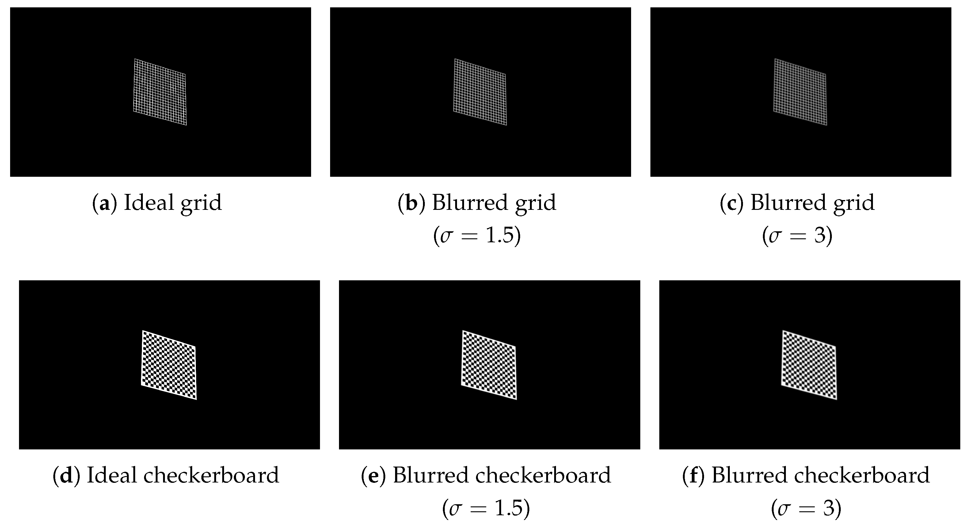
3.1. Detection Precision and Robustness

We used six sets of synthetic images to evaluate the accuracy of the proposed GESeF corner detector, as shown in Figure 7. Three sets are the grid pattern used for the proposed GESeF corner detector and others are the checkerboard pattern used for OpenCV’s corner detector. In the three grid pattern or checkerboard pattern sets, one set is ideal patterns with different orientations and others are the same images blurred by Gaussian kernel. The pattern has 19 × 19 = 361 corners and the resolution of each image is 1920 × 1080 pixels. The experiment was executed on the computer with an Intel Core i7-11370H CPU and 16 GB RAM.

Due to the simple composition of synthetic images, the image segmentation method in this experiment is thresholded with a threshold of 80. In the procedure of model fitting, the initial angle and corner center were calculated from the external contour of the segmented grid pattern, and the initial width of lines was set to 3 pixels. The search scope in the template matching process was 11 × 11 pixels. As for gradient descent, the iteration will end while the magnitude of the gradient of the cost function $\left|{\nabla }_{p}SSR\left(p^{(k-1)}\right)\right|<{10}^{-9}$ or the iterations exceed ${10}^4$.

In the experiment, each dataset has 75 images and the actual coordinates of corners are recorded while producing these images from a program. The blurred images were produced by applying Gaussian blurring on the ideal images, which has a kernel size of 9 × 9 with a standard deviation of 1.5 and 3. The results of the coordinate precision experiment are shown in

Table 1. Accuracy comparison.

Dataset	Standard Deviation	Method	Total Number of Corners	Average Error (Pixels)	Biggest Error (Pixels)
Ideal images	0	OpenCV	27,075	0.0802	0.2846
		Method in [22]	27,075	0.0621	0.4185
		GESeF	27,075	0.1193	0.4819
Blurred images	1.5	OpenCV	24,909	0.3595	4.5769
		Method in [22]	18,050	0.1688	1.0679
		GESeF	27,075	0.0930	0.4377
Blurred images	3	OpenCV	22,742	0.4978	2.9159
		Method in [22]	6859	0.2898	1.2968
		GESeF	27,075	0.1498	0.6747

Note: In blurred images, fewer corners are detected due to cases of detection failure.

.

The method in [22] is also a checkerboard corner detector proposed by Alexander Duda et al. and provided by OpenCV library. The absolute deviation in pixels between detected corners and actual corners was measured to evaluate the performance of different methods. The average error denotes the mean absolute deviation of all detected corners, and the biggest error denotes the maximum absolute deviation in all detected corners.

In Table 1, it can be found that the average error of our method is slightly higher than two checkerboard corner detectors in ideal images. However, for blurred images, the GESeF shows superior performance compared to the other two corner detectors. On one hand, the average error of the GESeF is much less than the other two methods. It is reasonable to deduce that the grid pattern is resistant to image blurring and leads to a lower average error, which is beneficial for camera calibration in microscopic scenes. On the other hand, the biggest error of the GESeF is less than the other two corner detectors in blurred images and even not exceeding 1 pixel, which means the GESeF has maintained the accuracy. Figure 8 shows one of the detected results in blurred images, the detected left-top corner severely deviates from the actual corner position in the checkerboard pattern, but the GESeF performs well on its counterpart. It is worth noting that the OpenCV’s corner detector and the method in [22] have detected fewer corners in blurred images due to several failed detections of checkerboard patterns, while our method has detected all the grid patterns and corners precisely. It means that the GESeF not only has high precision but is also more robust to image blurring.

3.2. Reprojection Error in Calibration and 3D Reconstruction

As a corner detector for the calibration pattern, it is necessary to evaluate the performance in the task of camera calibration. We performed camera calibration under the Mid SZ6100 stereo microscope (Midstereo, Guangzhou, China), and the magnification was 8×. Both the grid pattern and the checkerboard pattern were used for comparing calibration results. The resolution of images, which were captured by the built-in camera, is 1920 × 1080 pixels. Two kinds of patterns were used: one is the grid pattern with 24 × 24 corners and the interval is 0.20 mm, and the other is the checkerboard pattern with 19 × 15 corners and the interval is 0.25 mm, as shown in Figure 9. In the image segmentation procedure, the radius of the high-pass filter was 30 pixels, the window size of the convolution technique was set to 55 × 55 pixels, and the threshold T was 110.

To estimate the camera calibration accuracy, Zhang’s method [23] was applied to calculate camera parameters and the reprojection error. In this experiment, the OpenCV algorithm frequently fails to detect checkerboard corners, so we only compare the GESeF to the method described in [22]. The reprojection error of calibration against the two methods, the GESeF and the method in [22], are shown in

Table 2. Reprojection error.

Method	Pattern	Number of Images	Reprojection Error
Method in [22]	Checkerboard	40	0.332409
GESeF	Grid	40	0.172571

. The lower reprojection error means the corners detected by the GESeF have a better alignment to reprojected corners.

In order to validate the accuracy of the calibrated camera parameters, experiments of self-reconstruction and object-reconstruction were conducted. In the self-reconstruction experiment, the parameters of the dual camera system were calibrated using 40 pairs of checkerboard pattern images or 40 pairs of grid pattern images according to the used corner detector, method in [22] or the GESeF, respectively. After calibration, two calibration results were obtained and the images used for calibration were reloaded to perform 3D reconstruction of the pattern respectively. The corners were detected in the rectified image pair, and then the 3D structure of the corners was reconstructed based on triangulation. Finally, we compared the accuracy of two calibration results by measuring the intervals and diagonals of those reconstructed patterns. The MSE (mean squared error) of all fitted planes, which was estimated from reconstructed point clouds by the least squares method, was measured to evaluate the localization error of two corner detectors. The self-reconstruction result is shown in

Table 3. Self-reconstruction result.

Pattern	Actual Interval	Mean Interval	Error	Actual Diagonal	Mean Diagonal	Error	Plane MSE
Checkerboard	0.250000	0.250837	0.000837	5.700877	5.706677	0.005800	0.000123
Grid	0.200000	0.200275	0.000275	6.505382	6.509250	0.003868	0.000063

Unit: mm.

. The lower error of intervals and diagonals of the grid pattern means that the camera parameters obtained from the GESeF are more reliable. The MSE of the checkerboard pattern is even twice as large as the MSE of the grid pattern, which demonstrates that the GESeF has a smaller error range.

The object used in the object reconstruction experiment is a grid pattern with 9 × 9 corners, the interval is 0.50 mm, and the diagonal is 5.656854 mm. The corners were detected by the GESeF and reconstructed based on previously calibrated parameters. The mean interval and mean diagonal were measured to evaluate the accuracy of the calibrated parameters, and the results are shown in

Table 4. Grid reconstruction result.

Corner Detector Used in Calibration	Mean Interval	Error	Mean Diagonal	Error	Plane MSE
Method in [22]	0.501287	0.001287	5.670797	0.013943	0.000048
GESeF	0.500351	0.000351	5.659878	0.003024	0.000038

Unit: mm.

. The reconstructed point clouds, which used the GESeF as the corner detector in calibration, have lower errors. It demonstrates that the GESeF has higher precision and improves the calibration accuracy in the microscope. The MSE remains at a low level in both sets of point clouds demonstrating that the GESeF has a smaller error range once again.

3.3. Discussion

The GESeF performed well on both blurred images and captured photographs. As for the ideal images, the error is slightly higher than the other two algorithms because the clear edges benefit the corner detection of the checkerboard pattern. However, the difference between the three algorithms is not significant—the GESeF still maintains high accuracy on the ideal images. More importantly, blurring is inevitable in practical applications due to the point spread function of the optical system and the sampling of the sensor. In this regard, the GESeF is valuable for practical applications.

Despite its advantages, there are certain limitations to the GESeF. The corner prediction procedure is based on perspective transform, which does not account for distortion. For an image with severe distortion, the predictions may significantly deviate from the actual corners, leading to the selection of an incorrect fitting region. Additionally, the mathematical model describes straight lines, and curvature caused by distortion leads to deteriorated fitting results.

Although we only conduct the experiment with a microscope, it is also suitable for undistorted images of macro-scenes. Established mathematical models describe the general characteristics of two intersecting lines, indicating their potential for application in any scenario requiring the description of such patterns.

4. Conclusions

This paper developed a new method named GESeF for detecting grid junctions which can be utilized for calibrating stereo cameras in microscopes. The procedures and theory of this method have been demonstrated. The GESeF corner detector has combined the image segmentation with a model fitting process which directly utilizes the segmentation result to overcome the uneven illumination and shallow depth of view. Four experiments have been conducted. The average detecting error in synthetic images is less than 0.15 pixels, and the reconstruction error is less than 0.14% relative to the actual scale. A small location error for blurred images and a small reprojection error in camera calibration means that the GESeF is more robust. Experimental results show that the GESeF outperforms OpenCV’s checkerboard corner detector in blurred images and calibration accuracy. It indicates that our method has precise detection and is suitable for calibration in microscopic scenes due to its robustness against image blurring.

References

- Tserevelakis, G.J.; Tekonaki, E.; Kalogeridi, M.; Liaskas, I.; Pavlopoulos, A.; Zacharakis, G. Hybrid Fluorescence and Frequency-Domain Photoacoustic Microscopy for Imaging Development of Parhyale hawaiensis Embryos. Photonics 2023, 10, 264. [Google Scholar] [CrossRef]
- Wu, J.; Cai, X.; Wei, J.; Wang, C.; Zhou, Y.; Sun, K. A Measurement System with High Precision and Large Range for Structured Surface Metrology Based on Atomic Force Microscope. Photonics 2023, 10, 289. [Google Scholar] [CrossRef]
- Zhu, W.; Ma, C.; Xia, L.; Li, X. A Fast and Accurate Algorithm for Chessboard Corner Detection. In Proceedings of the 2009 2nd International Congress on Image and Signal Processing, Tianjin, China, 17–19 October 2009. [Google Scholar] [CrossRef]
- Juan, H.; Junying, X.; Xiaoquan, X.; Qi, Z. Automatic corner detection and localization for camera calibration. In Proceedings of the IEEE 2011 10th International Conference on Electronic Measurement & Instruments, Chengdu, China, 16–19 August 2011. [Google Scholar] [CrossRef]
- Guan, X.; Jian, S.; Hongda, P.; Zhiguo, Z.; Haibin, G. A Novel Corner Point Detector for Calibration Target Images Based on Grayscale Symmetry. In Proceedings of the 2009 Second International Symposium on Computational Intelligence and Design, Changsha, China, 12–14 December 2009. [Google Scholar] [CrossRef]
- Zhang, Y.; Li, G.; Xie, X.; Wang, Z. A new algorithm for accurate and automatic chessboard corner detection. In Proceedings of the 2017 IEEE International Symposium on Circuits and Systems (ISCAS), Baltimore, MD, USA, 28–31 May 2017. [Google Scholar] [CrossRef]
- Wang, Z.; Wang, Z.; Wu, Y. Recognition of corners of planar pattern image. In Proceedings of the 2010 8th World Congress on Intelligent Control and Automation, Jinan, China, 7–9 July 2010. [Google Scholar] [CrossRef]
- Shi, D.; Huang, F.; Yang, J.; Jia, L.; Niu, Y.; Liu, L. Improved Shi–Tomasi sub-pixel corner detection based on super-wide field of view infrared images. Appl. Opt. 2024, 63, 831–837. [Google Scholar] [CrossRef] [PubMed]
- Zhang, S.; Guo, C. A Novel Algorithm for Detecting both the Internal and External Corners of Checkerboard Image. In Proceedings of the 2009 First International Workshop on Education Technology and Computer Science, Wuhan, China, 7–8 March 2009. [Google Scholar] [CrossRef]
- Bennett, S.; Lasenby, J. ChESS—Quick and Robust Detection of Chess-board Features. Comput. Vis. Image Underst. 2014, 118, 197–210. [Google Scholar] [CrossRef]
- Huang, L.; He, L.; Li, J.; Yu, L. A Checkerboard Corner Detection Method Using Circular Samplers. In Proceedings of the 2018 IEEE 4th International Conference on Computer and Communications (ICCC), Chengdu, China, 7–10 December 2018. [Google Scholar] [CrossRef]
- Sang, Q.; Huang, T.; Wang, H. An improved checkerboard detection algorithm based on adaptive filters. Pattern Recognit. Lett. 2023, 172, 22–28. [Google Scholar] [CrossRef]
- Yimin, L.; Naiguang, L.; Xiaoping, L.; Peng, S. A novel approach to sub-pixel corner detection of the grid in camera calibration. In Proceedings of the 2010 International Conference on Computer Application and System Modeling (ICCASM 2010), Taiyuan, China, 22–24 October 2010. [Google Scholar] [CrossRef]
- Placht, S.; Fürsattel, P.; Mengue, E.A.; Hofmann, H.; Schaller, C.; Balda, M.; Angelopoulou, E. ROCHADE: Robust Checkerboard Advanced Detection for Camera Calibration. In Proceedings of the Computer Vision—ECCV 2014, Zurich, Switzerland, 6–12 September 2014; Fleet, D., Pajdla, T., Schiele, B., Tuytelaars, T., Eds.; Springer: Cham, Switzerland, 2014; pp. 766–779. [Google Scholar]
- Feng, W.; Wang, H.; Fan, J.; Xie, B.; Wang, X. Geometric Parameters Calibration of Focused Light Field Camera Based on Edge Spread Information Fitting. Photonics 2023, 10, 187. [Google Scholar] [CrossRef]
- Du, X.; Jiang, B.; Wu, L.; Xiao, M. Checkerboard corner detection method based on neighborhood linear fitting. Appl. Opt. 2023, 62, 7736–7743. [Google Scholar] [CrossRef] [PubMed]
- Donné, S.; De Vylder, J.; Goossens, B.; Philips, W. MATE: Machine Learning for Adaptive Calibration Template Detection. Sensors 2016, 16, 1858. [Google Scholar] [CrossRef] [PubMed]
- Wu, H.; Wan, Y. A highly accurate and robust deep checkerboard corner detector. Electron. Lett. 2021, 57, 317–320. [Google Scholar] [CrossRef]
- Zhu, H.; Zhou, Z.; Liang, B.; Han, X.; Tao, Y. Sub-Pixel Checkerboard Corner Localization for Robust Vision Measurement. IEEE Signal Process. Lett. 2024, 31, 21–25. [Google Scholar] [CrossRef]
- Grana, C.; Borghesani, D.; Cucchiara, R. Optimized Block-Based Connected Components Labeling With Decision Trees. IEEE Trans. Image Process. 2010, 19, 1596–1609. [Google Scholar] [CrossRef] [PubMed]
- Suzuki, S. Topological structural analysis of digitized binary images by border following. Comput. Vision Graph. Image Process. 1985, 30, 32–46. [Google Scholar] [CrossRef]
- Duda, A.; Frese, U. Accurate Detection and Localization of Checkerboard Corners for Calibration. In Proceedings of the British Machine Vision Conference, Newcastle, UK, 3–6 September 2018. [Google Scholar]
- Zhang, Z. A flexible new technique for camera calibration. IEEE Trans. Pattern Anal. Mach. Intell. 2000, 22, 1330–1334. [Google Scholar] [CrossRef]