Microscopic Temperature Sensor Based on End-Face Fiber-Optic Fabry–Perot Interferometer

Abstract

This work proposes a simple and affordable technology for the manufacturing of a miniature end-face fiber-optic temperature sensor based on a Fabry–Perot interferometer formed from a transparent UV-curable resin. For the manufactured working prototype of the sensor, the sensitivity and operating temperature range were determined, and the methods for their enhancement were proposed. Due to its small size, the proposed type of sensor can be used in high-precision and minimally invasive temperature measurements, in biology for microscale sample monitoring, and in medicine during operations using high-power lasers. A microwave photonic method is proposed that enables the interrogation of the sensor without using an optical spectrum analyzer.

1. Introduction

The creation of simple and affordable fiber-optic temperature sensors, both in design and in the interrogation method, is undoubtedly a very relevant direction in fiber-optic sensor development. The main advantages of such sensors are their resistance to electromagnetic interference, low weight and size, multiplexing capability, and high sensitivity [1]. The industry has proposed many variations of the sensitive part of a fiber-optic temperature sensor based on a fiber Bragg grating [2,3,4,5,6] and various types of interferometers [7,8,9,10,11,12]. Of all the interferometers, the fiber-optic Fabry–Perot interferometer (FPI) is of particular interest, since it features a simple design, compactness, high sensitivity, and good performance at high temperatures [13,14,15], and it enables high interrogation speed coupled with low inertia. The main methods for the formation of sensors based on a Fabry–Perot interferometer are the combination of several structures of photonic crystal fibers [16] or hollow core fibers [17,18]; however, these components are very specific and have a high price, which increases the cost of the final product. It is also noteworthy that due to the relatively small values of the thermo-optic coefficient and the coefficient of thermal expansion of quartz glass, the sensors solely formed from such material have a limited sensitivity, not exceeding ~14 pm/°C [14].

To increase the sensitivity, various technical solutions have been proposed that utilize materials with higher thermo-optic and/or thermal expansion coefficients. Thus, in [19], a Fabry–Perot interferometer composed of a silicon cylinder was presented, which was manufactured using deep reactive ion plasma etching and demonstrated a sensitivity of ~85 pm/°C. In [20], an FPI was formed by filling a section of a hollow fiber with polydimethylsiloxane (PDMS), which, in combination with the Vernier effect, increased the sensitivity up to 650 pm/°C. An even higher sensitivity of ~2.87 nm/°C was reported in [21], where a similar cascaded polymer-filled (NOA65) FPI was developed, also employing the Vernier effect. Another approach involving a sealed cavity filled with ethanol inside an optical fiber [22] demonstrated a temperature sensitivity of ~430 pm/°C at the cost of a more complicated manufacturing process. A comparison between some of the existing sensors and the proposed one is presented in

Table 1. A comparison between some of the existing temperature sensors and the proposed sensor.

Sensor	Length, μm	Lateral Dimension, μm	Sensitivity, pm/°C	Reference
Fiber Bragg grating	~1 × 103–1 × 104	125	~10	[23,24]
Microfiber tip FPI	~60–360	~30	~14	[14]
Silicon pillar FPI	~200	~80	~85	[19]
FPI based on hollow fiber with PDMS	~34 + 138	~130	~650 *	[20]
Cascaded FPI with NOA65	~78 + 84	~150	~2.87 × 103 *	[21]
Ethanol-filled FPI	~24–45 + 150	~125	~430	[22]
Proposed sensor	~40–90	~20–50	~44	–

* Increased with the Vernier effect.

.

In this work, we propose to form a Fabry–Perot interferometer at the end of an optical fiber from an affordable and widespread photopolymer material using a simple manufacturing method. The proposed sensor features significantly higher sensitivity in comparison with fiber Bragg gratings and quartz glass-based FPIs, as well as a smaller size and simpler manufacturing process compared to Bragg gratings, silicon pillar, and hollow fiber-based FPIs, which can be beneficial in areas where the usage of minimally invasive sensors is necessary, such as medical and biological applications.

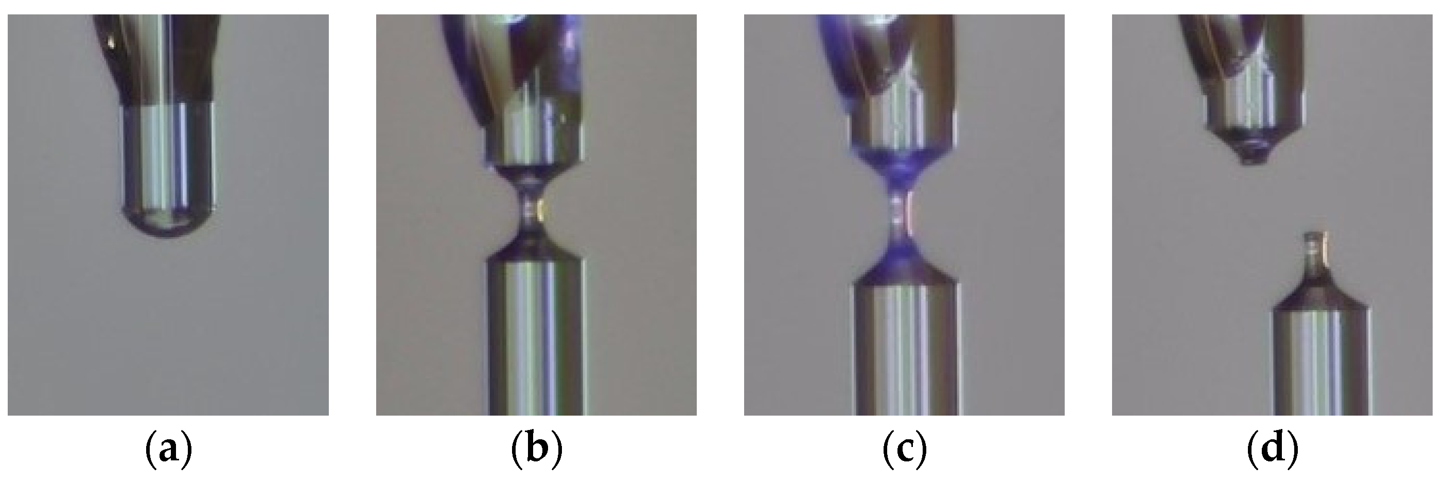
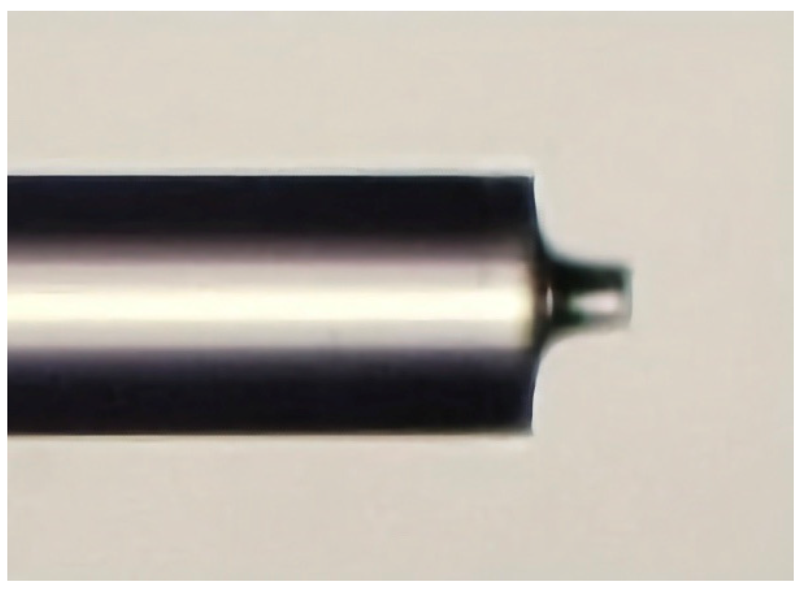
2. The Formation of the Sensitive Element

As a material for the sensitive part of the temperature sensor, it was proposed to use a photosensitive polymer that is transparent to visible light and the near-IR range and cured under the influence of ultraviolet (UV) radiation. The process of forming the sensor is based on the technique of forming a polymer “bridge” [25] between the end faces of two optical fibers. Firstly, the ends of two single-mode fiber-optic pigtails are stripped of the protective and strengthening coating, the remaining acrylate coating is removed from the fibers, and the ends of the fibers are cleaved at right angles. The prepared fibers are placed in holders mounted on micropositioners opposite each other. A radiation source (1550 nm) is connected to one of the pigtails, and an optical power meter is connected to the other pigtail (Figure 1). Under a microscope and using an optical power meter, the optical fibers are precisely adjusted to position them coaxially and opposite each other.

After alignment, the optical fibers are spaced a certain distance (~3 mm) apart, and a drop of photopolymer material is applied to the end of one of the pigtails using the LongerPump TS-2A liquid dosing system (Figure 2a).

When the opposite optical fiber is approached, due to the wettability of the fiber and surface tension forces, the polymer is stretched between the ends of the optical fibers, and as a result, a “bridge” of polymer material is formed between the end faces of the fibers. The polymerization process occurs through step-by-step alternate irradiation with an ultraviolet source FUWO (FUV-6L) and the separation of optical fibers (Figure 2b,c). Controlling the speed and distance of separation and duration and power of radiation at each stage allows us to manage the length, thickness, and shape of the resulting structure. Cleaving the resulting polymer bridge close to one of the ends (Figure 2d) ensures the formation of a “column” with a perpendicular end face. Thus, two interfaces—optical fiber/polymer and polymer/air—together form a Fabry–Perot interferometer at the end of the fiber (Figure 3).

The reflection spectrum of the sensitive element was investigated using a setup consisting of a superluminescent fiber source—1, a circulator—2, and an optical spectrum analyzer EXFO OSA20—3, Figure 4a. The emission spectrum of a superluminescent fiber source (1510–1580 nm with an output power of up to 4 mW) is shown in Figure 4b, and the reflection spectrum of the sensitive element depicted in Figure 3 is presented in Figure 4c.

To assess the possibility of using the proposed sensitive element as a temperature sensor, measurements of the spectrum were carried out when the temperature in the climate chamber changed, as discussed in Section 4.

3. The Mathematical Modeling of the Sensing Element

3.1. Method for Sensing Element Modeling

In order to estimate the spectral response of the proposed sensing element and evaluate its sensitivity, a mathematical model of the Fabry–Perot interferometer is utilized, which is based on the apparatus of scattering and transmission matrices [26,27]. The sensing element is represented as a sequential combination of three uniform media: the optical fiber, polymer “column”, and ambient air. The reflection spectrum of the interferometer is modeled by the multiplication of three transfer matrices: (1) a stepwise change in the propagation medium parameters (transition from the optical fiber core to the polymer); (2) a uniform medium of the polymer “column” (inner cavity of the interferometer); and (3) another stepwise change in the propagation medium parameters (transition from the polymer cavity to the ambient air). The scattering matrix of a uniform continuous medium is formulated as a function of the permittivity, permeability, and length of the medium and the wavelength of propagating radiation [26,27]:

$$S_{\mathrm{M}}=\left[\begin{array}{cc}0& e^{-j\cdot H\cdot \gamma }\\ e^{-j\cdot H\cdot \gamma }& 0\end{array}\right],$$

(1)

where

$$\gamma ={\displaystyle \frac{\pi }{\lambda }}\sqrt{2\mathrm{Re}\epsilon \cdot \mathrm{Re}\mu }\left(\sqrt{\sqrt{1-{\left({\displaystyle \frac{\mathrm{Im}\epsilon }{\mathrm{Re}\epsilon }}\right)}^2}+1}-j\sqrt{\sqrt{1-{\left({\displaystyle \frac{\mathrm{Im}\epsilon }{\mathrm{Re}\epsilon }}\right)}^2}-1}\right).$$

(2)

In (2), ε and μ are the permittivity and permeability of the uniform medium, H is the length of the medium, and λ is the wavelength of propagating radiation.

The scattering matrices of the stepwise change in the medium parameters at the interfaces of different media are formulated using the permittivities and permeabilities of the media:

$$S_{\mathrm{J}}^{12}=\left[\begin{array}{cc}{\displaystyle \frac{\sqrt{{\epsilon }_1{\mu }_2}-\sqrt{{\mu }_1{\epsilon }_2}}{\sqrt{{\mu }_1{\epsilon }_2}+\sqrt{{\epsilon }_1{\mu }_2}}}& {\displaystyle \frac{2\cdot \sqrt[4]{{\epsilon }_1{\mu }_1{\epsilon }_2{\mu }_2}}{\sqrt{{\mu }_1{\epsilon }_2}+\sqrt{{\epsilon }_1{\mu }_2}}}\\ {\displaystyle \frac{2\cdot \sqrt[4]{{\epsilon }_1{\mu }_1{\epsilon }_2{\mu }_2}}{\sqrt{{\mu }_1{\epsilon }_2}+\sqrt{{\epsilon }_1{\mu }_2}}}& {\displaystyle \frac{\sqrt{{\epsilon }_1{\mu }_2}-\sqrt{{\mu }_1{\epsilon }_2}}{\sqrt{{\mu }_1{\epsilon }_2}+\sqrt{{\epsilon }_1{\mu }_2}}}\end{array}\right], S_{\mathrm{J}}^{23}=\left[\begin{array}{cc}{\displaystyle \frac{\sqrt{{\epsilon }_2{\mu }_3}-\sqrt{{\mu }_2{\epsilon }_3}}{\sqrt{{\mu }_2{\epsilon }_3}+\sqrt{{\epsilon }_2{\mu }_3}}}& {\displaystyle \frac{2\cdot \sqrt[4]{{\epsilon }_2{\mu }_2{\epsilon }_3{\mu }_3}}{\sqrt{{\mu }_2{\epsilon }_3}+\sqrt{{\epsilon }_2{\mu }_3}}}\\ {\displaystyle \frac{2\cdot \sqrt[4]{{\epsilon }_2{\mu }_2{\epsilon }_3{\mu }_3}}{\sqrt{{\mu }_2{\epsilon }_3}+\sqrt{{\epsilon }_2{\mu }_3}}}& {\displaystyle \frac{\sqrt{{\epsilon }_2{\mu }_3}-\sqrt{{\mu }_2{\epsilon }_3}}{\sqrt{{\mu }_2{\epsilon }_3}+\sqrt{{\epsilon }_2{\mu }_3}}}\end{array}\right],$$

(3)

where ε₁ and μ₁ are the permittivity and permeability of the optical fiber, ε₂ and μ₂ are the same parameters of the interferometer cavity (polymer “column”), and ε₃ and μ₃ are the same parameters of the ambient medium (air).

The transfer matrix T can be calculated from the scattering matrix S and vice versa using the following operators [26]:

$$\overleftrightarrow{\mathbf{T}}\left(S\right)={\displaystyle \frac{1}{S_{2,1}}}\left(\begin{array}{cc}{S}_{2,1}{S}_{1,2}-S_{1,1}{S}_{2,2}& S_{1,1}\\ -S_{2,2}& 1\end{array}\right),\overleftrightarrow{\mathbf{S}}\left(T\right)={\displaystyle \frac{1}{T_{2,2}}}\left(\begin{array}{cc}{T}_{1,2}& T_{1,1}{T}_{2,2}-T_{1,2}{T}_{2,1}\\ 1& T_{2,1}\end{array}\right).$$

(4)

The resulting transfer matrix of the whole sensitive element is derived by the sequential multiplication of the transfer matrices of the cavity interfaces and the polymer cavity medium of the interferometer and is formulated as a function of the propagating radiation wavelength, permittivities and permeabilities of the media, and cavity length [26]:

$$T^{\mathrm{FP}}=T_{\mathrm{J}}^{12}\times T_{\mathrm{M}}^2\times T_{\mathrm{J}}^{23}.$$

(5)

In (5), the lower index denotes the transfer matrix (“J” is a stepwise change in parameters, “M” is uniform medium), the upper index of the matrices denotes the ordinal number of layers, and in the matrices “J”, it indicates the direction of radiation transition from the i-th layer to the (i + 1)-th layer.

The scattering matrix of the Fabry–Perot interferometer S^FP is derived from the transfer matrix T^FP using the operator (4):

$$S^{\mathrm{FP}}={\displaystyle \frac{1}{{\left(T^{\mathrm{FP}}\right)}_{2,2}}}\left(\begin{array}{cc}{\left(T^{\mathrm{FP}}\right)}_{1,2}& ‖T^{\mathrm{FP}}‖\\ 1& {\left(T^{\mathrm{FP}}\right)}_{2,1}\end{array}\right).$$

(6)

Each of the elements of the scattering matrix S^FP defines the reflection or transmittance coefficients of the interferometer for the light propagating in different directions. The element (S^FP)_1,1 of the resulting scattering matrix defines the reflection coefficient for radiation directed into the interferometer from the optical fiber side (“forward” direction); (S^FP)_2,2 is the reflection coefficient in the opposite (“reverse”) direction; (S^FP)_1,2 is the transmittance coefficient in the “forward” direction; and (S^FP)_2,1 is the transmittance coefficient for radiation in the “reverse” direction. In general, all reflection and transmission coefficients are functions of the wavelength, permittivities and permeabilities of all media, and the length of the interferometer cavity.

The variation in ambient temperature causes changes in all seven parameters of the interferometer: the permittivities (ε) and permeabilities (μ) of the three media (which alter the refractive index n of the media as $n=\sqrt{\epsilon \mu }$) as well as the length of the interferometer inner cavity. Since the first medium is quartz glass (optical fiber), the second one is a polymer (dielectric), and the external medium is air, then the temperature variation only changes the dielectric permittivity and the length of the interferometer cavity [28].

To model the effect of temperature variation on the parameters of the sensor, the linear dependence of the media refractive index and the interferometer length on the temperature change is used:

$$n_i\left(T\right)=n_i\left(1+(d{n}_i/dT)\cdot \Delta T\right),i=1,2,H\left(T\right)=H_0\left(1+\alpha \cdot \Delta T\right),$$

(7)

where dn_i/dT is the temperature-caused refractive index variation (thermo-optic coefficient) in the i-th medium, α is the coefficient of thermal expansion of the polymer “column”, n_i is the refractive index of the i-th medium, and H₀ is the length of the interferometer inner cavity (polymer “column”) at the reference temperature.

3.2. Modeling Results

The parameters of the media used during the modeling are listed in

Table 2. The modeling parameters of the sensing element.

Parameter	Value
Refractive index of the optical fiber (n1), RIU	1.4587
Refractive index of the interferometer cavity (n2), RIU	1.59
Length of the interferometer cavity (H0), m	51.22 × 10−6
Thermo-optic coefficient of the optical fiber (dn1/dT), °C−1	8.6 × 10−6
Thermo-optic coefficient of the interferometer cavity (dn2/dT), °C−1	−1.87 × 10−4
Thermal expansion coefficient of the interferometer cavity (α), °C−1	1.6 × 10−4

.

Figure 5 presents the modeled reflection spectrum of the sensitive element with the temperature varied in the range of 25 °C.

As can be seen from Figure 5, the spectral response of the modeled sensor shifts towards a shorter wavelength, and its maximum reflectance value slightly decreases. The shift in the spectral peak near 1530 nm with the increase in temperature is illustrated in Figure 6, where linear data approximation is also shown (blue dashed line). The resulting sensitivity of the spectrum shift is estimated to be ~0.0446 nm/°C.

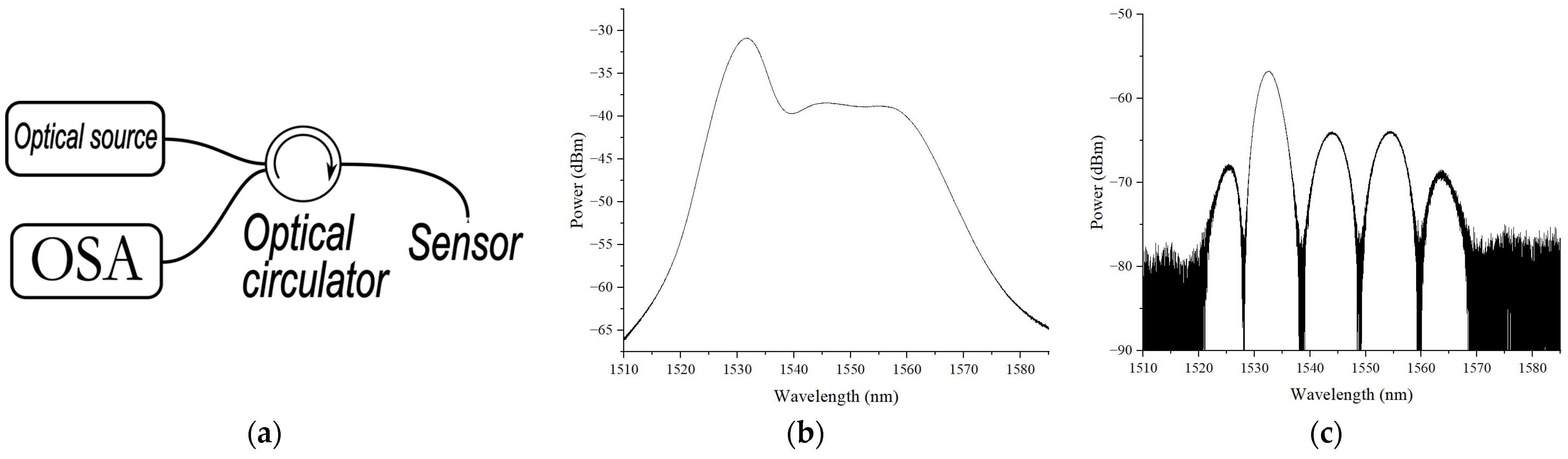
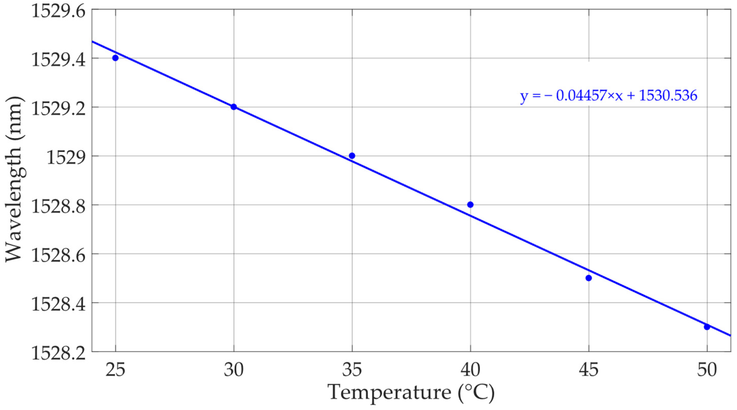
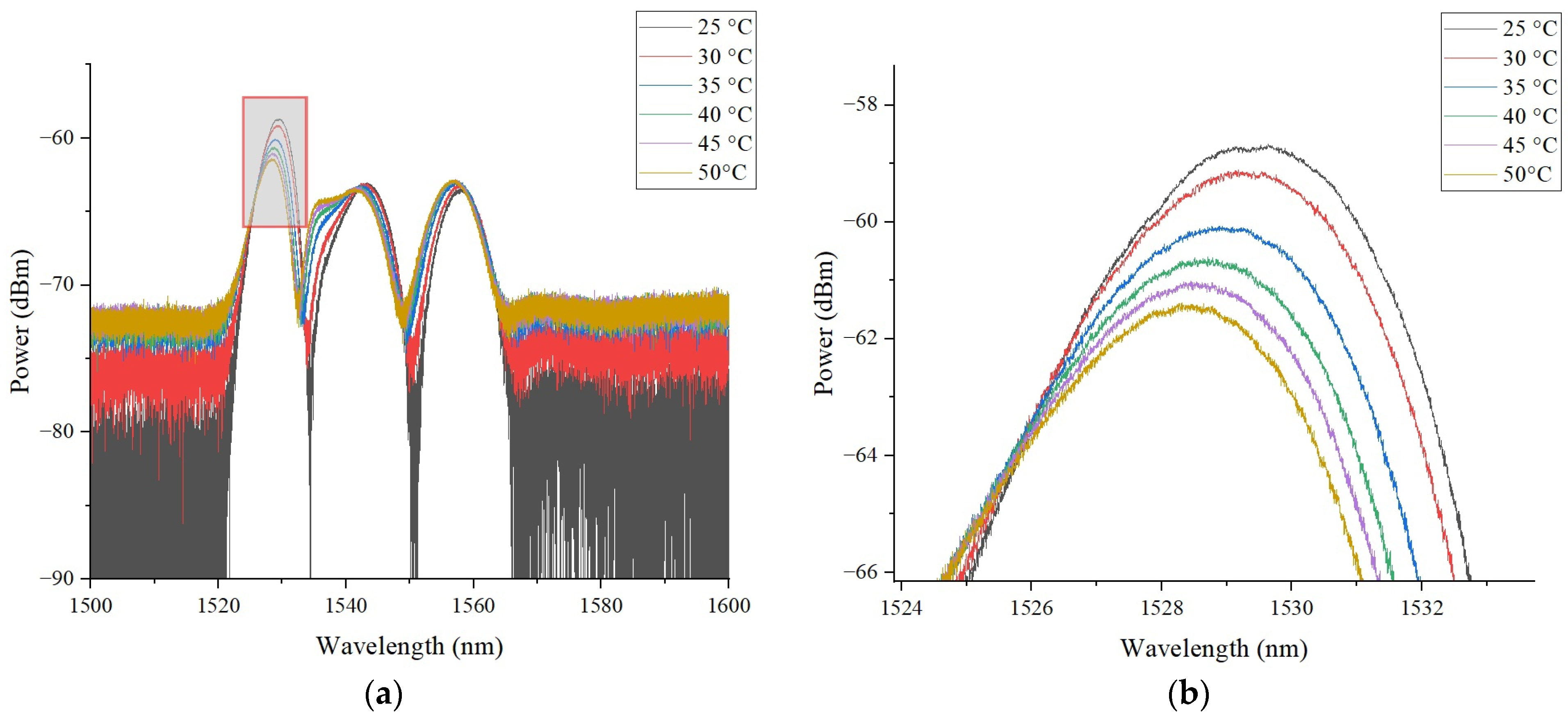
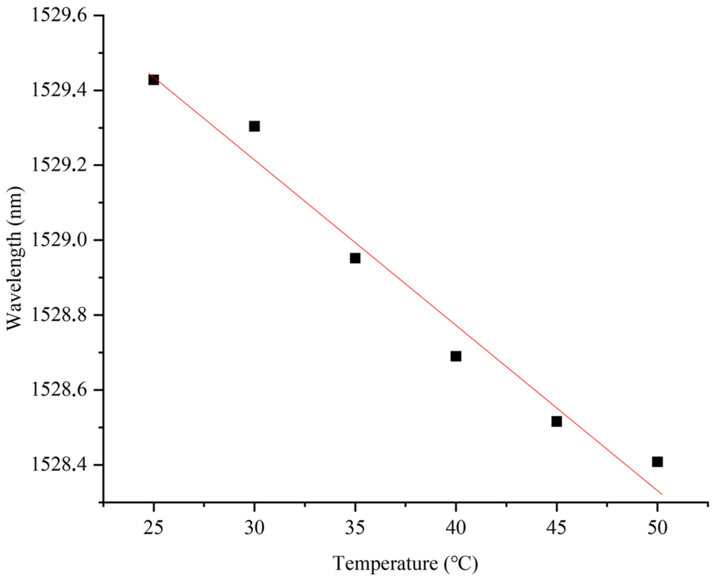
4. Temperature Tests

The subject of the temperature tests was a sensitive element in the form of the polymer “column” manufactured from UV-curable epoxy AC545, as described in Section 2, and having the following dimensions: a diameter of 32 μm and length of 51.2 μm (Figure 7).

The sensor was placed inside a climatic chamber 60/150-80 KTX; the temperature inside the climatic chamber varied linearly from 30 to 50 °C in steps of 5 °C with a heating rate of 4 °C/min and holding time of 5 min at each step. The reflection spectra of the sensor at different temperatures are presented in Figure 8.

As predicted by the theory of fiber-optic Fabry–Perot interferometers [28], when the temperature changes, the shape of the reflection spectrum is maintained, but the spectrum itself shifts along the wavelength. The experimental data obtained make it possible to determine the shift in the reflection spectrum with high accuracy and, consequently, the temperature acting on the sensitive element, as demonstrated in Figure 8.

The monotonic shift in the spectrum when the external temperature changes (Figure 9) allows the proposed sensing element to be used as a precision temperature sensor, the sensitivity of which is ~44.1 pm/°C, exceeding the sensitivity of classical fiber-optic sensors (~11 pm/°C), the sensitive element of which is based on quartz glass.

The performed experiments confirm a linear shift in the reflection spectrum with an increase in temperature acting on the sensitive element, which is in good agreement with the previous results attained by the authors and the data of other researchers [28,29]. The obtained dependence confirms the possibility of using the developed sensitive element in the specified temperature range.

5. Ensuring High Interrogation Speed at Low Cost of Sensor System

The interrogation of the proposed sensor can be carried out using a microwave photonic method that includes the generation of an optical frequency comb, which in general consists of two or more ultra-narrowband spectral components separated by a frequency of the order of several GHz and is used to probe the spectrum of a Fabry–Perot interferometer (Figure 10). An optical frequency comb can be formed by modulating laser radiation with a radio frequency signal or by passing broadband optical radiation through a specially structured fiber Bragg grating [30].

At the photodetector, cross-beats of all components of the optical frequency comb radiation occur. The shift in the FPI spectrum caused by temperature variation entails a change in the amplitudes of the reflected spectral components of the optical frequency comb, the spectral position of which is assumed to be stabilized in the middle of the linear section of the interferometer spectrum. This, in turn, leads to a change in the amplitudes of the beating signal at the output of the photodetector. The values of amplitudes can be analyzed using the apparatus of artificial neural networks (ANNs) to define the shift in the FPI spectrum. In this case, the sampling frequency of the FPI is only limited by the performance of the analog-to-digital converter and the processor that calculates the position of the FPI spectrum, and it can reach tens or hundreds of kHz.

In the current work, the microwave photonic interrogation of the proposed FPI was modeled similarly to [30]. The probing radiation was modeled as the five-component optical frequency comb spectrum, each component of which was described by a normal distribution function, with a common envelope also described by a normal distribution function. The resulting electrical signal of the photodetector was modeled according to [30] and was used to create a sample for artificial neural network training aimed at temperature detection. To train the artificial neural network, microwave photonic processing data were generated for temperature values varying in the range from 23 to 52 °C with a discrete step ΔT = 0.001 °C and with added noise of 1/f type not exceeding 0.1% of the signal amplitude. As a result, a marked-up set of 29,100 data points was obtained, which were normalized into the dimensionless interval [0; 1] to form a normalized set of input and output data for training.

Several configurations of a fully connected ANN were tested, in all of which the input layer consisted of four neurons, while the output layer consisted of one neuron. The logistic activation function was used for training. The accuracy of the model was assessed using two parameters, the mean absolute error (MAE) and the mean relative error (MRPE), calculated as follows:

$$MAE={\displaystyle \frac{1}{M}}{\displaystyle \sum _{i=1}^M\left|y_i-p_i\right|}, MRPE={\displaystyle \frac{1}{M}}{\displaystyle \sum _{i=1}^M\frac{\left|y_i-p_i\right|}{y_i}\cdot 100\%},$$

(8)

where M is the number of data in the data set, y_i is the actual value, and p_i is the predicted value for the i-th data set. Several of the tested configurations are listed in

Table 3. Error values for various configurations of ANN. The utilized configuration is highlighted in bold.

No. of ANN	No. of Hidden Layers	No. of Neurons in Each Hidden Layer	MAE, °C
(1)	1	50	5
(2)	1	200	4
(3)	2	50/20	3.5
(4)	2	100/50	3
(5)	3	50/20/20	2
(6)	3	150/100/50	1.5
(7)	4	300/200/150/100	0.3
(8)	5	800/500/400/300/150	0.008
(9)	5	1500/1200/1000/500/400	0.002

, where the corresponding MAE values were obtained in the temperature range from 23 to 52 °C.

In this study, configuration No. 8 from Table 3 was used, which is a fully connected ANN corresponding to sensing with an optical frequency comb containing five frequency components, the input layer of which consisted of 4 neurons, followed sequentially by hidden layers containing 800, 500, 400, 300, and 150 neurons, respectively. The output layer consisted of one neuron. In this case, a linear activation function was used for the first three layers, and Relu, linear, and Relu were used for layers 4, 5, and the output layer, respectively. The ANN was implemented using Python 3.11 with the TensorFlow library.

As required by the learning algorithms, the labeled data set was divided into a training data set (90%) and a control data set (10%). The training data set was used directly to adjust the weights, while the control data set was used to determine the accuracy of the model between training iterations. The model was trained in two stages. The first stage included 400 iterations of training using the Adam optimization algorithm with a reduction in the learning rate to 0.001. As a result, the value of the loss function did not exceed 0.05. The second stage included additional training of the model for 400 iterations with a gradual decrease in the learning rate to 1 × 10⁻⁶. As a result, the maximum value of the loss function on the training set did not exceed 2 × 10⁻⁴.

The values of absolute and relative errors in temperature determination are given in

Table 4. Error values for temperature determination in various ranges using the developed ANN.

Range, °C	MAE, °C	MRPE, %
from 23 to 52	0.03214	0.06459
from 24 to 51	0.01542	0.02172
from 25 to 50	0.008358	0.018271
from 26 to 49	0.00378	0.00912
from 27 to 48	0.002372	0.00662

below.

The obtained data show that the trained ANN model demonstrated the maximum error at the largest verifiable range, and as the range decreased, the error value decreased significantly to 0.002 °C. In the considered temperature range from 25 to 50 °C, the absolute error was ~0.008 °C, which can be assessed as high accuracy.

6. Discussion and Conclusions

As a result of this research, theoretical and practical techniques were developed that enable the creation of a sensitive element from a polymer, UV-curable, near-infrared transparent resin at the end of an optical fiber that forms an end-face Fabry–Perot interferometer. It was shown that a change in the temperature of the structure at the end of the fiber entails a change in the length of the interferometer cavity and the refractive index of the polymer, which causes a shift in the spectral response.

During this study, technological conditions were obtained that can be used to control the length, thickness, and shape of the polymer “column”. A mathematical model of the sensing element was proposed that makes it possible to evaluate the sensor performance with high accuracy. Conditions were obtained under which a monotonic shift in the reflection spectrum was ensured when the temperature of the sensitive element changed in the range from 25 to 50 °C with a sensitivity of ~44 pm/°C.

The results of this experimental study were in good agreement with the theoretical assessments obtained using the mathematical model. During this experimental study, it was concluded that the choice of the dimensions of the sensing element and the polymer material made it possible to control both the free spectral range of the interferometer and its temperature sensitivity.

A microwave photonic approach to high-speed sensor interrogation was also proposed, which, according to the model assessment, provides an accuracy of measurements of ~0.008 °C in the considered temperature range using the apparatus of artificial neural networks. The promising performance of the developed miniature sensitive element at the end of the fiber opens up prospects for its usage in medical and biological applications.

References

1. Schena, E.; Tosi, D.; Saccomandi, P.; Lewis, E.; Kim, T. Fiber Optic Sensors for Temperature Monitoring during Thermal Treatments: An Overview. Sensors 2016, 16, 1144. [Google Scholar] [CrossRef]
2. Sugino, M.; Ogata, M.; Mizuno, K.; Hasegawa, H. Development of Zinc Coating Methods on Fiber Bragg Grating Temperature Sensors. IEEE Trans. Appl. Supercond. 2016, 26, 9000606. [Google Scholar] [CrossRef]
3. Ben Hassen, R.; Caucheteur, C.; Delchambre, A. FBGs Temperature Sensor for Electrosurgical Knife Subject to High Voltage and High-Frequency Current. In Optical Sensing and Detection VI; Berghmans, F., Mignani, A.G., Eds.; SPIE: Bellingham, WA, USA, 2020; Volume 11354. [Google Scholar]
4. El-Gammal, H.M.; El-Badawy, E.-S.A.; Rizk, M.R.M.; Aly, M.H. A New Hybrid FBG with a π-Shift for Temperature Sensing in Overhead High Voltage Transmission Lines. Opt. Quantum Electron. 2020, 52, 53. [Google Scholar] [CrossRef]
5. Liu, T.; Chen, Y.; Han, Q.; Liu, F.; Yao, Y. Sensor Based on Macrobent Fiber Bragg Grating Structure for Simultaneous Measurement of Refractive Index and Temperature. Appl. Opt. 2016, 55, 791. [Google Scholar] [CrossRef] [PubMed]
6. Agliullin, T.; Il’In, G.; Kuznetsov, A.; Misbakhov, R.; Misbakhov, R.; Morozov, G.; Morozov, O.; Nureev, I.; Sakhabutdinov, A. Overview of Addressed Fiber Bragg Structures’ Development. Photonics 2023, 10, 175. [Google Scholar] [CrossRef]
7. Fadeev, K.M.; Larionov, D.D.; Zhikina, L.A.; Minkin, A.M.; Shevtsov, D.I. A Fiber-Optic Sensor for Simultaneous Temperature and Pressure Measurements Based on a Fabry–Perot Interferometer and a Fiber Bragg Grating. Instrum. Exp. Tech. 2020, 63, 543–546. [Google Scholar] [CrossRef]
8. Wang, X.; Li, B.; Xiao, Z.; Lee, S.H.; Roman, H.; Russo, O.L.; Chin, K.K.; Farmer, K.R. An Ultra-Sensitive Optical MEMS Sensor for Partial Discharge Detection. J. Micromech. Microeng. 2004, 15, 521. [Google Scholar] [CrossRef]
9. Rong, Q.; Sun, H.; Qiao, X.; Zhang, J.; Hu, M.; Feng, Z. Corrigendum: A Miniature Fiber-Optic Temperature Sensor Based on a Fabry–Perot Interferometer. J. Opt. 2012, 14, 059501. [Google Scholar] [CrossRef]
10. Lee, C.E.; Taylor, H.F. Fiber-Optic Fabry–Perot Temperature Sensor Using a Low-Coherence Light Source. J. Light. Technol. 1991, 9, 129–134. [Google Scholar] [CrossRef]
11. Wang, Y.; Li, Y.; Liao, C.; Wang, D.N.; Yang, M.; Lu, P. High-Temperature Sensing Using Miniaturized Fiber In-Line Mach–Zehnder Interferometer. IEEE Photon. Technol. Lett. 2010, 22, 39–41. [Google Scholar] [CrossRef]
12. Yuan, L.; Wei, T.; Han, Q.; Wang, H.; Huang, J.; Jiang, L.; Xiao, H. Fiber Inline Michelson Interferometer Fabricated by a Femtosecond Laser. Opt. Lett. 2012, 37, 4489–4491. [Google Scholar] [CrossRef] [PubMed]
13. Yang, M.; Peng, J.; Wang, G.; Dai, J. Fiber Optic Sensors Based on Nano-Films. In Fiber Optic Sensors; Smart Sensors, Measurement and Instrumentation; Matias, I.R., Ikezawa, S., Corres, J., Eds.; Springer International Publishing: Cham, Switzerland, 2017; Volume 21, pp. 1–30. ISBN 978-3-319-42624-2. [Google Scholar]
14. Chen, Z.; Xiong, S.; Gao, S.; Zhang, H.; Wan, L.; Huang, X.; Huang, B.; Feng, Y.; Liu, W.; Li, Z. High-Temperature Sensor Based on Fabry–Perot Interferometer in Microfiber Tip. Sensors 2018, 18, 202. [Google Scholar] [CrossRef]
15. Li, J.; Jia, P.; Fang, G.; Wang, J.; Qian, J.; Ren, Q.; Xiong, J. Batch-Producible All-Silica Fiber-Optic Fabry–Perot Pressure Sensor for High-Temperature Applications up to 800 °C. Sens. Actuators A Phys. 2022, 334, 113363. [Google Scholar] [CrossRef]
16. Wu, C.; Fu, H.Y.; Qureshi, K.K.; Guan, B.-O.; Tam, H.Y. High-Pressure and High-Temperature Characteristics of a Fabry–Perot Interferometer Based on Photonic Crystal Fiber. Opt. Lett. 2011, 36, 412–414. [Google Scholar] [CrossRef]
17. Ferreira, M.S.; Coelho, L.; Schuster, K.; Kobelke, J.; Santos, J.L.; Frazão, O. Fabry–Perot Cavity Based on a Diaphragm-Free Hollow-Core Silica Tube. Opt. Lett. 2011, 36, 4029. [Google Scholar] [CrossRef] [PubMed]
18. Zhu, Y.; Kang, J.; Sang, T.; Dong, X.; Zhao, C. Hollow Fiber-Based Fabry–Perot Cavity for Liquid Surface Tension Measurement. Appl. Opt. 2014, 53, 7814–7818. [Google Scholar] [CrossRef]
19. Liu, G.; Han, M.; Hou, W. High-Resolution and Fast-Response Fiber-Optic Temperature Sensor Using Silicon Fabry-Pérot Cavity. Opt. Express 2015, 23, 7237–7247. [Google Scholar] [CrossRef]
20. Hou, L.; Zhao, C.; Xu, B.; Mao, B.; Shen, C.; Wang, D.N. Highly Sensitive PDMS-Filled Fabry–Perot Interferometer Temperature Sensor Based on the Vernier Effect. Appl. Opt. 2019, 58, 4858–4865. [Google Scholar] [CrossRef]
21. Zhang, J.; Liao, H.; Lu, P.; Jiang, X.; Fu, X.; Ni, W.; Liu, D.; Zhang, J. Ultrasensitive Temperature Sensor with Cascaded Fiber Optic Fabry–Perot Interferometers Based on Vernier Effect. IEEE Photonics J. 2018, 10, 6803411. [Google Scholar] [CrossRef]
22. Cao, K.; Liu, Y.; Qu, S. Compact Fiber Biocompatible Temperature Sensor Based on a Hermetically-Sealed Liquid-Filling Structure. Opt. Express 2017, 25, 29597–29604. [Google Scholar] [CrossRef]
23. Kersey, A.D.; Davis, M.A.; Patrick, H.J.; LeBlanc, M.; Koo, K.P.; Askins, C.G.; Putnam, M.A.; Friebele, E.J. Fiber Grating Sensors. J. Light. Technol. 1997, 15, 1442–1463. [Google Scholar] [CrossRef]
24. Fajkus, M.; Nedoma, J.; Martinek, R.; Vasinek, V.; Nazeran, H.; Siska, P. A Non-Invasive Multichannel Hybrid Fiber-Optic Sensor System for Vital Sign Monitoring. Sensors 2017, 17, 111. [Google Scholar] [CrossRef]
25. Mohammed, P.A.; Wadsworth, W.J. Long Free-Standing Polymer Waveguides Fabricated Between Single-Mode Optical Fiber Cores. J. Light. Technol. 2015, 33, 4384–4389. [Google Scholar] [CrossRef]
26. Német, N.; White, D.; Kato, S.; Parkins, S.; Aoki, T. Transfer-Matrix Approach to Determining the Linear Response of All-Fiber Networks of Cavity-QED Systems. Phys. Rev. Appl. 2020, 13, 064010. [Google Scholar] [CrossRef]
27. Marcuse, D. Theory of Dielectric Optical Waveguides; Academic Press: Cambridge, MA, USA, 1991; ISBN 978-0-12-470951-5. [Google Scholar]
28. Hussein, S.M.R.H.; Sakhabutdinov, A.Z.; Morozov, O.G.; Anfinogentov, V.I.; Tunakova, J.A.; Shagidullin, A.R.; Kuznetsov, A.A.; Lipatnikov, K.A.; Nasybullin, A.R. Applicability Limits of the End Face Fiber-Optic Gas Concentration Sensor, Based on Fabry–Perot Interferometer. Karbala Int. J. Mod. Sci. 2022, 8, 339–355. [Google Scholar] [CrossRef]
29. Ma, W.; Xing, J.; Wang, R.; Rong, Q.; Zhang, W.; Li, Y.; Zhang, J.; Qiao, X. Optical Fiber Fabry–Perot Interferometric CO2 Gas Sensor Using Guanidine Derivative Polymer Functionalized Layer. IEEE Sens. J. 2018, 18, 1924–1929. [Google Scholar] [CrossRef]
30. Makarov, R.; Qaid, M.R.T.M.; Al Hussein, A.N.; Valeev, B.; Agliullin, T.; Anfinogentov, V.; Sakhabutdinov, A. Enhancing Microwave Photonic Interrogation Accuracy for Fiber-Optic Temperature Sensors via Artificial Neural Network Integration. Optics 2024, 5, 223–237. [Google Scholar] [CrossRef]
Figure 1. A general scheme for the formation of a sensitive element, which includes the following: a radiation source (Laser), 3-axes positioner, source of UV radiation (UV lamp), microscope connected to a computer, and an optical power meter.
Photonics 11 00712 g001
Figure 2. The process of forming a sensitive element (images from a microscope): (a) applying a drop of photopolymer material to the end of the fiber; (b) the formation of a “bridge”; (c) polymerization; and (d) chipping with the formation of a “column” of hardened polymer at the end of the optical fiber.
Photonics 11 00712 g002
Figure 3. A microphotograph of a sensitive element formed from a polymer based on optical adhesive A545 (the length of the “column” is 76.8 μm, and the diameter is 25.6 μm, photo taken using a Leitz Ergolux AMC microscope).
Photonics 11 00712 g003
Figure 4. (a) Schematic diagram of measurement setup; (b) emission spectrum of superluminescent fiber source; (c) reflection spectrum of sensitive element depicted in Figure 3.
Photonics 11 00712 g004
Figure 5. (a) Modeled reflection spectrum of sensitive element at different values of temperature in range from 25 to 50 °C; (b) peak of modeled reflection spectrum at varying temperatures.
Photonics 11 00712 g005
Figure 6. The shift in the modeled reflection spectrum depending on temperature changes (blue dots) and the linear approximation of data (blue solid line), sensitivity ~0.0446 nm/°C.
Photonics 11 00712 g006
Figure 7. A microphotograph of a sensitive element used in the temperature tests (photo taken using a Leitz Ergolux AMC microscope).
Photonics 11 00712 g007
Figure 8. (a) Reflection spectrum of sensitive element at various values of temperature in range from 25 to 50 °C; (b) peak of reflection spectrum at varying temperatures.
Photonics 11 00712 g008
Figure 9. The shift in the reflection spectrum depending on temperature changes, sensitivity ~0.0441 nm/°C.
Photonics 11 00712 g009
Figure 10. The microwave photonic interrogation of the Fabry–Perot interferometer: the spectral response of the FPI (black line), spectrum of the probing radiation (red line).
Photonics 11 00712 g010