Adaptive Image-Defogging Algorithm Based on Bright-Field Region Detection

Abstract

Image defogging is an essential technology used in traffic safety monitoring, military surveillance, satellite and remote sensing image processing, medical image diagnostics, and other applications. Current methods often rely on various priors, with the dark-channel prior being the most frequently employed. However, halo and bright-field color distortion issues persist. To further improve image quality, an adaptive image-defogging algorithm based on bright-field region detection is proposed in this paper. Modifying the dark-channel image improves the abrupt changes in gray value in the traditional dark-channel image. By setting the first and second lower limits of transmittance and introducing an adaptive correction factor to adjust the transmittance of the bright-field region, the limitations of the dark-channel prior in extensive ranges and high-brightness areas can be significantly alleviated. In addition, a guide filter is utilized to enhance the initial transmittance image, preserving the details of the defogged image. The results of the experiment demonstrate that the algorithm presented in this paper effectively addresses the mentioned issues and has shown outstanding performance in both objective evaluation and subjective visual effects.

1. Introduction

Haze, often occurring in adverse weather conditions, significantly reduces image contrast and distorts original colors. Images captured in hazy conditions typically lack sufficient valuable information due to their low contrast [1,2]. Vision-based intelligent systems are primarily designed for clear weather conditions. Processing images directly under foggy conditions can severely reduce system performance. Therefore, defogging as a preprocessing step is crucial for enhancing scene visibility. Moreover, fog-removal techniques can also mitigate the adverse visual effects caused by sand and dust.

Traditional image-defogging algorithms can generally be divided into two categories: contrast-enhancement and image-restoration methods. Methods based on image enhancement include histogram equalization [3], Retinex, and homomorphic filtering. Histogram equalization comprises Global Histogram Equalization (GHE), Local Histogram Equalization (LHE), and Adaptive Histogram Equalization (AHE) [4]. Retinex is a model based on color constancy. It includes a single-scale retinex (SSR) algorithm, utilizing a Gaussian filter to smooth the original image and generate the illumination component. The SSR is then extended into multi-scale retinex (MSR) and color-restoration MSR (MSRCR) algorithms. The MSRCR parameter setting is complex, and its self-adaptability is relatively poor [5]. Furthermore, homomorphic filtering can enhance image quality and contrast by modulating the gray dynamic range in the frequency domain. It is more suitable for enhancing haze-affected images with uneven illumination, but less effective for dense fog scenarios [6]. In summary, these image-enhancement methods do not fully consider the nature of image degradation in foggy weather, potentially leading to issues like halo and distortion [7].

The image-restoration method defogs by making prior assumptions about ambient light and transmittance to approximate real values. Tan et al. [8] restored defogging images by enhancing local contrast. Meng et al. [9] proposed an efficient image dehazing technique with boundary constraint and context regularization (BCCR) that provides faster processing speed for large-scale foggy images. But the effectiveness of the fog-removal process heavily relies on manually selecting the atmospheric light intensity. Berman et al. [10] proposed a nonlocal prior algorithm to optimize the traditional defogging model that can assess transmittance across different environments. He et al. [11] proposed the dark-channel prior (DCP) algorithm to estimate atmospheric light and transmittance. To reduce computational complexity, a guided filter [12] was later introduced. However, the DCP often fails in the sky region, leading to the misestimation of atmospheric light and transmittance, resulting in color distortion. Numerous methods have been suggested to enhance DCP efficiency. Zhu et al. [13] developed a linear model based on color attenuation theory, incorporating scene depth, brightness, and saturation. Using supervised learning to obtain model parameters offers high processing speeds. Chen et al. [14] obtained the transmittance of red, green, and blue (RGB) color channels by calculating the light-attenuation coefficients of different wavelengths, thereby achieving defogging. Shi et al. [15] proposed an improved defogging algorithm that adjusts and refines transmittance using enhancement, texture, and gradient functions. But it suffers from over-enhancement at the boundary.

In the field of deep learning, there were many early studies [16,17] that attempted to use deep networks to estimate the parameters of foggy degradation models. To avoid cumulative errors in parameter estimation, end-to-end networks have also been proposed to directly estimate fog-free images [18,19]. These above learning-based methods perform well on synthetic datasets. However, overcoming their significant performance degradation on real-world data remains a pressing issue. Recently, some methods have begun to focus on the problem of defogging real images. Yang et al. [20] proposed an unpaired defogging network named D4. It can estimate the depth information of foggy images and generate data from scenes with different fog concentrations for defogging model training. Nevertheless, the method is prone to artifacts in the defogging results. Li et al. [21] proposed a semi-supervised pipeline utilizing prior-based loss functions to train networks on real datasets. Wu et al. [22] introduced a Real Image Dehazing network using high-quality Codebook Priors (RIDCP), which involves a phenomenological degradation pipeline that synthesizes more realistic hazy data, leading to substantial improvements in haze removal. However, it does not handle non-homogeneous haze well and is not yet suitable for images with extremely dense haze. Although deep learning-based defogging algorithms have made rapid progress, their performance somewhat depends on the dataset, which can result in suboptimal defogging in real, complex environments. The training process is complex and requires a lot of computing resources and time. Therefore, research on the traditional defogging algorithm is still of great significance [23].

To achieve optimal image-defogging results, it is important to address the issues of halo effect and bright-field distortion within the DCP algorithm. Therefore, this paper proposes an adaptive image-defogging algorithm based on bright-field region detection. Firstly, the halo effect in the defogged image is significantly reduced by adjusting the dark-channel image and utilizing the relationship between RGB primary colors. Inspired by this, the transmittance is optimized from two aspects: dark-channel pattern compensation and bright-field region segmentation. Finally, fog removal is achieved using an atmospheric light-scattering model.

In summary, our contributions are as follows:

1.

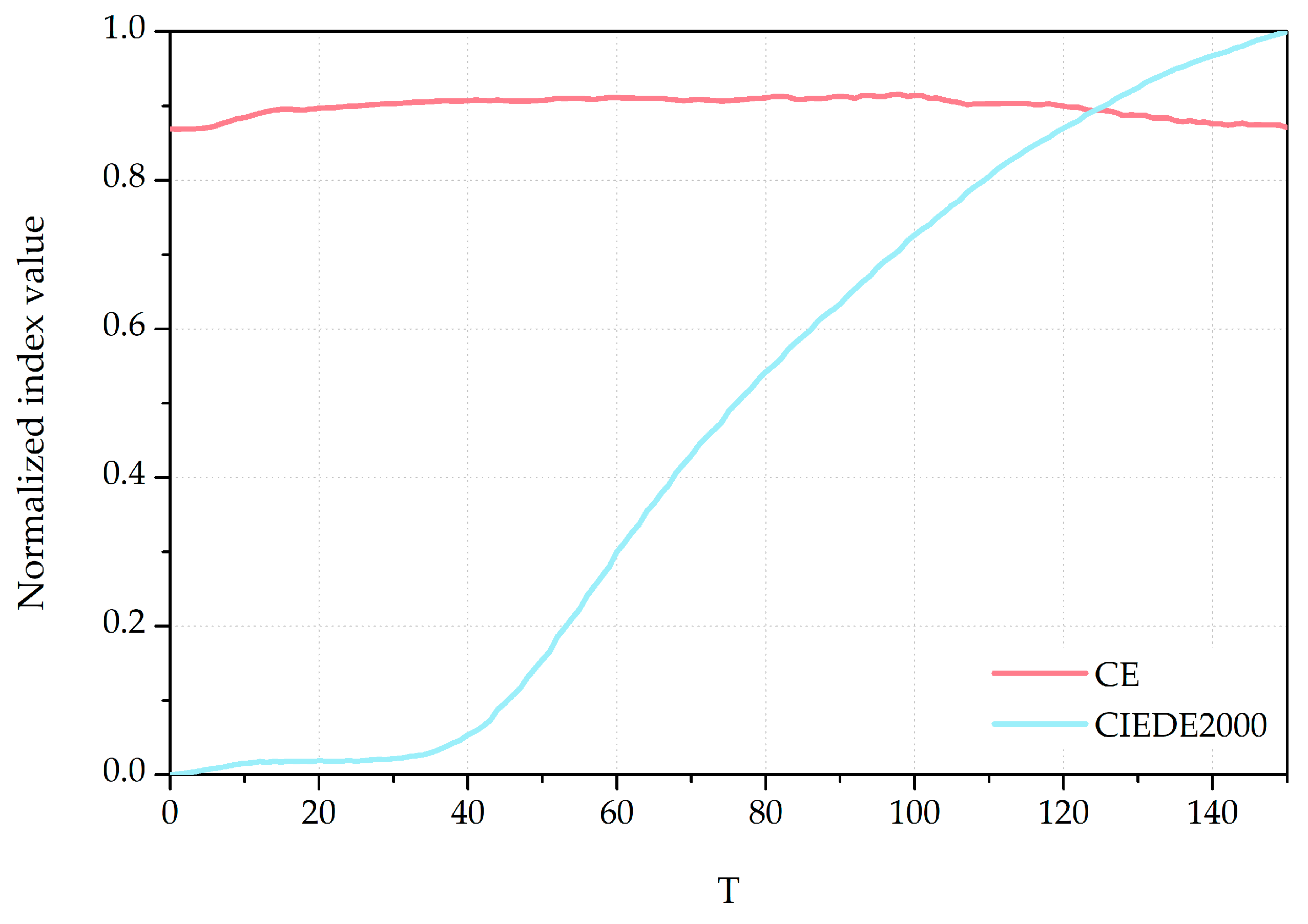
By leveraging the correlation between the lowest value among the R, G, and B color channels of the obscured initial image and the dark-channel prior, the compensation threshold $T$ is established through the application of the contrast energy (CE) and CIEDE2000 metrics. This process enhances the dark-channel image and effectively mitigates the halo effect present in the resulting image.

2.

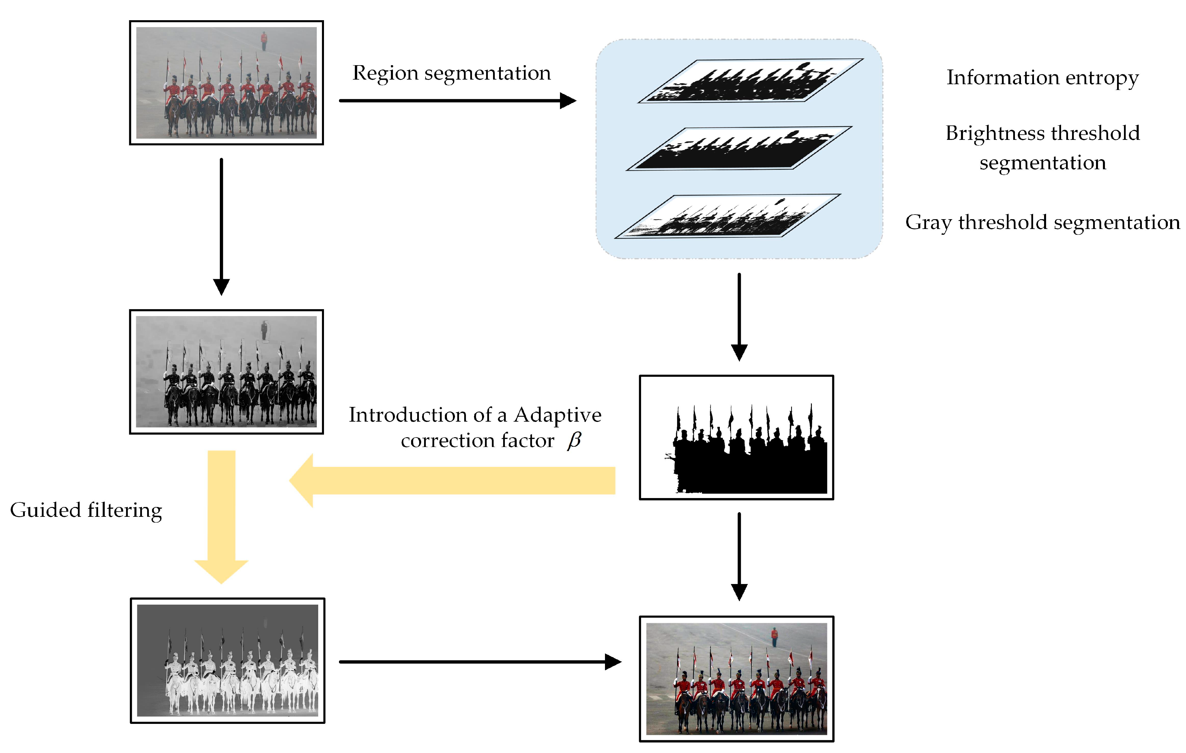
A novel bright-field region-segmentation algorithm is proposed that initially segments the bright-field region based on three prior conditions to determine the baseline of the target area. Subsequently, region growing is employed to further refine the bright-field region.

3.

Introducing an adaptive adjustment factor $\beta$ to optimize the transmittance mapping effectively addresses the potential color distortion issues that may arise in the process of dehazing bright-field regions.

2. DCP Defogging Algorithm and Background

2.1. Atmospheric Scattering Model

In foggy scenes, image quality is degraded due to particles in the atmosphere absorbing and scattering light. In the field of image defogging, Narasimhan et al. [24] proposed an atmospheric scattering model to describe this process as follows:

$$I\left(x\right)=J\left(x\right)t\left(x\right)+A\left(1-t\left(x\right)\right),$$

(1)

where $I\left(x\right)$ represents the degraded foggy image, $J\left(x\right)$ represents the fog-free image to be restored, $A$ is the atmospheric light-intensity value at infinity, and $t\left(x\right)$ is the transmittance of the medium. If $A$ and $t\left(x\right)$ are known, the defogged image $J\left(x\right)$ can be obtained.

2.2. Dark-Channel Prior Defogging

The main idea in [11] is that, in the non-sky local area of most fog-free images, there are always some pixels that meet the condition where the value of at least one color channel is very low and close to zero.

$$J^{\mathrm{d}\mathrm{a}\mathrm{r}\mathrm{k}}\left(x\right)=\underset{y\in \Omega \left(x\right)}{\min }\left(\underset{c\in \left\{r,g,b\right\}}{\min }{J}^c\left(y\right)\right)\to 0,$$

(2)

where $J^{dark}\left(x\right)$ represents the dark-channel image and the value of $c$ channel at $y$ pixel in the $J^c$ fog-free image, and $c\in \left\{R,G,B\right\}$, $\Omega \left(x\right)$ represents the local filtering window centered on $x$ pixel. The atmospheric light is assumed to be known and positive. Equations (1) and (2) can be combined to obtain the transmittance value as follows.

$$t\left(x\right)=1-\omega \underset{y\in \Omega \left(x\right)}{\mathrm{m}\mathrm{i}\mathrm{n}}\left(\underset{\mathit{cϵ}\left\{r,g,b\right\}}{\min }{\displaystyle \frac{I^c\left(y\right)}{A^c}}\right).$$

(3)

To enhance the defogging effect more naturally, a constant coefficient $\omega$ (0 < $\omega$ < 1) is typically added to Equation (3). Generally, $\omega =0.95$. Because the dark-channel graph is compensated in this paper (see Section 3.1), $\omega$ is 0.85.

2.3. Guided Filter

The guiding filter [12] is derived from a local linear model. The filtering output $q$ is calculated by considering the guiding image $I$, which is expressed as the guiding filter by a mathematical formula. The filtering output at pixel $i$ is expressed as

$$q_i={\sum }_j{W}_{ij}\left(I\right)p_j,$$

(4)

where $W_{ij}$ is the filter kernel function, and both $i$ and $j$ denote pixel indices. The filter can be assumed to be a linear model between the guided image $I$ and the filtered output $q$ that can be expressed as

$$q_i=a_k{I}_i+b_k,\forall i\in {\omega }_k,$$

(5)

where ${\omega }_k$ is the local filtering window centered on pixel $k$. The coefficients of linearity $\left(a_k,b_k\right)$ are constant in ${\omega }_k$. The output image $q$ has a gradient correlation with the input image $I$. To reduce the disparity between the input and output images, the goal is to identify the lowest value of the cost function:

$$E\left(a_k,b_k\right)={\sum }_{i\in {\omega }_k}\left({\left(a_k{I}_i+b_k-p_i\right)}^2+ϵa_k^2\right),$$

(6)

where $ϵ$ is the regularization parameter used to prevent $a_k$ from becoming too large. The linear relationship can be fitted using the least-squares method, and the optimal solution of $\left(a_k,b_k\right)$ is obtained as follows:

$$a_k={\displaystyle \frac{\frac{1}{\left|\omega \right|}\sum _{i\in {\omega }_k}{I}_i{p}_i-{\mu }_k{\overline{p}}_k}{{\sigma }_k^2+ϵ}},$$

(7)

$$b_k={\overline{p}}_k-a_k{\mu }_k,$$

(8)

where ${\mu }_k$ and ${\sigma }_k^2$ represent the mean and variance of the guide image $I$ in the local window ${\omega }_k$, respectively, and $\left|\omega \right|$ is the number of pixels in ${\omega }_k$. ${\overline{p}}_k={\displaystyle \frac{1}{\left|\omega \right|}}\sum _{i\in {\omega }_k}{p}_i$ is the average value within ${\omega }_k$.

3. Proposed Algorithm

It is easy to cause a halo effect when using the DCP method. An adaptive image-defogging algorithm based on bright-field region detection (ADBD) is proposed in this paper. Because the dark-channel value of an image is related to the scene’s depth information, this paper compensates the dark-channel map by using the relationship between the minimum RGB three-channel value and the initial dark-channel value of the original foggy image to mitigate the impact of depth-of-field changes. However, for foggy images with large bright-field areas, merely optimizing the dark-channel map cannot resolve the issue of noticeable color bias. Therefore, this paper proposes a new segmentation algorithm for bright-field regions based on information entropy and the thresholds of gray and brightness. The region-growth algorithm is then used for the detailed segmentation of the bright-field region. Finally, an adaptive correction factor is introduced to determine the lower limit of the secondary transmittance, and a nonlinear balance operation is applied to map the transmittance, thereby enhancing the overall brightness of the defogged image. The process flow is illustrated in Figure 1. Each part of the proposed algorithm is discussed in detail below.

3.1. Improved Dark-Channel Image

Based on the concept of the dark-channel prior, the process of calculating the dark channel involves two main steps. The first step is to identify the minimum value (referred to as MC) among the RGB channels. The second step involves selecting a filter window centered around each pixel to determine the minimum value within that window as the dark-channel value for the pixel at the center.

As depicted in Figure 2, the filtering process of the local filter kernel is illustrated in regions where the depth of field exhibits little variation and where the depth of field changes abruptly. The red box represents the neighborhood window selected by the central pixel, and the red solid rectangle represents the central pixel of the local window. The $A$ side has a smaller dark-channel value, while the $B$ side has a larger dark-channel value. If all the pixels in the entire window fall within the smooth region of the actual dark-channel value (either in area $A$ or $B$), the dark-channel value will show a smaller change after the minimum filtering process. If the filtering window is positioned in the $C$ region, the two regions will be adjacent to each other, leading to the formation of a boundary edge band. When the window contains pixels in an area with a small dark-channel value, the dark-channel value of the central pixel of the window is reduced by the surrounding pixels. This causes the dark-channel value of the filtered pixel to be lower than its true value, and the same region value will represent the transmittance of various depths in the scene. As a result, the connection between different depths of field in the image will not be smooth, resulting in a halo effect at the edges. The larger the filtering radius, the more pronounced the multiple depth-of-field information in the window area, and the stronger the halo effect.

This paper introduces a new concept aimed at enhancing the process of acquiring dark-channel images. We propose using the absolute value of the difference between the original dark-channel image and the MC as a criterion to determine if compensations are needed for the original dark-channel image. If the difference is greater than a certain threshold $T$, it is determined that the neighborhood window pixel has a different depth of field from the central pixel. In this case, the MC is used to replace the dark primary color pixel by pixel. Otherwise, the initial dark-channel image is retained.

The improved dark-channel image acquisition steps are as follows:

4.

According to the dark-channel prior theory, the size of $\Omega \left(x\right)$ is $15\times 15$ pixels, and the initial dark-channel image $I^{\mathrm{d}\mathrm{a}\mathrm{r}\mathrm{k}}$ is obtained:

$$I^{\mathrm{d}\mathrm{a}\mathrm{r}\mathrm{k}}=\underset{y\in \Omega \left(x\right)}{\min }\left(\underset{c\in \left\{r,g,b\right\}}{\min }{I}^c\left(y\right)\right)$$

(9)

5.

Obtain the MC:

$$I_{\mathrm{m}\mathrm{i}\mathrm{n}}=\underset{c\in \left\{r,g,b\right\}}{\min }{I}^c$$

(10)

6.

Calculate the absolute value of the difference between the two:

$$k=\left|I_{\mathrm{m}\mathrm{i}\mathrm{n}}-I^{\mathrm{d}\mathrm{a}\mathrm{r}\mathrm{k}}\right|$$

(11)

7.

Screening: When the difference $k$ is greater than $T$, it is considered that the central pixel and its neighborhood are in different depth-of-field ranges. The MC is used to replace and correct pixels of image $I^{\mathrm{d}\mathrm{a}\mathrm{r}\mathrm{k}}$, reducing the impact of changes in the depth of field at the edges.

$${I^{\mathrm{d}\mathrm{a}\mathrm{r}\mathrm{k}}}^{\mathrm{’}}\left(i,j\right)=\left\{\begin{array}{c}{I}_{\mathrm{m}\mathrm{i}\mathrm{n}}\left(i,j\right), k>T\\ I^{\mathrm{d}\mathrm{a}\mathrm{r}\mathrm{k}}\left(i,j\right), k<T\end{array}\right.$$

(12)

8.

Introduce tolerance $T_0$: $T_0$ = 5. In the dark-channel image obtained in the first step, if the gray value of a pixel falls within the tolerance range of $\left|k-T\right|<T_0$, that pixel and the pixels to its left and right are adjusted by the central pixel’s MC.

$$\left.\begin{array}{c}{I^{\mathrm{d}\mathrm{a}\mathrm{r}\mathrm{k}}}^{\prime }\left(i,j+1\right)\\ {I^{\mathrm{d}\mathrm{a}\mathrm{r}\mathrm{k}}}^{\prime }\left(i,j-1\right)\end{array}\right\}=I_{\mathrm{m}\mathrm{i}\mathrm{n}}\left(i,j\right),\left|k-T\right|<T_0$$

(13)

3.2. Determination of Threshold

The size of the threshold $T$ significantly impacts the performance of the algorithm. An appropriate threshold $T$ should ensure that the defogged image remains undistorted and free of halo effects. This requires the transmittance to retain sufficient and accurate depth-of-field information. When $T=0$, there is a difference between the initial dark-channel value and the minimum value of the three RGB color channels. All pixels are replaced by the MC to calculate the transmittance image. Although this can avoid the halo effect, it can easily lead to image supersaturation and an overall dimness in brightness. Detailed information may be lost depending on the color of the original foggy image, as a result of changes in the depth of field, or due to other factors.

Therefore, this paper conducts a statistical analysis of numerous foggy images prone to producing halo effects and determines that the maximum value of the difference $k$ is 150. The difference is calculated for $T=0$ and the transmittance image obtained using the initial dark channel $\left(15\times 15\right)$. A binarization operation is then performed to identify areas prone to halo effects or bright fields. Subsequently, $T$ is incremented in steps of 1 within the range of 0 to 150. For each $T$ value, the color difference between the fog-free image recovered in the difference region is calculated using the CIEDE2000 [25] standard. Simultaneously, it is considered that compensating the dark-channel value of certain pixel points significantly impacts the color of the recovered image. Therefore, the evaluation function contrast energy (CE) [26], which characterizes the color, is adopted as the evaluation index of the defogged image to further clarify the optimal value of $T$. The normalized mean values of CE and CIEDE2000 for multiple images are depicted in Figure 3.

As shown in Figure 3, the transmittance image is more accurate in the difference region when $T$ ranges from 0 to 50, showing a more gradual change and higher precision in the transmittance mapping. When $T$ exceeds 50, the CIEDE2000 indicator shows a dramatic increase, indicating that edge information in the transmittance map becomes incomplete, leading to color shifts in the recovered colors at the image edges. According to Section 3.1, the dark-channel prior theory applies to image pixel neighborhoods rather than individual pixels. Therefore, the $T$ value should take a larger value while preserving enough depth-of-field information to prevent the overcompensation of dark primary colors.

To validate the reasonableness of $T\in \left[\mathrm{35,45}\right]$, the foggy images prone to the halo effect were defogged. Figure 4 and Figure 5 show the restored image and the transmittance image at $T=0$, $T=40,$ $T=100$, and $T=150.$ When $T$ is set between 35 and 45, the transmittance is estimated more accurately, with detailed information remaining largely consistent with that of $T=0$. The color is realistic and natural, effectively improving the halo phenomenon. However, there is still an issue with the smoothness of the color transitions in some regions. In addition, if a foggy image contains large bright-field areas, simply compensating the dark-channel image is insufficient. It is also necessary to segment the bright-field areas and optimize the transmittance (see Section 3.3 and Section 3.4).

3.3. Bright-Field Region Segmentation

The bright-field region-segmentation method proposed in this paper satisfies three prior conditions based on the bright-field areas, such as the sky and white objects in the foggy image. The target region is segmented based on three conditions. There is a uniform distribution of gray level in the pixels within the image. The dark-channel value of the pixels in this region tends to be 1, and the gray values and brightness of the pixels in the target area are relatively high.

In contrast to previous studies, the experiment in this paper focuses on utilizing the $Y$ channel of the YCbCr color space of the foggy image to preserve additional image details. Firstly, the foggy image is transformed into the YCbCr color space. To extract the edge contour gradient information of the whole image, the Sobel operator is used to calculate the gradient value of the $Y$ component in the x and y directions, and then the edge gradient values are normalized. The horizontal (x) direction filtering kernel of the Sobel operator $M$ is

$$M=\left[\begin{array}{ccc}-1& 0& 1\\ -2& 0& 2\\ -1& 0& 1\end{array}\right],$$

(14)

in the y direction (Equation (14)). Convolve the operator filter kernel with the Y component, where $G_x$ and $G_y$ represent the horizontal- and vertical-edge gradients, respectively. The edge gradients are calculated as $G=\sqrt{\left({G_x}^2+{G_y}^2\right)}$. Image entropy (IE) [27] is used to segment the bright-field regions. The entropy value reflects the amount of information in the image. Here, we define IE as $E_i$. The smaller the entropy value, the less information in the image and the more uniform the distribution of gray level. The definition of IE is as follows:

$$E_i=-\sum _v{p}_v{log}_2\left(p_v\right),$$

(15)

where $v$ is the gray level and $p_v$ is the probability associated with $v$. Secondly, according to the gradient image, the information entropy of $15 \times 15$ pixels in the local window is calculated. Due to the minimal changes in the gradient within the bright-field region, $E_i$ tends to zero; then, obtain the dark-channel image of the foggy image ($\Omega \left(x\right)=15 \times 15$ pixels) and set the brightness threshold $T_1$. If the dark-channel value is greater than $T_1$, it may indicate the bright-field region. Here, $T_1=\min \left(\alpha ,0.75\right)$ because the overall brightness of some foggy images is dark, and after normalization, the dark-channel value of the bright-field areas such as the sky is close to 0.5. Therefore, a correction factor $\alpha$ was introduced after multiple experiments on foggy images containing clear field areas. Ultimately, $\alpha$ was determined to be the maximum value in the normalized dark-channel image minus 0.1. Finally, the sky serves as a typical representation of the bright-field region. In foggy images including sky, the proportion of the sky region is generally greater than 5% [28]. The grayscale histogram reflects the frequency of occurrence of a certain grayscale in the image, with the target region accounting for a relatively large proportion (mostly concentrated in the higher gray levels). Therefore, the grayscale threshold $T_2$ is defined as

$$T_2=r_{max}-30,$$

(16)

where $r_{max}$ represents the grayscale with the highest probability in foggy images.

The region that satisfies the above conditions is defined as the initial bright-field region. Subsequently, the bright-field area is refined.

Firstly, skeletonize the field region and identify the feature points (endpoints and turning points). Then, these feature points are used as growth factors for region expansion to realize the growth of the region. Check if the recently separated target area includes all the feature points, and repeat the process until all the points are within the target region. Finally, apply a morphological opening operation to the image to eliminate incorrectly identified connected regions in the non-bright-field area. Figure 6 illustrates the overall segmentation process of the bright-field region.

3.4. Transmission-Adaptive Optimization

In this paper, the top 0.1% of the brightest pixels from the initial dark-channel image are selected, and their mean value in the original image is considered as the atmospheric light value. Incorporating ${I^{\mathrm{d}\mathrm{a}\mathrm{r}\mathrm{k}}}^{\prime }$ and $A$ into Equation (3) allows for the calculation of coarse transmittance. This section introduces a primarily adaptive optimization method for transmittance.

In the enhanced dark-channel image, although the depth of field at the edge is more precise, a “pseudo edge” may appear near the threshold. In image defogging, guide filtering is generally employed to refine the transmittance image. The grayscale image of the fog serves as the reference image, while the coarse transmittance image is used as the input image. This technique improves the image’s quality while preserving the integrity of its edge details.

In bright areas, such as the sky, it does not meet the prior condition of the dark channel. That is, the values of the three RGB color channels are not close to zero and are greater than zero after the minimum filtering in the pixel neighborhood. Thus,

$$t^{\mathrm{b}\mathrm{r}\mathrm{i}\mathrm{g}\mathrm{h}\mathrm{t}}\left(x\right)={\displaystyle \frac{1-\underset{y\in \Omega \left(x\right)}{\mathrm{m}\mathrm{i}\mathrm{n}}\left(\underset{\mathit{cϵ}\left\{r,g,b\right\}}{\min }\frac{I^c\left(y\right)}{A^c}\right)}{1-\underset{y\in \Omega \left(x\right)}{\mathrm{m}\mathrm{i}\mathrm{n}}\left(\underset{\mathit{cϵ}\left\{r,g,b\right\}}{\min }\frac{J^c\left(y\right)}{A^c}\right)}}>1-\underset{y\in \Omega \left(x\right)}{\mathrm{m}\mathrm{i}\mathrm{n}}\left(\underset{\mathit{cϵ}\left\{r,g,b\right\}}{\min }{\displaystyle \frac{I^c\left(y\right)}{A^c}}\right).$$

(17)

The actual transmittance in the bright-field region is higher than that predicted by the dark-channel prior theory in this area. Additionally, the smaller $1-\underset{y\in \Omega \left(x\right)}{\mathrm{m}\mathrm{i}\mathrm{n}}\left(\underset{cϵ\left\{r,g,b\right\}}{\mathrm{m}\mathrm{i}\mathrm{n}}\left({\displaystyle \frac{J^c\left(y\right)}{A^c}}\right)\right)$ is, the larger $t^{\mathrm{b}\mathrm{r}\mathrm{i}\mathrm{g}\mathrm{h}\mathrm{t}}\left(x\right)$ becomes. Therefore, when restoring the defogged image in the segmented bright-field region, it is necessary to use a higher transmittance value. This value is referred to as the second lower limit of transmittance ${t_0}^{\prime }$, and it is crucial for achieving defogging in the bright-field region. In some foggy images, the bright-field region exhibits a higher average brightness, leading to a significant deviation when calculating transmittance using the dark-channel prior. It is typically lower. If the lower bound value is fixed, the color shift will still occur in some bright-field regions. In other words, the transmittance of the highlighted region is not adequately compensated, and the fixed lower limit value does not effect it.

Grayscale values characterize luminance. This study attempts to use the mean grayscale value of the segmented sky region as a factor to adjust the lower limit of transmittance in the sky region. $\beta$ is defined as follows:

$$\beta =0.2+0.2\ast {\displaystyle \frac{I_{ds}}{255}},$$

(18)

$${t_0}^{\mathrm{\prime }}=\mathrm{m}\mathrm{a}\mathrm{x}\left(\beta ,0.35\right),$$

(19)

where $I_{ds}$ is the average value of the gray level in the bright-field region (Section 3.3).

Considering the scarcity of real foggy sky datasets, this paper uses the SOTS outdoor synthetic dataset containing sky regions. Equation (19) and a fixed lower limit of 0.35 were applied separately for defogging, and the results were compared with real clear images. The original clear image had IE and natural image quality estimation (NIQE) metrics of 7.40 and 2.94, respectively. Using Equation (19), the obtained metrics were 7.25 and 3.02, closely matching the original values. This strongly proves the effectiveness of the $\beta$ setting, indicating that the restored image retains more detail without noticeable color bias. According to experience, for non-bright-field regions, it is also necessary to set the lower limit of transmittance, which is called the first lower limit of transmittance $t_0$, and it is set at 0.1. A nonlinear balance is used to map the transmittance, effectively preserving the information of the original image while compressing the dynamic range. This process enhances the contrast and quality of the image.

After determining the atmospheric light and transmittance, the defogged image is restored using the atmospheric scattering model. If the bright-field region identified in Section 3.3 exceeds 5% of the total image, the second lower limit of transmittance is applied. Otherwise, the first lower limit is used. The final defogged image is represented as follows:

$$J\left(x\right)={\displaystyle \frac{I\left(x\right)-A}{\mathrm{m}\mathrm{a}\mathrm{x}\left(t\left(x\right),t\right)}}+A,$$

(20)

where $t$ is the unified representation of the first and second lower-transmittance bounds.

4. Experiment and Discussion

This section compares the proposed method with several other typical algorithms, using subjective and objective evaluation metrics to analyze and assess the outcomes of defogging. In addition to the PSD algorithm, all the tests and experiments in this paper were performed on a computer configured with Inter(R) Core (TM) I7-12700 2.10 GHz CPU in the Matlab R2018b environment.

4.1. Dataset

The RESIDE [29] dataset includes synthetic and real-world images with ambiguity and provides evaluation criteria for various dehazing algorithms. Specifically, the real-world image dataset used in this article was partly manually collected from the internet, including from the HSTS dataset in RESIDE, and partly captured using a Sony DSC-WX700 camera. The synthetic dataset used SOTS, which replicates the same process as the training data to synthesize blurred images.

4.2. Image Quality Evaluation Method

The evaluation of the haze-removal algorithm was performed both subjectively and objectively. The subjective evaluation included analysis of the degree of haze removal, detail retention, edge sharpness, the naturalness of color restoration, and the presence of color bias, artefacts, and halos. For the objective evaluation, structural similarity (SSIM), peak signal-to-noise ratio (PSNR), natural image quality estimation (NIQE) [30], and saturated pixel ratio (σ) [31] quantitative metrics were used to measure haze-removal performance. These aspects collectively determined the overall quality of the defogging results.

4.3. Result Analysis

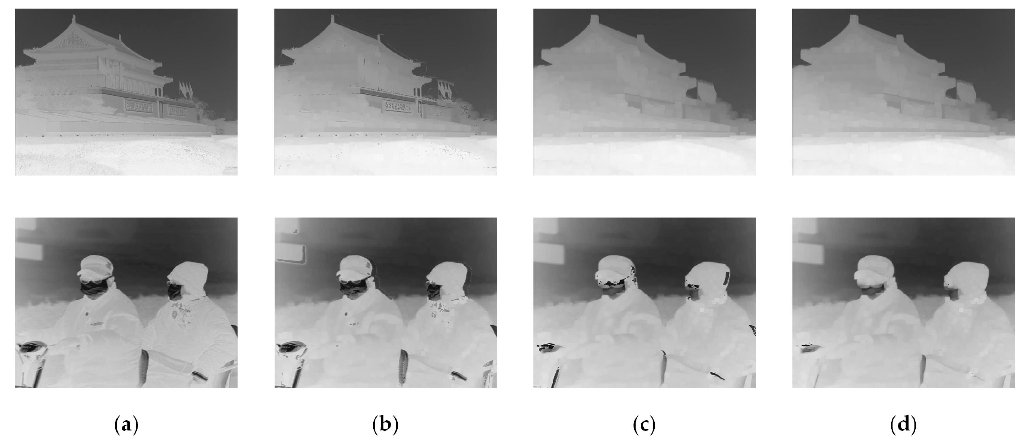
4.3.1. Comparison with DCP Algorithm

To verify the algorithm’s effectiveness in reducing halo effects and color distortion, the defogged image was compared to the DCP algorithm using a guided filter.

In Figure 7c, the DCP algorithm produces distinct halos where the depth of field changes abruptly, especially in bright areas like the sky and road, causing significant color distortion. In contrast, the ADBD algorithm (Figure 7e) improves color accuracy in these areas by segmenting regions, adaptively optimizing transmittance, and performing nonlinear balancing operations. Transmittance images from both algorithms are shown in Figure 7b,d. The ADBD algorithm yields more accurate transmittance images, resulting in a more natural scene, as seen in the flower basket, sky, and clear edges of the Tian’an City Gate. This adaptive process preserves edge information and better aligns the colors of the defogged image with what humans perceive.

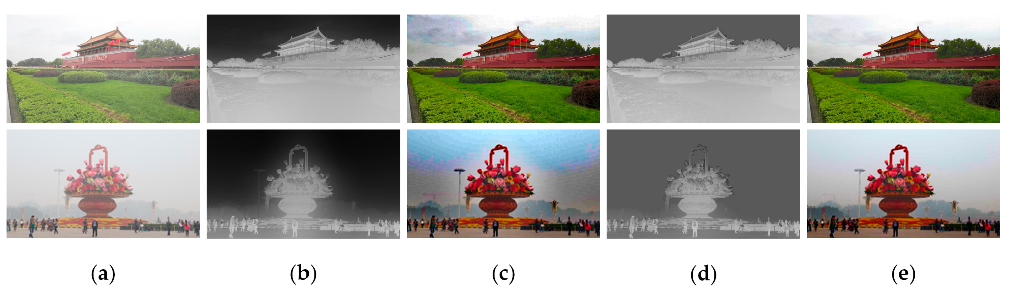
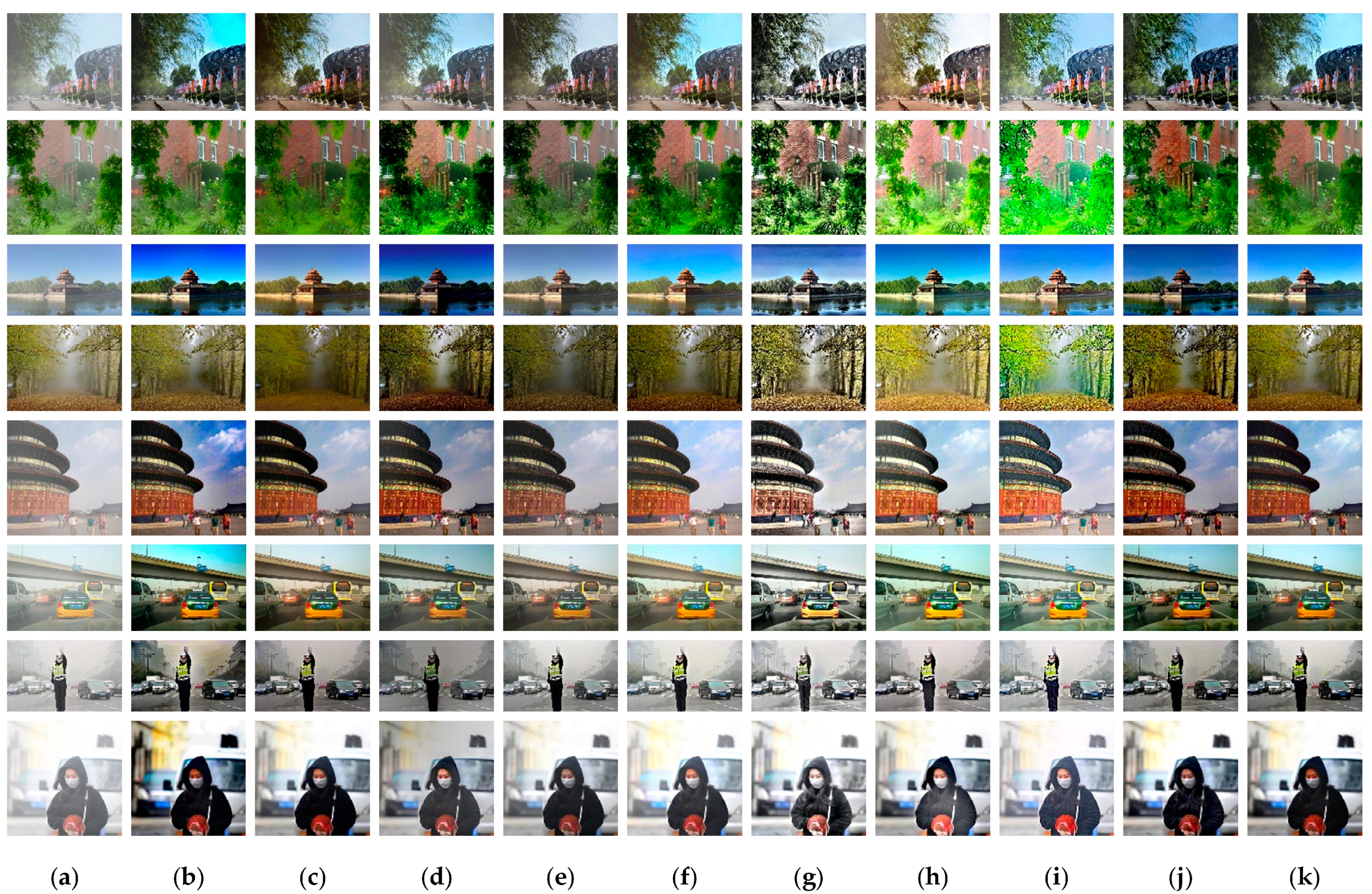
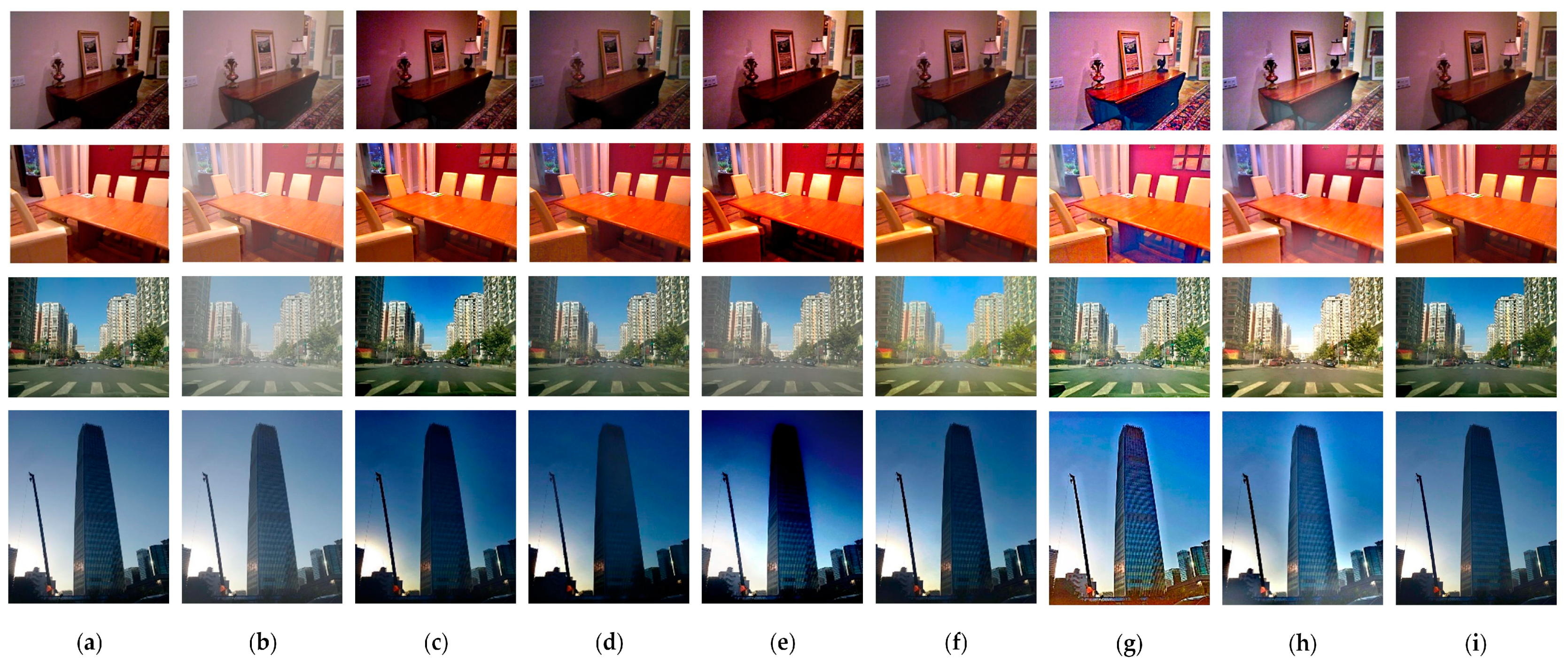
4.3.2. Comparison with Other Methods

Using DCP [12], CAP [13], DEFADE [32], ICAP [33], OTM-AAL [34], RADE [35], IDE [36], PSD [37], CEEF [38], and the methods proposed in this paper, defogging comparisons were conducted. Figure 8 displays the comparison results of the nine dehazing algorithms using the RESIDE and HSTS datasets.

The defogged image produced by the RADE algorithm exhibits significant halo artifacts in regions with sharp changes in depth of field. The leaves in the image show significant color distortion, and the overall tone is grayish white. The results obtained by the DCP algorithm have halos. For example, the transition between the policewoman and the sky background is not natural enough. There is still a slight fog present where the leaves meet the red wall, and the CEEF algorithm experiences a similar issue. The defogged images obtained by the CAP, DEFADE, ICAP, OTM-AAL, and ADBD algorithms show no apparent halo phenomenon. In contrast, OTM-AAL, IDE, and the algorithm presented in this paper have higher color fidelity and brightness. The IDE and PSD algorithms can enhance the brightness of defogged images and preserve details more completely; however, some areas may become overexposed, resulting in color distortion and an unnatural defogging effect. For the overall effect, the color accuracy in CAP is improved, but some areas show a loss of detail. The brightness of DEFADE is dim and it has the problem of over-enhancement. For example, the details at the junction of the lake and the building are lost and appear almost black. In contrast, the images restored by the proposed algorithm appear more natural. For fogged images with sky and other bright areas, the results of ADBD are comparable to DCP in nearby regions and outperform OTM-AAL in distant regions. For example, the sky regions in images 1, 5, and 6 do not exhibit significant color distortion; in image 4, there is less residual haze in the deep forest area, and detail information is appropriately enhanced. These results demonstrate the algorithm’s strengths in color restoration and detail preservation. Furthermore, for the eight images presented in Figure 8, several methods are evaluated using four evaluation indicators: SSIM, PSNR, NIQE, and σ, as shown in

Table 1. Quantitative comparison of defogging images obtained by ten comparison methods.

Foggy Image	DCP			CAP			DEFADE			ICAP			OTM-AAL
	ssim	psnr	NI QE	ssim	psnr	NI QE	ssim	psnr	NI QE	ssim	psnr	NI QE	ssim	psnr	NI QE
1	0.79	12.01	3.19	0.81	11.86	3.00	0.91	17.35	3.10	0.84	13.49	3.03	0.88	15.00	2.66
2	0.95	20.07	3.64	0.85	15.53	3.29	0.78	15.77	3.72	0.90	17.79	3.73	0.89	16.21	3.12
3	0.77	10.97	3.68	0.88	14.62	3.85	0.66	9.25	3.74	0.87	16.17	4.05	0.85	16.28	3.80
4	0.93	17.76	2.62	0.72	12.59	2.81	0.77	12.93	2.55	0.83	12.70	3.52	0.85	13.66	2.47
5	0.75	10.92	2.59	0.82	12.49	2.71	0.83	12.59	2.74	0.88	14.23	2.97	0.90	16.37	2.76
6	0.75	10.08	3.36	0.84	12.05	3.49	0.81	11.24	3.60	0.88	13.42	3.56	0.91	15.93	3.39
7	0.71	13.57	3.19	0.82	19.47	3.38	0.83	11.86	3.35	0.91	16.15	3.95	0.93	20.23	3.95
8	0.64	8.55	5.07	0.81	12.16	5.38	0.87	11.78	5.02	0.87	13.74	5.01	0.93	17.61	5.08
Foggy Image	RADE			IDE			PSD			CEEF			Proposed Method
	ssim	psnr	NI QE	ssim	psnr	NI QE	ssim	psnr	NI QE	ssim	psnr	NI QE	ssim	psnr	NI QE
1	0.57	12.49	4.50	0.81	16.19	3.25	0.74	16.31	4.70	0.66	10.61	3.89	0.88	16.43	2.65
2	0.56	14.50	5.06	0.81	15.10	3.63	0.70	14.28	5.08	0.77	14.00	3.66	0.95	18.81	2.95
3	0.67	13.59	3.12	0.71	14.35	3.45	0.84	16.35	3.94	0.71	10.22	3.74	0.89	16.58	3.54
4	0.59	14.34	2.97	0.72	16.64	2.41	0.70	14.79	2.63	0.72	12.80	2.57	0.93	16.90	2.45
5	0.68	14.56	2.87	0.83	16.02	2.55	0.81	18.69	3.12	0.71	10.63	2.53	0.88	15.82	2.59
6	0.66	13.22	2.89	0.82	13.97	3.10	0.83	18.25	3.04	0.70	9.95	3.15	0.90	13.98	2.92
7	0.80	12.65	3.20	0.89	15.94	4.06	0.86	20.19	3.68	0.76	11.22	4.13	0.88	18.74	3.24
8	0.80	15.39	4.87	0.86	14.03	4.88	0.89	18.72	4.03	0.73	11.19	4.22	0.92	16.89	4.13

and

Table 2. The $\sigma$ of defogging images obtained by ten comparison methods.

Foggy Image	DCP	CAP	DEFADE	ICAP	OTM-AAL	RADE	IDE	PSD	CEEF	Ours
1	0.03	0.00	0.00	0.00	0.00	0.15	0.01	0.10	0.77	0.03
2	0.00	0.00	1.63	0.06	0.01	0.04	0.00	0.34	0.03	0.00
3	0.06	0.00	2.62	0.00	0.00	0.08	0.02	0.02	0.55	0.00
4	0.00	0.00	0.94	0.02	0.01	0.11	0.01	0.99	1.14	0.00
5	0.01	0.02	0.01	0.00	0.00	0.23	0.23	0.02	3.26	0.00
6	0.03	0.00	0.00	0.00	0.00	0.01	0.00	0.00	0.16	0.00
7	1.43	4.84	4.68	0.41	0.09	0.01	1.17	0.69	4.24	0.68
8	1.91	0.23	0.00	0.00	0.00	0.00	0.08	0.00	1.42	0.00

.

The SSIM values obtained using the algorithm in this article are the highest in the second, third, and fourth images, at 0.95, 0.89, and 0.93, respectively. Simultaneously, the restored images also have a high PSNR and strong robustness. In contrast, the overall effect of the defogged images is more natural and the color restoration is more realistic, resulting in the best NIQE value and a lower $\sigma$ score.

To verify the applicability of the algorithm proposed in this paper, an experimental analysis was conducted on the complete SOTS dataset. The algorithm was compared with six other more effective defogging algorithms: DCP, CAP, DEFADE, OTM-AAL, IDE, and PSD. The average SSIM and PSNR results for the SOTS indoor and outdoor datasets are shown in

Table 3. Average SSIM and PSNR values with SOTS dataset (compared to clear images).

Method	Outdoor		Indoor
	ssim	psnr	ssim	psnr
DCP	0.76	11.48	0.72	10.51
CAP	0.74	11.57	0.75	11.25
DEFADE	0.80	12.24	0.77	12.82
OTM-AAL	0.90	15.95	0.89	15.75
IDE	0.85	16.32	0.84	15.23
PSD	0.77	17.20	0.79	17.03
Proposed method	0.88	16.29	0.86	14.96

.

The higher SSIM and PSNR values in the outdoor dataset are due to the improved dark channel, compensating for the inaccurate depth estimation in the dark-channel prior. Figure 9 shows only a few challenging defogging results (including large areas of sky and white objects) from the SOTS dataset. The algorithm presented in this paper has demonstrated outstanding performance in subjective vision, outperforming other algorithms in terms of overall effect and detail preservation. Specifically, the algorithm proposed in this paper is more thorough at dehazing. The results of the PSD algorithm vary significantly across different scenarios, with severe color distortion observed in the first and second indoor images. For the third and fourth images in Figure 9, DCP, CAP, DEFADE, and OTM-AAL are excessively enhanced, leading to various degrees of loss of detailed information in the scene. Slight halos are present with both the PSD and IDE algorithms. In contrast, ADBD achieves a natural transition between the foreground and background with higher color fidelity, aligning more lines with human visual perception, resulting in better defogging quality.

To further verify the effectiveness of the algorithm introduced in this study, the OTM-AAL algorithm with the best performance in Table 3 was selected, and the average processing time was calculated. The experimental subjects comprised the images shown in Figure 8 and Figure 9, totaling 12 images. The sizes were 550 × 468, 440 × 440, 553 × 334, 1024 × 768, 550 × 549, 550 × 413, 900 × 558, 599 × 600, 620 × 460, 620 × 460, 550 × 413, and 550 × 665. The average processing time for OTM-AAL was found to be 42.3480 s, whereas the proposed algorithm recorded a significantly shorter time of 1.8486 s. This notable difference indicates that the proposed algorithm outperforms OTM-AAL in terms of speed and can deliver a superior subjective defogging outcome.

5. Conclusions

In this paper, an adaptive image-defogging algorithm based on bright-field region detection is proposed. The algorithm optimizes transmittance mapping from two aspects: improving dark-channel images and detecting bright-field regions. Compared to existing mainstream algorithms, the ADBD algorithm exhibits excellent SSIM and PSNR indices in both synthetic datasets and real images, and it performs best in the NIQE and $\sigma$ indices. Furthermore, it achieves visually superior results compared to other algorithms. However, the algorithm involves many manually set parameters, and different parameter settings can affect the defogging effect. Future research will focus on two elements:

• Developing defogging algorithms with lower time complexity and higher robustness while maintaining image resolution;
• How traditional algorithms and neural networks can learn from each other to propose new defogging models for the better realization of the defogging task.

References

1. Yang, W.; Wang, W.; Huang, H.; Wang, S.; Liu, J. Sparse Gradient Regularized Deep Retinex Network for Robust Low-Light Image Enhancement. IEEE Trans. Image Process. 2021, 30, 2072–2086. [Google Scholar] [CrossRef]
2. Hu, Q.; Zhang, Y.; Zhu, Y.; Jiang, Y.; Song, M. Single Image Dehazing Algorithm Based on Sky Segmentation and Optimal Transmission Maps. Vis. Comput. 2023, 39, 997–1013. [Google Scholar] [CrossRef]
3. Kapoor, R.; Gupta, R.; Son, L.H.; Kumar, R.; Jha, S. Fog Removal in Images Using Improved Dark Channel Prior and Contrast Limited Adaptive Histogram Equalization. Multimed. Tools Appl. 2019, 78, 23281–23307. [Google Scholar] [CrossRef]
4. Stark, J.A. Adaptive Image Contrast Enhancement Using Generalizations of Histogram Equalization. IEEE Trans. Image Process. 2000, 9, 889–896. [Google Scholar] [CrossRef]
5. Hai, J.; Hao, Y.; Zou, F.; Lin, F.; Han, S. Advanced RetinexNet: A Fully Convolutional Network for Low-Light Image Enhancement. Signal Process. Image Commun. 2023, 112, 116916. [Google Scholar] [CrossRef]
6. Gamini, S.; Kumar, S.S. Homomorphic Filtering for the Image Enhancement Based on Fractional-Order Derivative and Genetic Algorithm. Comput. Electr. Eng. 2023, 106, 108566. [Google Scholar] [CrossRef]
7. Cui, Y.; Zhi, S.; Liu, W.; Deng, J.; Ren, J. An Improved Dark Channel Defogging Algorithm Based on the HSI Colour Space. IET Image Process. 2022, 16, 823–838. [Google Scholar] [CrossRef]
8. Tan, R.T. Visibility in Bad Weather from a Single Image. In Proceedings of the 2008 IEEE Conference on Computer Vision and Pattern Recognition, Anchorage, AK, USA, 23–28 June 2008; pp. 1–8. [Google Scholar]
9. Meng, G.; Wang, Y.; Duan, J.; Xiang, S.; Pan, C. Efficient Image Dehazing with Boundary Constraint and Contextual Regularization. In Proceedings of the 2013 IEEE International Conference on Computer Vision, Sydney, Australia, 1–8 December 2013; pp. 617–624. [Google Scholar]
10. Berman, D.; Treibitz, T.; Avidan, S. Non-Local Image Dehazing. In Proceedings of the 2016 IEEE Conference on Computer Vision and Pattern Recognition (CVPR), Las Vegas, NV, USA, 27–30 June 2016; pp. 1674–1682. [Google Scholar]
11. He, K.; Sun, J.; Tang, X. Single Image Haze Removal Using Dark Channel Prior. In Proceedings of the 2009 IEEE Conference on Computer Vision and Pattern Recognition, Miami, FL, USA, 20–25 June 2009; pp. 1956–1963. [Google Scholar]
12. He, K.; Sun, J.; Tang, X. Guided Image Filtering. IEEE Trans. Pattern Anal. Mach. Intell. 2013, 35, 1397–1409. [Google Scholar] [CrossRef]
13. Zhu, Q.; Mai, J.; Shao, L. A Fast Single Image Haze Removal Algorithm Using Color Attenuation Prior. IEEE Trans. Image Process. 2015, 24, 3522–3533. [Google Scholar] [CrossRef] [PubMed]
14. Chen, Z.; Ou, B.; Tian, Q. An Improved Dark Channel Prior Image Defogging Algorithm Based on Wavelength Compensation. Earth Sci. Inform. 2019, 12, 501–512. [Google Scholar] [CrossRef]
15. Shi, H.; Han, L.; Fang, L.; Dong, H. Improved Color Image Defogging Algorithm Based on Dark Channel Prior. J. Intell. Fuzzy Syst. 2022, 43, 8187–8193. [Google Scholar] [CrossRef]
16. Cai, B.; Xu, X.; Jia, K.; Qing, C.; Tao, D. DehazeNet: An End-to-End System for Single Image Haze Removal. IEEE Trans. Image Process. 2016, 25, 5187–5198. [Google Scholar] [CrossRef]
17. Li, B.; Peng, X.; Wang, Z.; Xu, J.; Feng, D. AOD-Net: All-in-One Dehazing Network. In Proceedings of the 2017 IEEE International Conference on Computer Vision (ICCV), Venice, Italy, 22–29 October 2017; pp. 4780–4788. [Google Scholar]
18. Dong, H.; Pan, J.; Xiang, L.; Hu, Z.; Zhang, X.; Wang, F.; Yang, M.-H. Multi-Scale Boosted Dehazing Network with Dense Feature Fusion. In Proceedings of the 2020 IEEE/CVF Conference on Computer Vision and Pattern Recognition (CVPR), Seattle, WA, USA, 13–19 June 2020; pp. 2154–2164. [Google Scholar]
19. Guo, C.; Yan, Q.; Anwar, S.; Cong, R.; Ren, W.; Li, C. Image Dehazing Transformer with Transmission-Aware 3D Position Embedding. In Proceedings of the 2022 IEEE/CVF Conference on Computer Vision and Pattern Recognition (CVPR), New Orleans, LA, USA, 18–24 June 2022; pp. 5802–5810. [Google Scholar]
20. Yang, Y.; Wang, C.; Liu, R.; Zhang, L.; Guo, X.; Tao, D. Self-Augmented Unpaired Image Dehazing via Density and Depth Decomposition. In Proceedings of the 2022 IEEE/CVF Conference on Computer Vision and Pattern Recognition (CVPR), New Orleans, LA, USA, 18–24 June 2022; pp. 2027–2036. [Google Scholar]
21. Li, L.; Dong, Y.; Ren, W.; Pan, J.; Gao, C.; Sang, N.; Yang, M.-H. Semi-Supervised Image Dehazing. IEEE Trans. Image Process. 2020, 29, 2766–2779. [Google Scholar] [CrossRef]
22. Wu, R.-Q.; Duan, Z.-P.; Guo, C.-L.; Chai, Z.; Li, C. RIDCP: Revitalizing Real Image Dehazing via High-Quality Codebook Priors. In Proceedings of the 2023 IEEE/CVF Conference on Computer Vision and Pattern Recognition (CVPR), Vancouver, BC, Canada, 17–24 June 2023; pp. 22282–22291. [Google Scholar]
23. Zhu, M.; He, B.; Liu, J.; Zhang, L. Dark Channel: The Devil Is in the Details. IEEE Signal Process. Lett. 2019, 26, 981–985. [Google Scholar] [CrossRef]
24. Narasimhan, S.G.; Nayar, S.K. Vision and the Atmosphere. Int. J. Comput. Vis. 2002, 48, 233–254. [Google Scholar] [CrossRef]
25. Pereira, A.; Carvalho, P.; Côrte-Real, L. Boosting Color Similarity Decisions Using the CIEDE2000_PF Metric. Signal Image Video Process. 2022, 16, 1877–1884. [Google Scholar] [CrossRef]
26. Groen, I.I.A.; Ghebreab, S.; Prins, H.; Lamme, V.A.F.; Scholte, H.S. From Image Statistics to Scene Gist: Evoked Neural Activity Reveals Transition from Low-Level Natural Image Structure to Scene Category. J. Neurosci. 2013, 33, 18814–18824. [Google Scholar] [CrossRef]
27. Hayashi, T.; Cimr, D.; Fujita, H.; Cimler, R. Image Entropy Equalization: A Novel Preprocessing Technique for Image Recognition Tasks. Inf. Sci. 2023, 647, 119539. [Google Scholar] [CrossRef]
28. Liu, Y.; Li, H.; Wang, M. Single Image Dehazing via Large Sky Region Segmentation and Multiscale Opening Dark Channel Model. IEEE Access 2017, 5, 8890–8903. [Google Scholar] [CrossRef]
29. Li, B.; Ren, W.; Fu, D.; Tao, D.; Feng, D.; Zeng, W.; Wang, Z. Benchmarking Single-Image Dehazing and Beyond. IEEE Trans. Image Process. 2019, 28, 492–505. [Google Scholar] [CrossRef]
30. Mittal, A.; Soundararajan, R.; Bovik, A.C. Making a “Completely Blind” Image Quality Analyzer. IEEE Signal Process. Lett. 2013, 20, 209–212. [Google Scholar] [CrossRef]
31. Hautière, N.; Tarel, J.-P.; Aubert, D.; Dumont, É. Blind contrast enhancement assessment by gradient ratioing at visible edges. Image Anal. Ster. 2011, 27, 87–95. [Google Scholar] [CrossRef]
32. Choi, L.K.; You, J.; Bovik, A.C. Referenceless Prediction of Perceptual Fog Density and Perceptual Image Defogging. IEEE Trans. Image Process. 2015, 24, 3888–3901. [Google Scholar] [CrossRef]
33. Ngo, D.; Lee, G.-D.; Kang, B. Improved Color Attenuation Prior for Single-Image Haze Removal. Appl. Sci. 2019, 9, 4011. [Google Scholar] [CrossRef]
34. Ngo, D.; Lee, S.; Kang, B. Robust Single-Image Haze Removal Using Optimal Transmission Map and Adaptive Atmospheric Light. Remote Sens. 2020, 12, 2233. [Google Scholar] [CrossRef]
35. Li, Z.; Zheng, X.; Bhanu, B.; Long, S.; Zhang, Q.; Huang, Z. Fast Region-Adaptive Defogging and Enhancement for Outdoor Images Containing Sky. In Proceedings of the 2020 25th International Conference on Pattern Recognition (ICPR), Milan, Italy, 10–15 January 2021; pp. 8267–8274. [Google Scholar]
36. Ju, M.; Ding, C.; Ren, W.; Yang, Y.; Zhang, D.; Guo, Y.J. IDE: Image Dehazing and Exposure Using an Enhanced Atmospheric Scattering Model. IEEE Trans. Image Process. 2021, 30, 2180–2192. [Google Scholar] [CrossRef]
37. Chen, Z.; Wang, Y.; Yang, Y.; Liu, D. PSD: Principled Synthetic-to-Real Dehazing Guided by Physical Priors. In Proceedings of the 2021 IEEE/CVF Conference on Computer Vision and Pattern Recognition (CVPR), Nashville, TN, USA, 19–25 June 2021; pp. 7176–7185. [Google Scholar]
38. Nie, J.; Wu, H.; Yao, S. Image Defogging Based on Joint Contrast Enhancement and Multi-Scale Fusion. In Proceedings of the 2023 IEEE 3rd International Conference on Power, Electronics and Computer Applications (ICPECA), Shenyang, China, 29–31 January 2023; pp. 1–7. [Google Scholar]
Figure 1. Flowchart of the proposed algorithm.
Photonics 11 00718 g001
Figure 2. Schematic of dark-channel filtering: (a) smooth region filtering of dark-channel value; (b) edge filtering of dark-channel value variation.
Photonics 11 00718 g002
Figure 3. The mean values of CE and CEIEDE2000 at different T values.
Photonics 11 00718 g003
Figure 4. Defogging results with different T values: (a) fog image; (b) result with T = 0 ; (c) result with T = 40 ; (d) result with T = 100 ; (e) result with T   =   150 .
Photonics 11 00718 g004
Figure 5. Contrast of transmittance images: (a) result with T = 0 ; (b) result with T = 40 ; (c) result with T = 100 ; (d) result with T = 150 .
Photonics 11 00718 g005
Figure 6. Bright-field region-segmentation process: (a) original foggy image; (b) local information entropy processing; (c) T 1 segmentation; (d) T 2 segmentation; (e) initial bright-field region; (f) morphological refinement of bright-field region.
Photonics 11 00718 g006
Figure 7. Comparison with the defogging results of DCP: (a) original foggy images; (b) transmittance diagrams of DCP; (c) results of DCP; (d) transmittance diagrams of the proposed method; (e) results of the proposed method.
Photonics 11 00718 g007
Figure 8. Comparison of images obtained by different algorithms: (a) original foggy images; (b) DCP with GF; (c) CAP; (d) DEFADE; (e) ICAP; (f) OTM-AAL; (g) RADE; (h) IDE; (i) PSD; (j) CEEF; (k) proposed method.
Photonics 11 00718 g008
Figure 9. Comparison of partial defogging results with SOTS dataset: (a) original clear images; (b) synthetic foggy images; (c) DCP with GF; (d) CAP; (e) DEFADE; (f) OTM-AAL; (g) PSD; (h) IDE; (i) proposed method.
Photonics 11 00718 g009