Abstract
Light Detection and Ranging (LiDAR) sensors can precisely determine object distances using the pulsed time of flight (TOF) or amplitude-modulated continuous wave (AMCW) TOF methods and velocity using the frequency-modulated continuous wave (FMCW) approach. In this paper, we focus on modelling and analysing the reflection of vector beams (VBs) and vector vortex beams (VVBs) for optical sensing in LiDAR applications. Unlike traditional TOF and FMCW methods, this novel approach uses VBs and VVBs as detection signals to measure the orientation of reflecting surfaces. A key component of this sensing scheme is understanding the relationship between the characteristics of the reflected optical fields and the orientation of the reflecting surface. To this end, we develop a computational model for the reflection of VBs and VVBs. This model allows us to investigate critical aspects of the reflected field, such as intensity distribution, intensity centroid offset, reflectance, and the variation of the intensity range measured along the azimuthal direction. By thoroughly analysing these characteristics, we aim to enhance the functionality of LiDAR sensors in detecting the orientation of reflecting surfaces.
1. Introduction
LiDAR is a method used to determine distances by directing a laser at an object or surface and measuring the time it takes for the reflected light to return to the receiver, and it can be categorised into two schemes: pulsed time of flight (TOF) [1,2] and amplitude-modulated continuous wave (AMCW) TOF [3,4]. Additionally, another sensing scheme called frequency-modulated continuous wave (FMCW) is also commonly used in LiDAR. By analysing the beat signal between the emitted and reflected frequency-modulated optical signals, both the distance and the velocity of a moving object can be measured [5,6]. LiDAR finds extensive applications across various scenarios: terrestrial and mobile scenarios [7], environmental monitoring and conservation [8], archaeology and cultural heritage preservation [9,10], and autonomous vehicles and transportation [11], to mention a few [12]. Lasers with wavelengths in the range of 600–1000 nm are widely employed for non-scientific purposes. To ensure safety for individuals on the ground, a popular alternative involves using 1550 nm lasers, which are considered eye-safe even at relatively high-power levels, as this wavelength is not strongly absorbed by the eye. However, there is a trade-off, as the current detector technology for these wavelengths is less advanced. Consequently, these lasers are typically used at longer ranges with lower accuracies. Additionally, these lasers find applications in military contexts because the 1550 nm wavelength is not visible to night vision goggles, in contrast to the shorter 1000 nm infrared lasers [13]. Therefore, researchers in LiDAR technology often prioritise the wavelength of the laser. Recently, the robustness of vector vortex beams (VVBs) propagating through highly aberrated systems has been investigated, revealing that the inhomogeneous nature of polarisation persists even as the medium undergoes changes [14]. This approach opens avenues for the versatile application of vectorial structured light, even in non-ideal optical systems, proving crucial for applications such as imaging and optical communication across noisy channels. However, the research area concerning the use of vector beams (VBs), in particular VVB in LiDAR, has not yet been thoroughly investigated. The reflection of VBs and VVBs is worth studying, as they represent a special type of structured light combining two degrees of freedom of light (DoF): polarisation DoF and spatial DoF. This unique combination enables them to be mapped onto TAM-C Poincaré spheres [15]. These beams can provide more information in optical sensing. For example, the use of beams carrying orbital angular momentum (OAM) to achieve lateral motion detection has been demonstrated in previous research [16]; vectorial Doppler metrology for particles was realised in another study [17]; and photonic Hall effects involving optical angular momenta is also a popular item of research [18]. Recently, a sensor that can detect changes in the refractive index of biological samples based on the photonic spin Hall effect has been proposed [19]. The monochromatic vortex beam under paraxial approximation (i.e., LG beam) is usually used to refer to optical OAM [20]. More precisely, this OAM is longitudinal OAM, which is collinear with the momentum of the vortex beam. Consequently, one naturally inquires: Is there any optical field that can carry intrinsic OAM oriented transversely to its propagation direction? The answer is yes. Spatiotemporal optical vortices (STOVs), which are optical vortices with phase and energy circulation in a spatiotemporal plane [21], can carry transverse OAM (also named spatiotemporal OAM (ST-OAM)) [22,23]. Moreover, in recent years, a group of researchers were the first to study the transverse and Goos–Hänchen shifts of light beams reflected/refracted at planar interfaces [24].
Methods for studying the reflection and refraction of a paraxial optical beam at a plane interface, which separates two dielectric media without absorption, have been developed in [25,26]. The incident beam has a finite spatial frequency spectral distribution under the assumption of the paraxial approximation, which is somewhat more complex compared with the ray model for the light. The angular spectrum method is an effective approach for obtaining the spatial frequency spectra of the incident light beam. In this study [27], the reflection and transmission characteristics of a Laguerre Gaussian (LG) beam from uniaxial anisotropic multilayered media were analysed using the angular spectrum expansion. Additionally, the angular spectrum method was applied in the investigation of the photonic spin Hall effect [28]. All the works are studied under the assumption of paraxial beams; however, this work [29] goes beyond the paraxial regime, providing analytical expressions for the partially reflected field of LG beams. Additionally, it is necessary to introduce spherical coordinates to conveniently use the S/P wave to describe the polarisation states of the incident beam [30]. Subsequently, the ratios of reflected light to the incident light can be obtained with the help of the Fresnel equation.
In this work, we develop a computation model for the reflection process of VBs and VVBs and then examine the feasibility of using these beams as the detection signal for the LiDAR sensor to measure the orientation of reflecting surfaces. This approach introduces a new sensing scheme for LiDAR.
2. Methods
2.1. Expressions of a Well-Collimated Incident Beam
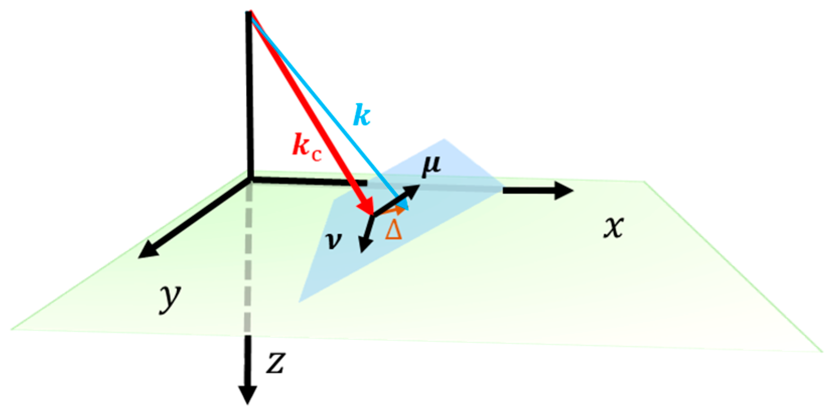
Figure 1 illustrates a schematic for a beam that has undergone a Fourier transform. In this study, under the condition that the incident beam is well-collimated, its angular spectra can be approximated as a narrow expansion around a central wavevector represents the wavelength), which is depicted by a black ray. The non-central wavevectors () can be expressed as the vector addition of the beam’s central wavevector and a small orthogonal deflection () [26]. Here, and are a set of orthogonal unit vectors along the direction of in-plane and out-of-plane incidence, respectively. Consequently, we have the following:
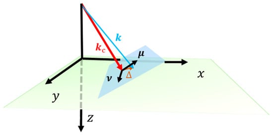
Figure 1.
A schematic for a paraxial approximation beam performed a Fourier transform; is its central wavevector (represented by a red ray); the non-central wave vector can be expressed as the vector addition of the beam’s central wavevector and a small orthogonal deflection (depicted by a brown ray). and are a set of orthogonal unit vectors along the direction of in and out of the plane of incidence, respectively.
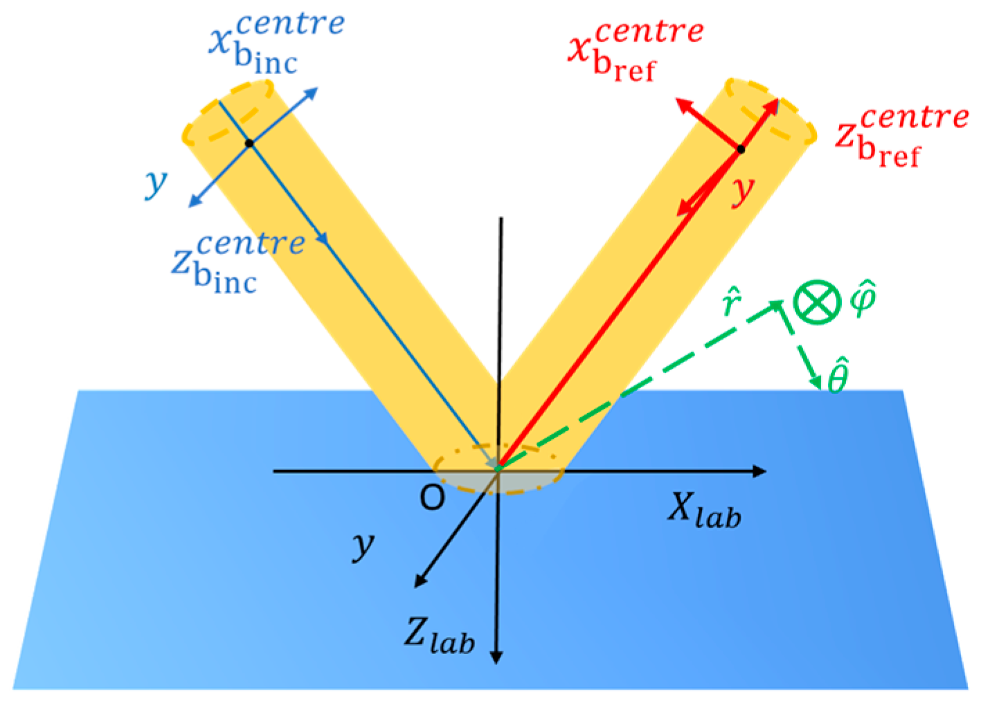
2.2. Frames of Reference and Coordinates in the Reflection Process of Light Beams
In the reflection process, two frames of reference are involved: the frame of the beam and the frame of the lab. These are represented by yellow beam-like shapes and blue rectangle, respectively, as shown in Figure 2. Four types of coordinates are established on each frame. The incident beam coordinates are depicted by three blue rays labelled ‘, , and ’; the reflected beam coordinates are shown by three red rays labelled; ‘, , and ’ the Cartesian lab coordinates are represented by three black rays labelled ‘, , ’; and the spherical lab coordinates are depicted by three green rays labelled ‘, , ’.
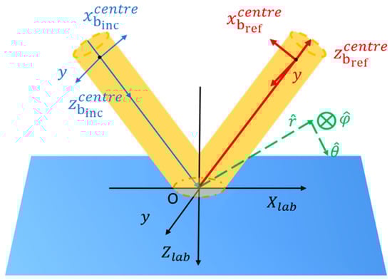
Figure 2.
Shows a schematic of two frames of reference (frames of lab and beam) and four coordinates system (incident and reflected beam coordinates; Cartesian lab coordinates and spherical lab coordinates) involved in the reflection process.
The two beam coordinates are mirror images of each other. The origin of the Cartesian lab coordinates is set at the incident point on the interface, which is defined as the intersection point between the central wave vector of the incident beam and the reflection interface. The central wave vector of the incident beam and the normal to the reflection interface lie within the plane. The direction perpendicular to this plane is defined as the -direction.
In addition, the spherical coordinate system within the laboratory frame is necessary for the study because of the following: 1. It allows for a convenient representation of the transform between non-central wave vectors and the central wave vector. 2. The electric field components and in the spherical coordinate correspond to the and polarisation states in the Fresnel equation. Consequently, building the laboratory spherical coordinate system will facilitate computations.
By rewriting the small orthogonal deflection () in the incident beam coordinates, we have the following:
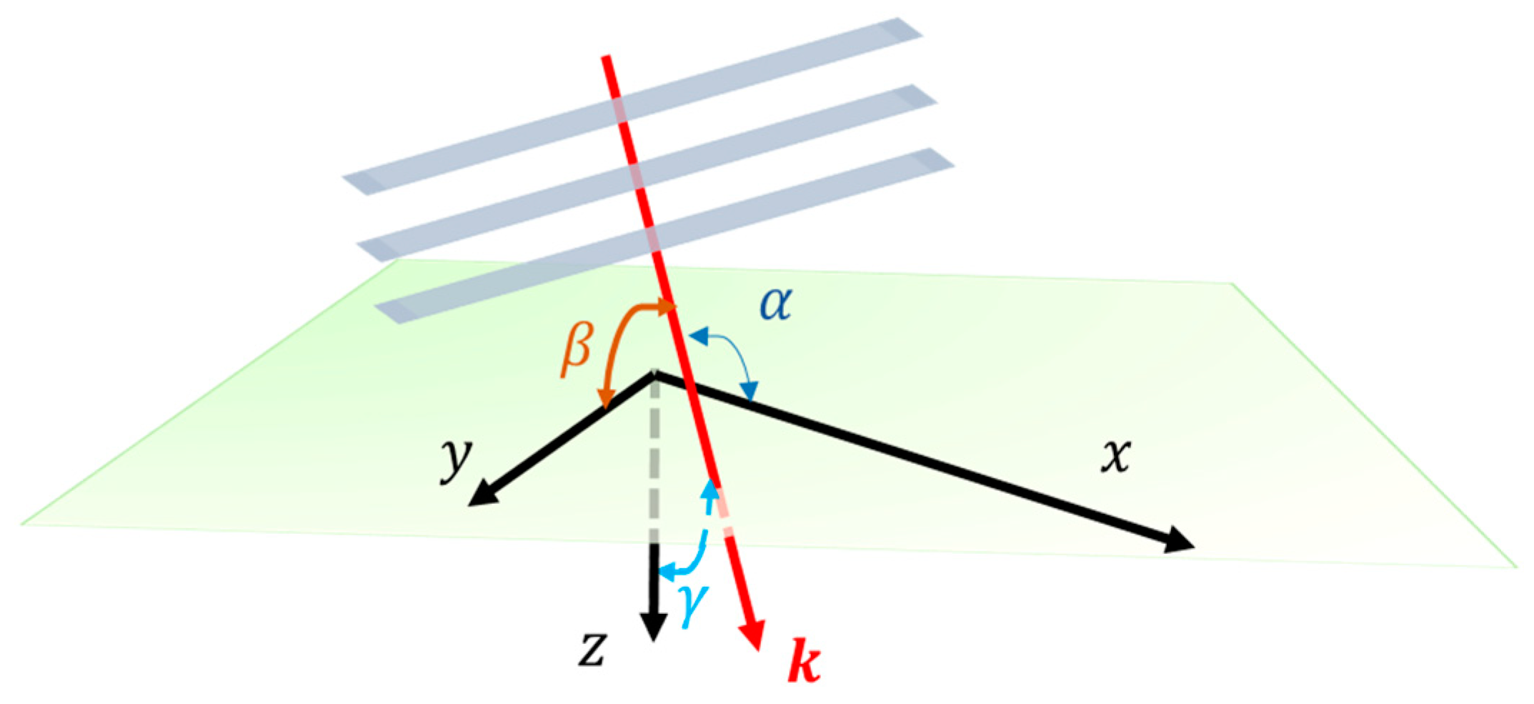
The angular spectrum method is commonly employed to obtain the spatial spectra of the incident beam [31]. To better understand the role the angular spectrum method played in this study, it is essential to review the concepts of plane waves and the angular spectrum method. Figure 3 is a schematic diagram of plane waves propagating in the free space:
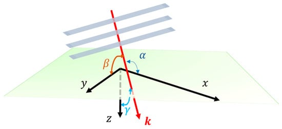
Figure 3.
The plane wave (represented by three grey planes) propagating along the direction of its wavevector (represented by a bright red ray). , , and are the angles between the plane wavevector and the axes, respectively.
The complex field expression of the plane wave in Cartesian coordinates is the following:
is the wavenumber, and , , are the angles between the plane wave vector and axes, respectively. The relationship between the three angles is the following:
This relation indicates that there are only two independent variables. Consequently, Equation (4) can be rewritten as follows:
In Fourier optics, Equation (5) is frequently rewritten as follows ( is wavelength) [32]:
Hence, ; .
Consequently, in the beam coordinate system, the non-central wave vectors, or the orthogonal deflection (), as demonstrated in Equation (3), can be reformulated as follows:
Moreover, we can find the following:
2.3. Calculation of Reflected Optical Fields on Dielectric Materials
It is natural to study the spatial spectra of the incident beam in the incident beam coordinates. However, using the frame of the lab with spherical coordinates is more convenient for calculating the ratios of reflected light to incident light using the Fresnel equation. Equation (12) illustrates the transformation of the incident light beam’s spectra from the beam coordinates to the lab spherical coordinates.
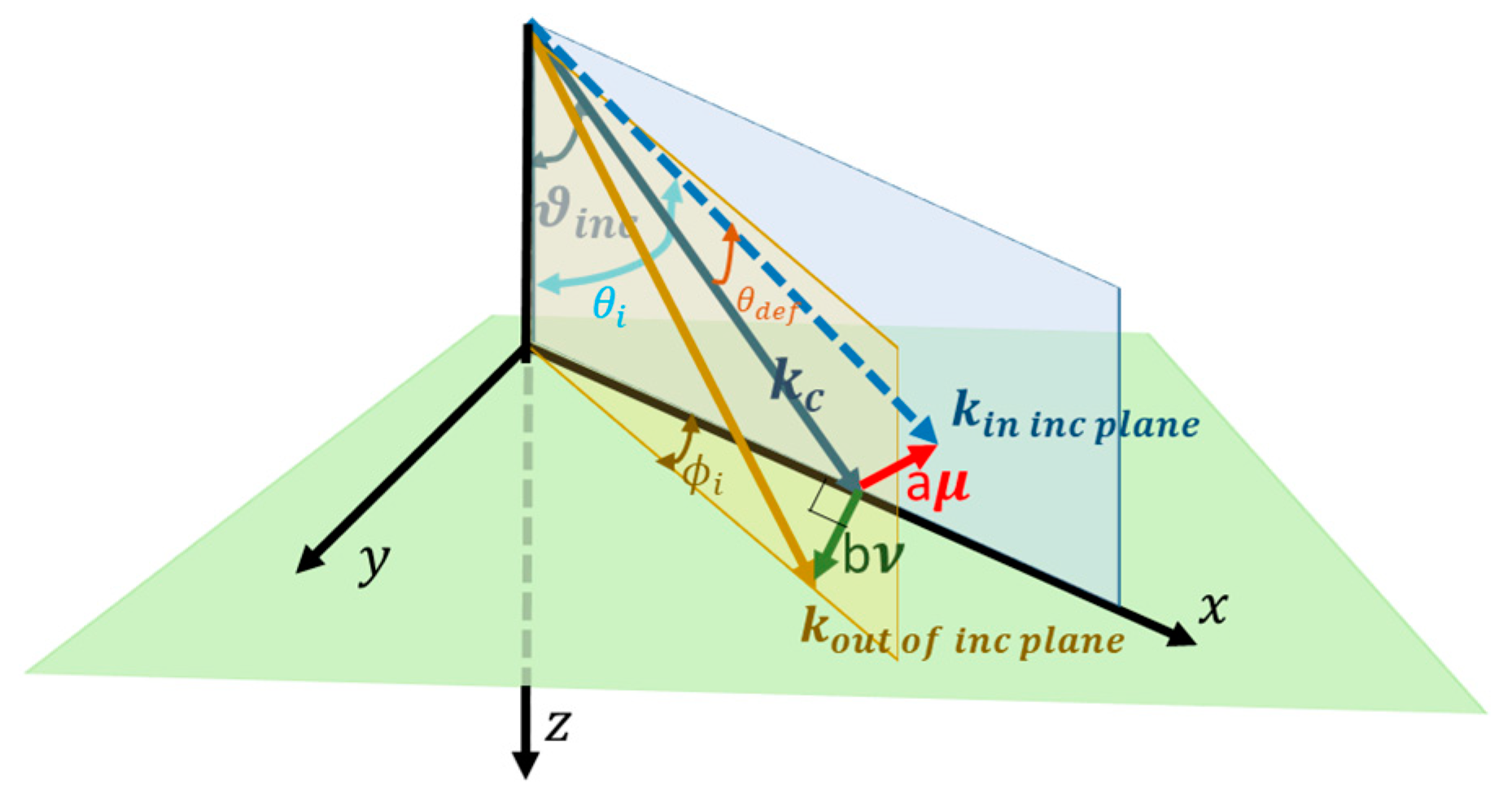
The symbol represents the magnitude of the angle between the central wave vector and the normal of the reflection surface. To determine the angles of incidence for non-central wave vectors, the relationships between non-central and central wave vectors must first be clarified. These relations involve the angles and . Equations (13) and (14) provide the expressions for these angles [30], and Figure 4 is the schematic illustrating them.
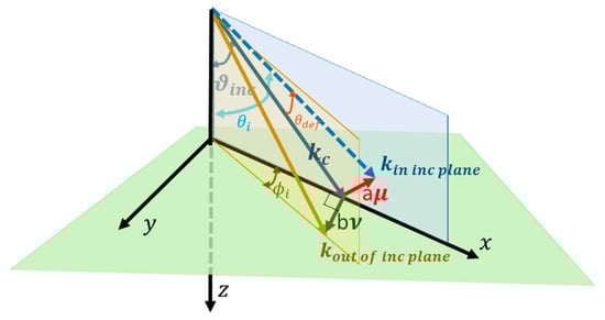
Figure 4.
The schematic for and . The (light blue dashed ray) represents the non-central wave vector within the incident plane defined by central wavevector (dark blue ray); The (brown ray) represents the non-central wave vector lies outside of the incident plane; The (red ray) and (dark green ray) are a set of orthogonal deflections along the direction of in and out of plane of incidence, respectively. The symbol represents the magnitude of the angle of central wave incidence. Moreover, is the angle between and .
When the transfer matrix [28,30] (, as shown in Equation (15)) is clear, the ratios of reflected light to the incident light can be calculated. The spectra of the reflected beam () are the following:
is the Fresnel Jones matrix [30], as shown in Equation (16). The symbols and represent the Fresnel coefficients associated with the polarisation components parallel () and orthogonal () to the plane of incidence, respectively. Using Taylor series expansion for spectral components around the central wave vector () and focusing solely on the initial expansion term, we can formulate the Fresnel Jones matrix [28,30]:
Therefore, the transfer matrix can be further elaborated as follows:
where represents the relative dielectric constant of the reflecting surface and expressions of and are the following:
3. Results
A computational model for VBs and VVBs reflection is developed using MATLAB. The parameters for the setup of the simulation are as follows: wavelength: 532 nm; beam width of the fundamental mode (the distance from the centre to points where the maximum intensity is found [33]): 13 µm; frame of the figure: 30 µm × 30 µm (drawing dimensions of optical fields); pixel array: 1024 × 1024 (The optical field distribution image features 1024 pixels in each of the horizontal and vertical directions).
3.1. Intensity and Polarisation Distribution of the Incident Beam and of the Reflected Beam at the Brewster Angle
VBs and, in particular, VVBs are natural solutions to the full vector wave equation [34], and more commonly, they are represented as the superposition of orthogonal scalar fields, which have orthogonal polarisation states [35], as shown in Equation (20):
We use the notation to represent a vector beam. The symbols and represent a pair of orthogonal eigenstates. Specifically, these eigenstates are right-circularly and left-circularly polarised LG beams, with OAM quantified as and , respectively. The symbols and represent the coefficients of these two eigenstates, which are defined by relative intensity (variables ) and relative phase ( []). In cof VB and VVB, which are the research objects in this work, will be introduced.
In this work, to avoid ambiguity, light beams with spatially variant or inhomogeneous polarisation but no phase vortices are referred to as VBs. Beams with both inhomogeneous polarisation and phase vortices are called VVBs. VBs carry no OAM, whereas VVBs carry OAM owing to their spiral phase fronts [36].
There are six different types of incident beams studied: radially polarised beams, three kinds of VBs with hybrid polarisation states, and ‘lemon’-polarised and ‘star’-polarised vortex beams. These incident beams can be expressed by the superposition of two eigenstates [37,38,39]:
- Radially polarised beams ();
- Vector beam with hybrid polarisation states ();
- Vector beam with hybrid polarisation states ();
- Vector beam with hybrid polarisation states ();
- ‘Lemon’-polarised vortex beams (, );
- ‘Star’-polarised vortex beams (, ).
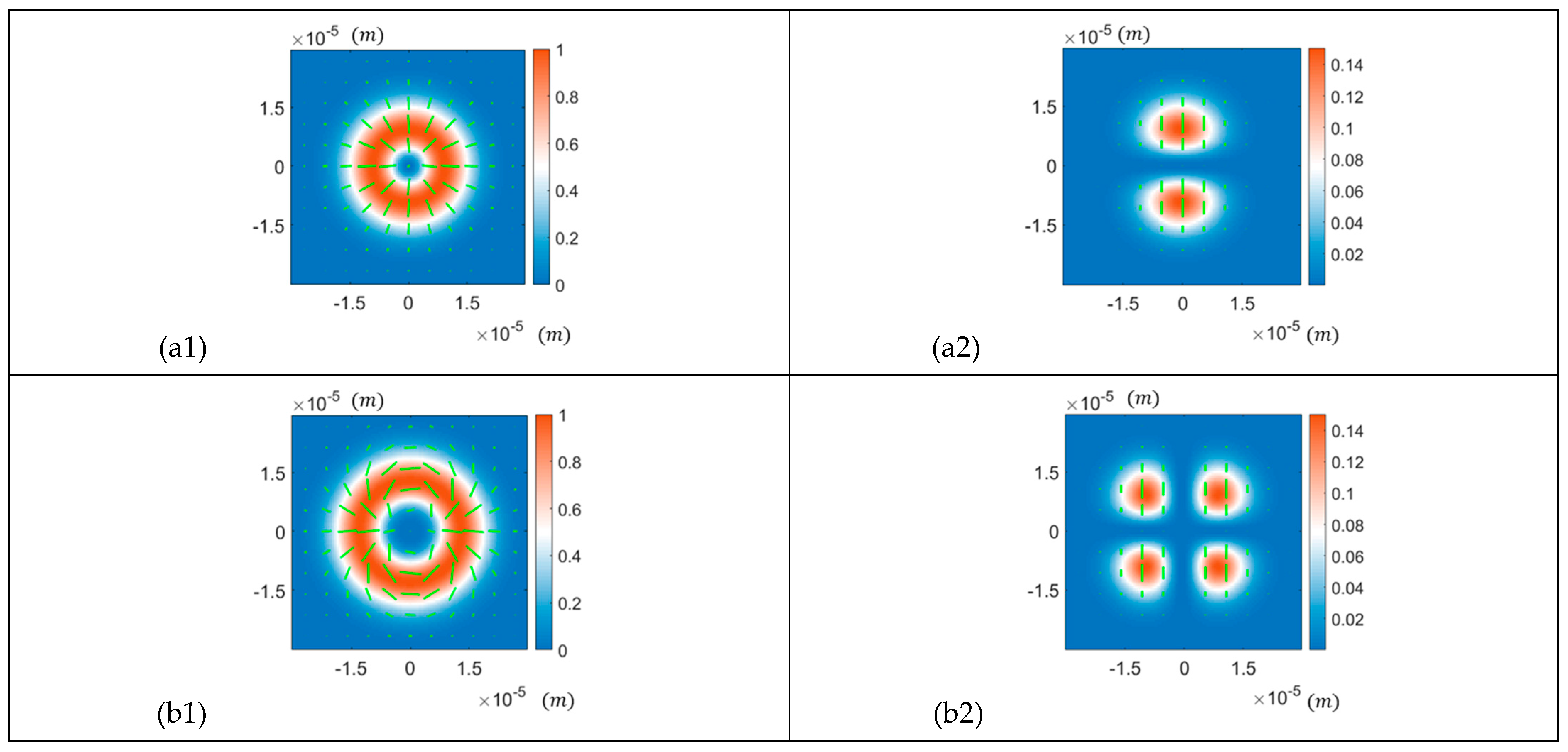
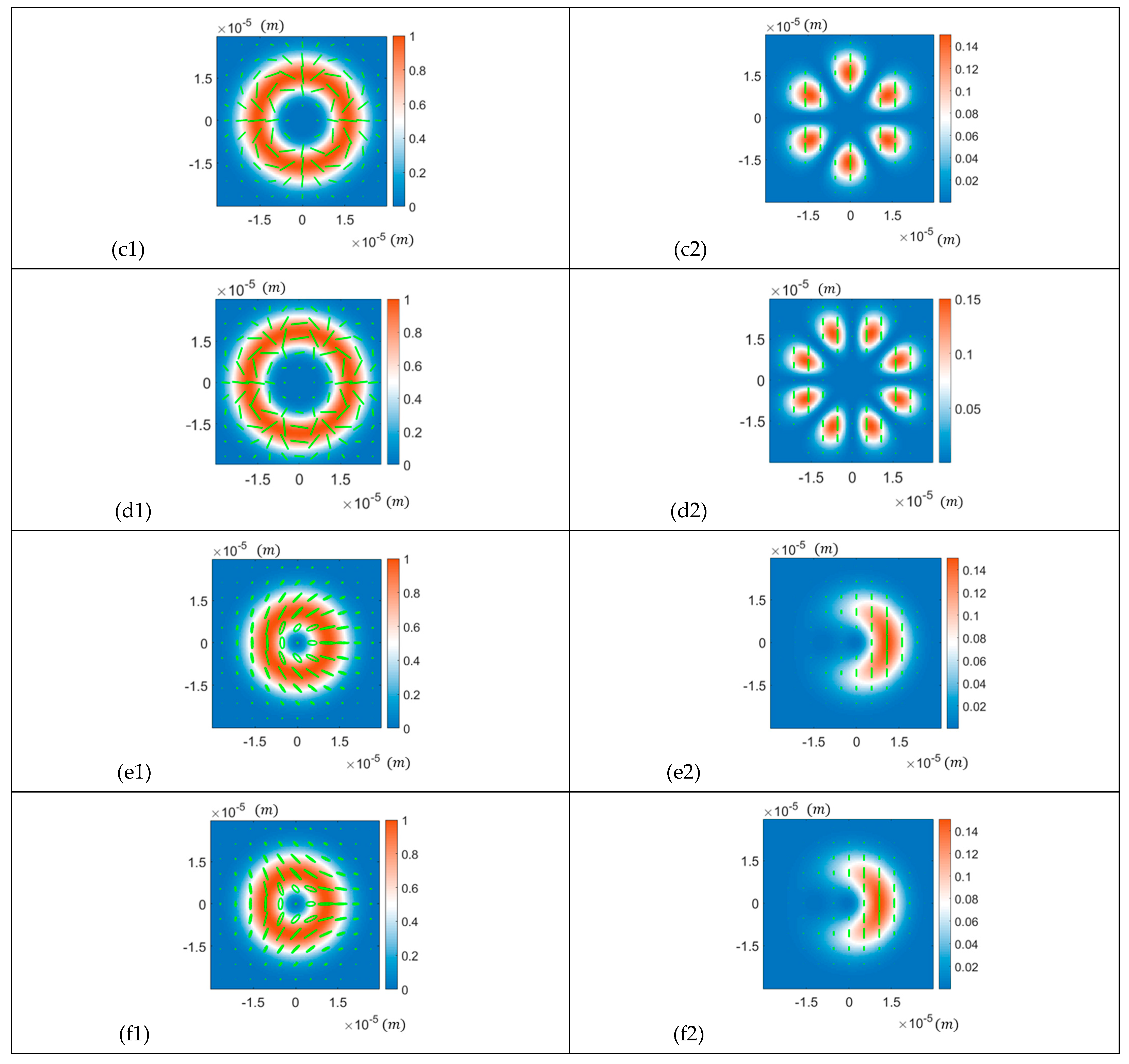
The Brewster angle is an important property for dielectric materials. In this study, the reflection surface is set as the glass, and its Brewster angle is around 56.6° [40]. When the angle of the incidence is equal to the material’s Brewster angle, only the S-wave component is reflected [41]. The polarisation state of the S-wave is orthogonal to the plane of incidence. Figure 5 shows the intensity and polarisation distribution of the six types of beams mentioned earlier. Because the OAM modes carried by eigenstates of these beams are not zero, their intensity distributions exhibit doughnut shapes, with vanishing intensity at the centre. The size of the lines, which represent the polarisation states of that area, is proportional to the intensity of that area. Consequently, the polarisation states at the centre of the images are depicted by small points. The colormap from blue to white to red indicates increasing intensity. There are two columns in the figure: the first column shows the intensity and polarisation distributions of six kinds of incident beams, and the second column displays those of their reflected beams when the incident angle is at the Brewster angle (56.6°).
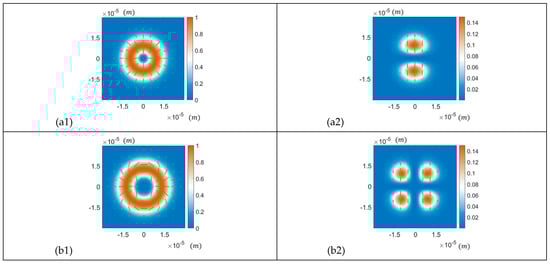
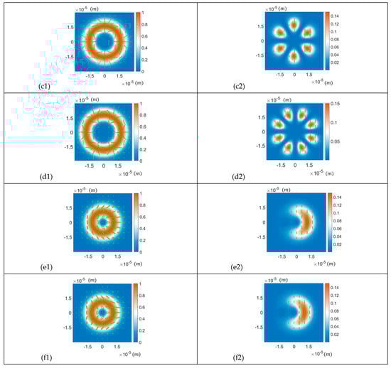
Figure 5.
The first column shows the intensity and polarisation distribution of the incident beams. From (a1) to (f1) are the radially polarised beam, three types of VBs with hybrid states of polarisation (, and , respectively), the ‘lemon’-polarised vortex beam, and the ‘star’-polarised vortex beam, respectively. The second column (from (a2) to (f2)) displays the intensity and polarisation distribution of the beams reflected on a glass surface when the incident angle is the Brewster angle (e.g., (a2) is the reflected beam of (a1)). Since the OAM modes carried by the above beams are not zero, their intensity distributions have doughnut shapes, with vanishing intensity at the centre. The size of the lines (representing polarisation states of that area) in the images is proportional to the intensity of that area; consequently, the polarisation states at the centre of the images are small points. The colormap from blue to white to red indicates increasing intensity.
3.2. Intensity Distribution of the Incident Beam and the Optical Field Reflected at the Brewster Angle in Azimuthal and Radial Coordinates ()
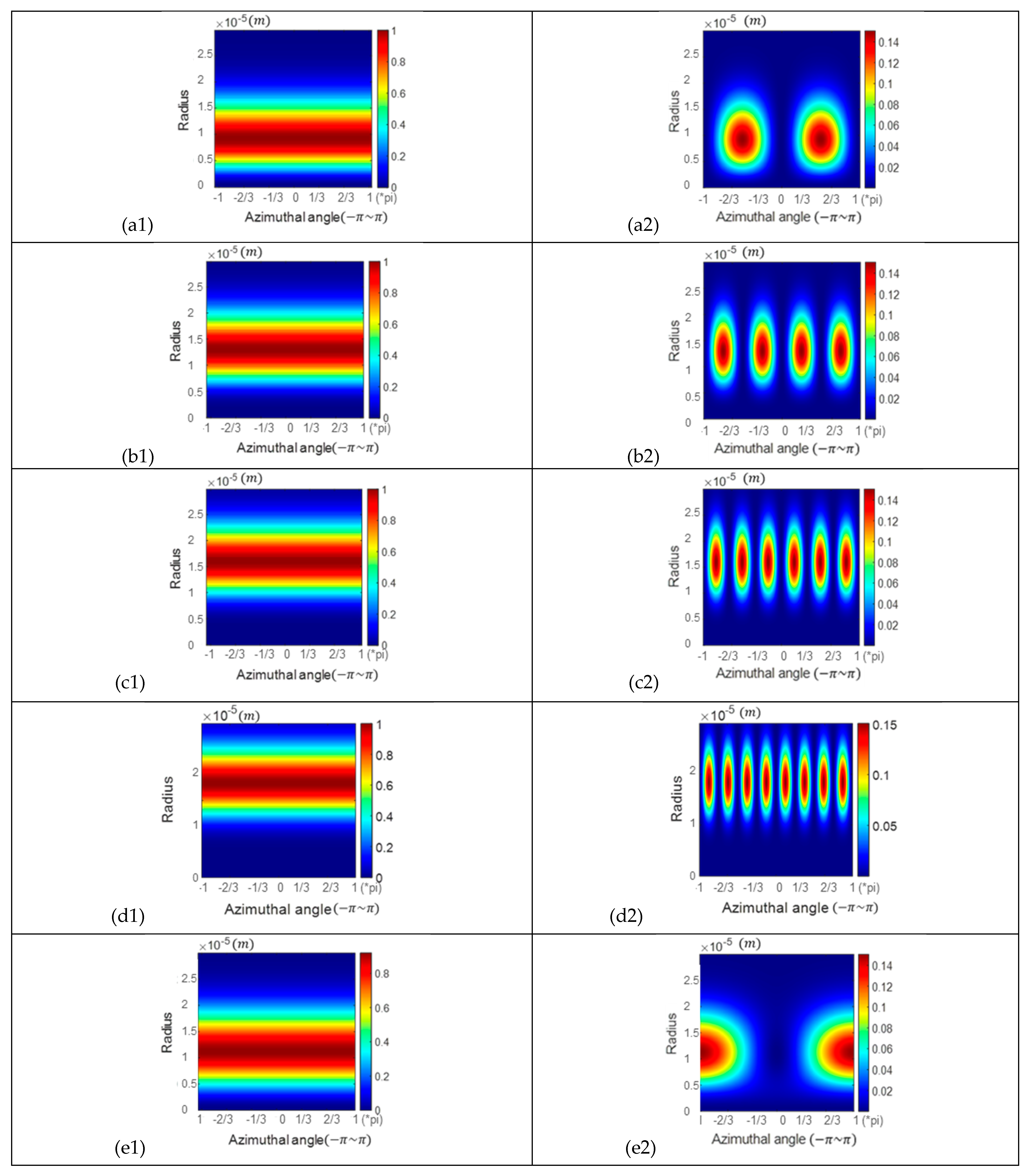
The reflected field, plotted in azimuthal and radial coordinates (), is studied. This approach provides us with another perspective to analyse the reflected field from different incident angles. The first column in Figure 6 displays the intensity distribution of the six kinds of incident beams plotted in a new coordinate system: azimuth () and radial coordinates (0~30 µm). The intensity is normalised. It can be observed that the intensity distributions of these six incident beams exhibit symmetry along the azimuthal direction. The intensity distributions of these beams at the Brewster angle are also examined, and results are shown in the second column of Figure 6. The colormap from dark blue to dark red indicates increasing intensity.
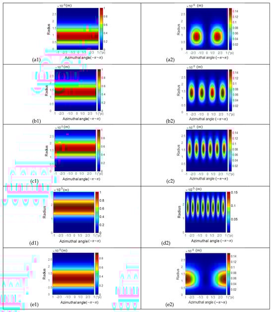
Figure 6.
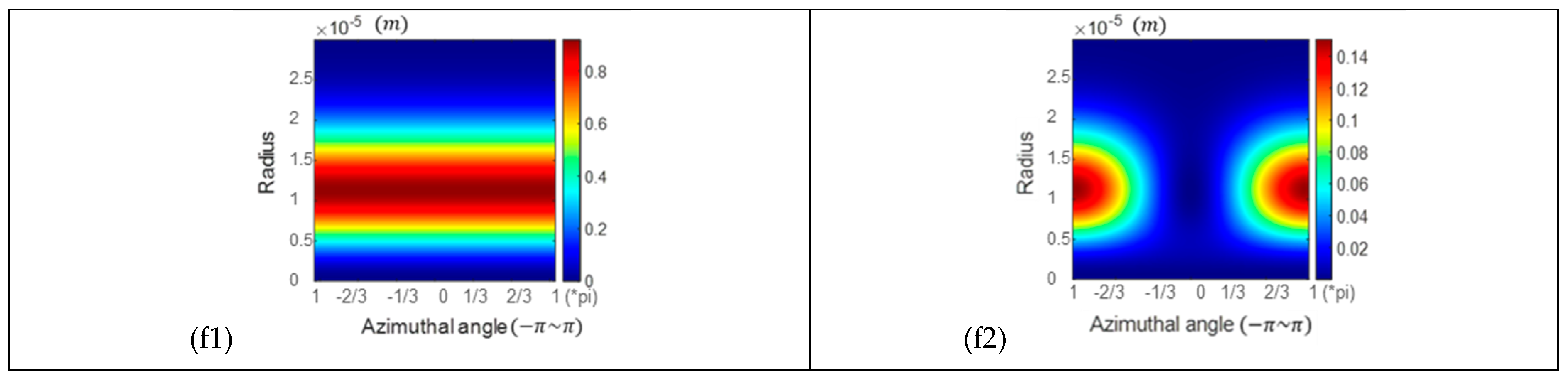
The first column shows the intensity distribution of the incident beams. From (a1) to (f1) are the radially polarised beam, three types of VBs with hybrid states of polarisation (, and , respectively), the ‘lemon’-polarised vortex beam, and the ‘star’-polarised vortex beam, respectively. The second column (from (a2) to (f2)) displays the intensity distribution of the beams reflected on a glass surface when the incident angle is the Brewster angle (e.g., (a2) is the reflected beam of (a1)). These intensity distributions of incident beams arranged in the first column and reflected beams arranged in the second column are plotted in a new coordinate system: azimuth () and radial coordinates (0~30 µm). The colormap from dark blue to dark red indicates increasing intensity.
According to the intensity distributions shown in Figure 6, we observe that these beams have different beam widths. For the beams’ eigenstates carrying OAM, the beam width is generally positively proportional to the modulus of the OAM. The eigenmodes’ OAM of the four types of VBs (radially polarised beam and three types of VBs with hybrid states of polarisation) are , and , respectively. Regarding the ‘lemon’- and ‘star’-polarised vortex beams, their eigenmodes include OAM modes with moduli 1 and 2, respectively. Therefore, the beam widths of the six types of incident beams are arranged in ascending order: radially polarised beam ‘lemon’ ‘star’ VB with hybrid states of polarisation ( VB with hybrid states of polarisation ( VB with hybrid states of polarisation (.
4. Discussion
In this section, properties of the reflection field are explored and analysed: First, the variation of reflectivity with the incident angle is investigated. Next, the displacement of the intensity centroid of the reflected beam relative to the frame’s centre is examined. Finally, the range of intensity of the reflected beam in () coordinates is analysed.
4.1. Reflectance Variation across Incident Angles from 1° to 85°
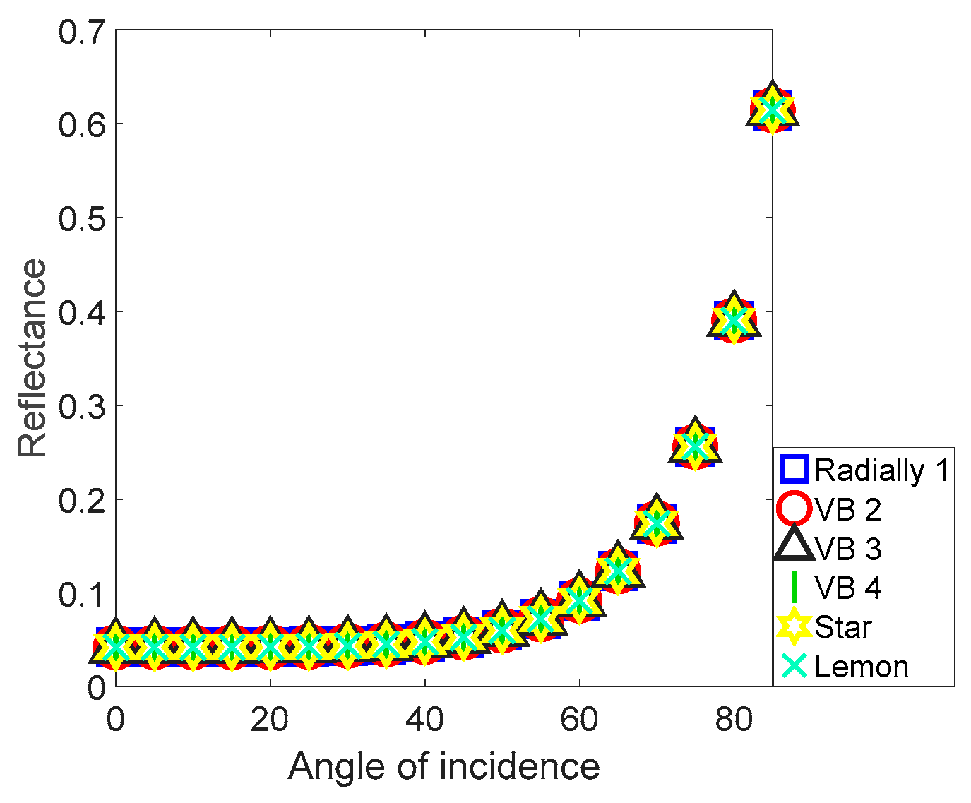
The reflectance of six types of beams reflected at a glass surface is investigated, and the result is shown in Figure 7. The incident angle range is (1°~85°), with the reflectance trends of different incident beams plotted using various colours and markers as indicated in the legend.

Figure 7.
Trends of reflectance versus the incident angle. There are six kinds of beams studied: the radially polarised beam, three types of VBs with hybrid states of polarisation (denoted as ‘VB2′ to ‘VB4′ corresponding to , , and , respectively.), the ‘lemon’-polarised vortex beam, and the ‘star’-polarised vortex beams. These beams are reflected at the glass surface over an incident angle range of 1° to 85°.
In Figure 7, it can be observed that all curves overlap. More precisely, their trends are identical. This suggests that reflectance is independent of the type of incident beam but depends on the interface material and incident angle, as predicted by the Fresnel equations Equations (18) and (19). Using VBs and VVBs as the light source for LiDAR, the orientation of the reflective surface can be deduced by measuring the reflectance.
4.2. Shift in the Intensity Centroid of Reflected Beams across Incident Angles from 1° to 89°
Due to the Fresnel equations, different polarisation components of light exhibit varying reflectance, resulting in a noticeable variation in the intensity distribution of the reflected field with changes in the incident angle, which indicates that we can find the relationship between the centroid of the intensity distribution of the reflected light field and the incident angle.
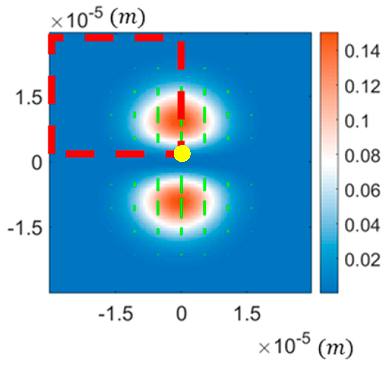
Firstly, we investigated the intensity distribution of four types of VBs and found that their reflected light field exhibits central symmetry. Figure 8 illustrates the reflected field of the radially polarised beam as an example. The central symmetry of a radially polarised beam implies that the centroid of its intensity distribution remains at the centre of the image, independent of the incident angle. Consequently, one cannot directly deduce the relationship between the centroid of the reflected beam’s intensity distribution and the incident angle. To address this issue, we extracted a quarter of the reflection field’s intensity distribution and determined the centroid of this quarter part. Specifically, the reflection field image comprises 1024 × 1024 pixels, but we analysed only the upper left 512 × 512 pixels. This is illustrated in Figure 8.
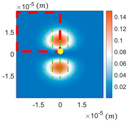
Figure 8.
The extracted quarter part (the section framed by red dotted lines) of a reflected field, which is used to analyse the shift of the intensity centroid. The yellow point represents the centre of the original image.
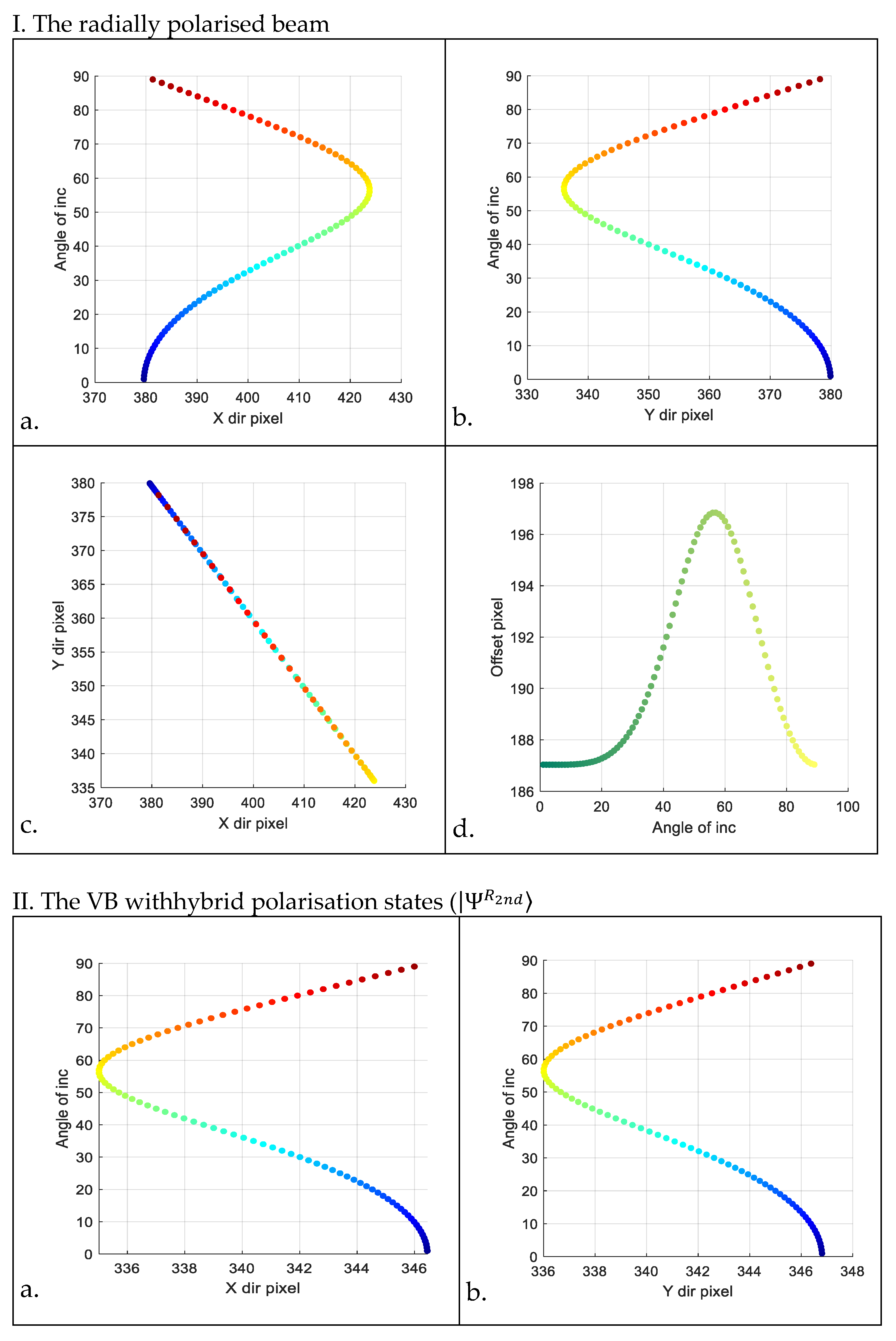
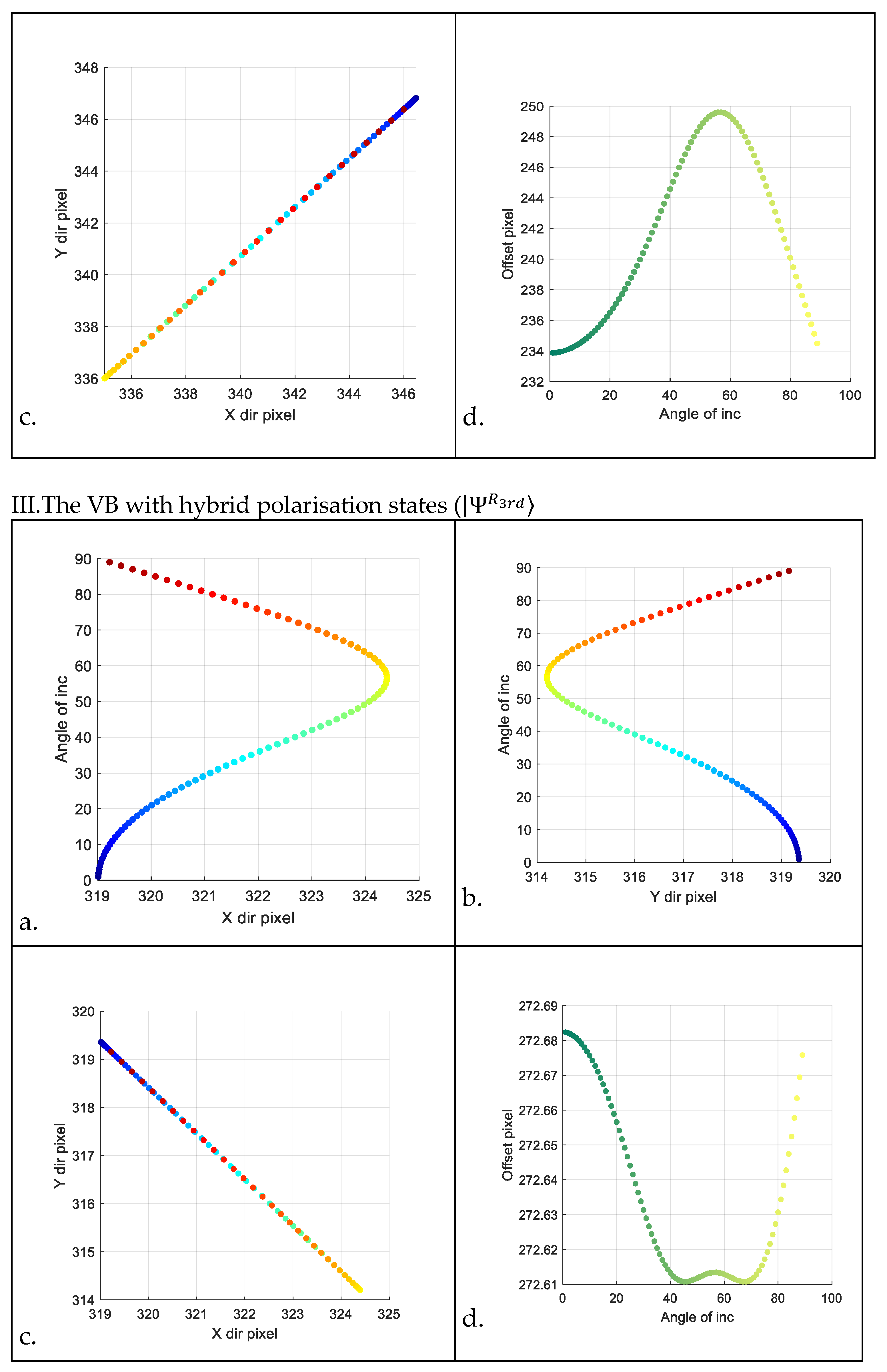
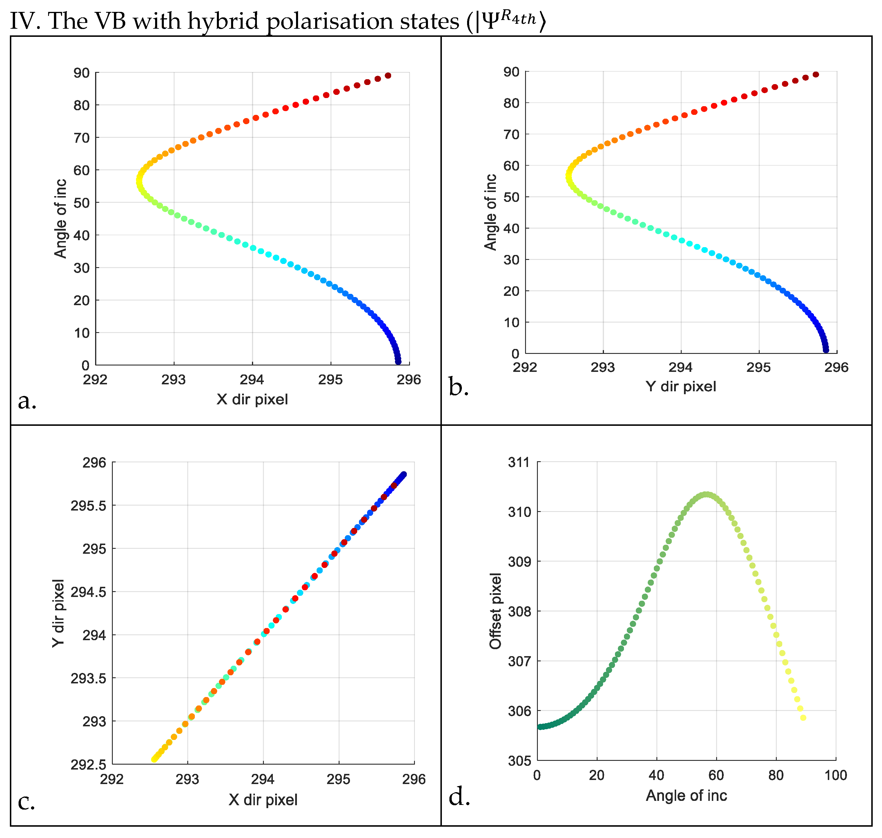
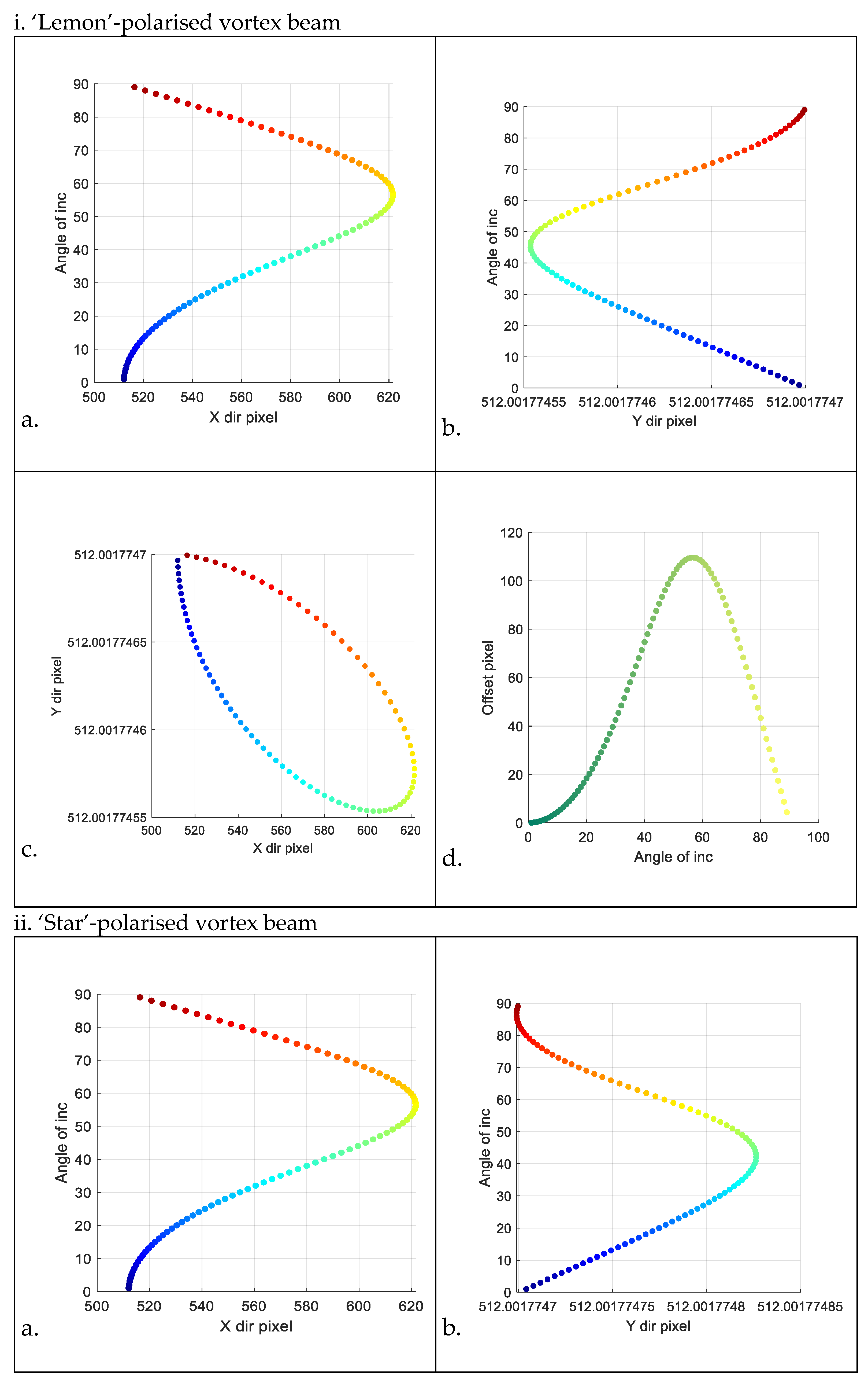
The relationship between the centroid shift in the reflected light field and the incident angle is demonstrated in four graphs. For example, in group (I) of Figure 9, the following four graphs are presented: 1. the relationship between pixel position in the x-direction of the centroid and the incident angle; 2. the relationship between pixel position in the y-direction of the centroid and the incident angle; 3. the centroid’s movement across the transverse field of the reflected beam varying with the incident angle (colours ranging from blue to reddish brown indicate increasing incident angles); 4. the variation in Euclidean distance from the centroid to the original image centre (referred to as centroid offset distance) with respect to the incident angle (colours ranging from dark green to shallow yellow indicate increasing incident angles).
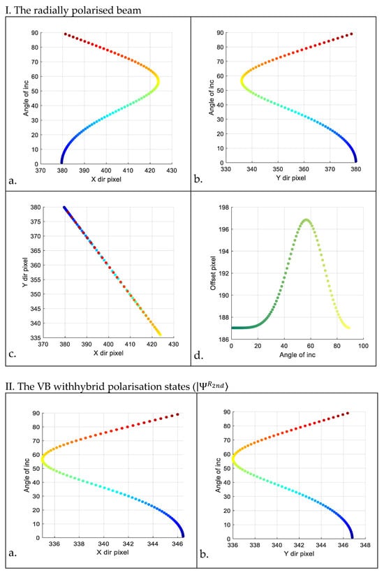
Figure 9.
Four groups of graphs. Groups labelled ‘(I)’ through ‘(IV)’ represent the radially polarised beam and three types of VBs with hybrid polarisation states, respectively. Each group includes four images labelled (a) through (d): (a). the relation between pixel position in the x-direction of the centroid and the incident angle; (b). the relation between pixel position in the y-direction of the centroid and the incident angle; (c). the centroid’s motion within the transverse field of the reflected beam varying with the incident angle (colours ranging from blue to reddish brown indicate increasing incident angles (1°~89°)); (d). the variation in Euclidean distance (referred to as ‘offset pixel’ in the diagram) from the centroid to the original image centre (depicted as a yellow point in Figure 8) with respect to the incident angle (colours ranging from dark green to shallow yellow indicate increasing incident angles (1°~89°)).
We observe that each incident angle corresponds to a specific coordinate of the centroid. However, near the Brewster angle, the Euclidean distance from the centroid to the image centre exhibits nearly axisymmetric characteristics. Additionally, the centroid coordinates of the intensity distribution of the reflected light field shift in the opposite direction at the Brewster angle, and the centroids of some large-angle incident reflection fields approximately overlap with those of small-angle incident fields.
By comparing panels (a) and (b) of the four types of VBs in Figure 9, we find that the coordinate shifts of the intensity centroid of the radially polarised beam are larger. Furthermore, we can determine the order of the coordinate shifts of the intensity centroid of the reflected field in the x and y directions, from largest to smallest, as the incident angle varies: radially polarised beam > VB with hybrid polarisation states ( > VB with hybrid states of polarisation (> VB with hybrid states of polarisation (. Additionally, according to panels (d) of the four types of VBs, the distribution of offset pixels is axisymmetric with respect to the Brewster angle axis. This suggests that deducing the incident angle solely from the centroid coordinates or the centroid’s offset distance relative to the centre of the image is a challenge. To ascertain whether the incident angle is less than or greater than the Brewster angle, it is necessary to measure the energy of the reflected field.
Additionally, the change in the shift of the intensity centroid of the reflected field for ‘lemon’- and ‘star’-polarised vortex beams is also characterised. Unlike the four VBs, the intensity distribution of the reflected fields of these two no longer exhibits rotational symmetry relative to the centre of the image. Consequently, in the following section, there is no partial extraction analysis of the intensity distribution of the reflected field. All results are shown in Figure 10.
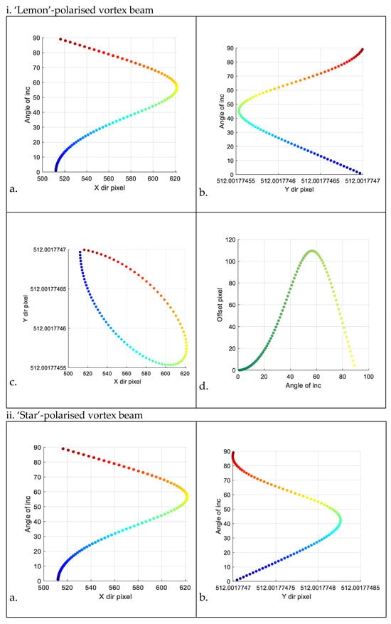
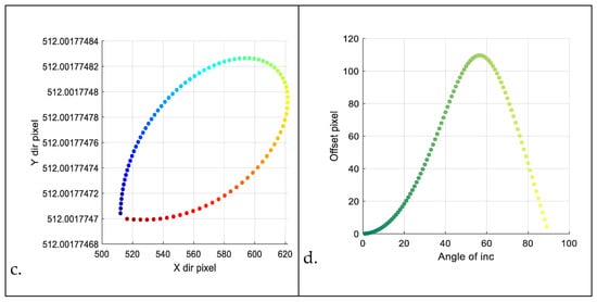
Figure 10.
Two groups of images. Groups labelled (i) and (ii) represent ‘lemon’- and ‘star’-polarised beams, respectively. Each group includes four images labelled (a) through (d): (a) the relation between pixel position in the x-direction of the centroid and the incident angle; (b). the relation between pixel position in the y-direction of the centroid and the incident angle; (c). the centroid’s motion within the transverse field of the reflected beam varying with the incident angle (colours ranging from blue to reddish brown indicate increasing incident angles (1°~89°)); (d). the variation in Euclidean distance (referred to as ‘offset pixel’ in the diagram) from the centroid to the image centre (depicted as a yellow point in Figure 8) with respect to the incident angle (colours ranging from dark green to shallow yellow indicate increasing incident angles (1°~89°)).
It can be observed that the shift in the intensity centroid of the two types of VVBs is almost the same: the centroid moves primarily in the x-direction, and according to the panels (b) of the two VVBs, we can see that the centroid remains nearly unchanged in the -direction. Additionally, the range of the centroid shift in the -direction is much larger than that of the four types of VBs. The axial symmetry shown in two panels (d) is similar to that of the four types of VBs; the distribution of offset pixels is axisymmetric with respect to the Brewster angle axis. However, unlike those four VBs, the range of the pixel coordinate shifts of the intensity centroid of the reflected field relative to the pixel coordinates of the field origin is larger. Deducing the value of the incident angle from the pixel coding coordinates of the centroid of the reflected field intensity may not be sufficient. However, in scenarios where the incident angle is smaller than the Brewster angle, or the target object undergoes small-axis rotation, the incident angle can be deduced solely from the coordinates of the centroid of the reflected field intensity. Moreover, when focusing solely on the range of the pixel coordinate shifts of the intensity centroid of the reflected field relative to the pixel coordinates of the field origin, using ‘lemon’ and ‘star’-polarised vortex beams as detection signals is better.
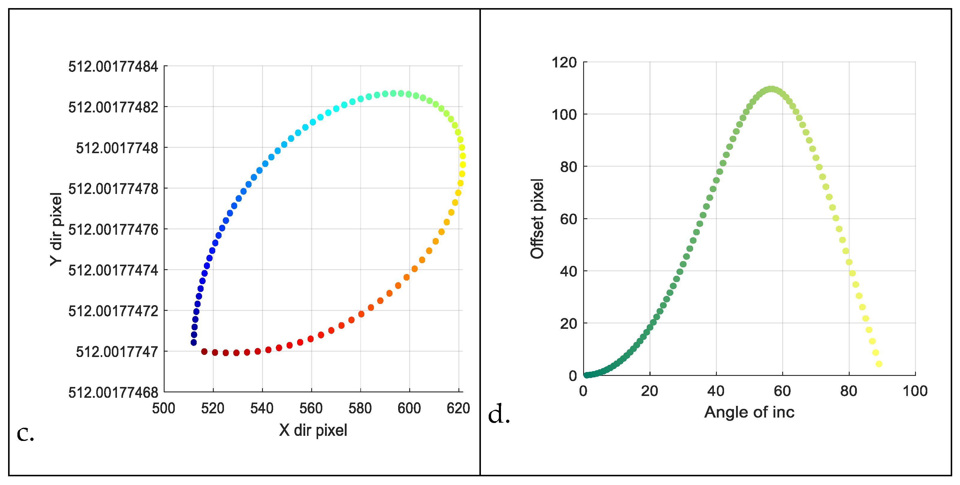
4.3. Range of the Intensity of the Reflected Fields in the () Coordinates
Although the intensity distributions of the six types of incident beams are rotational symmetric (as shown in Figure 6), their intensity remains unchanged along the direction, and the intensity distributions of the reflected beams no longer remain unchanged along the direction. This inspired this study to find the relationship between the angle of incidence and intensity distribution of the reflected beam.
Therefore, we extracted the reflected beams’ intensity data for all points at coordinates r = 11.28 µm. Then the minimum value and maximum value are found to calculate range of the intensity. We examined the intensity ranges of the reflected beams for incident angles ranging from 1° to 89°. Figure 11 shows graphs of the relation of the angle of incidence and the intensity range.
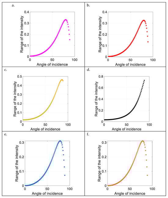
Figure 11.
The relationship between the angle of incidence and the intensity range. The intensity data of the reflected beams (in the () coordinates) at all points with r = 11.28 µm are extracted, and the minimum value and maximum value are determined to calculate the range. The intensity ranges of the reflected beams for incident angles ranging from 1° to 89° are examined. Panels (a–f) correspond to the radially polarised beam, three types of VBs with hybrid states of polarisation (, and , respectively), ‘lemon’-polarised vortex beam, and ‘star’-polarised vortex beams, respectively.
Based on the above graphs, several characteristics can be observed:
- Except for the VB with hybrid states of polarisation , the trend of the other five types of beams shows multivalued properties;
- Range of the intensity of the VB with hybrid states of polarisation is greater than that of other beams;
- For the four types of VBs, the higher the modulus of OAM carried by their eigenstates, the better the performance in deducing the incident angle from the intensity range;
- The trends shown in graphs (e) and (f) of the lemon’-polarised and ‘star’-polarised vortex beams are the same.
In experiments and practical engineering, we can use area-array CCDs and line-array CCDs to measure the intensity distribution of the light field. Line-array CCDs are more widely used in practical applications. This is because area-array CCDs are expensive, while line-array CCDs are more affordable and can be manufactured with many pixels. By using a line-array CCD in conjunction with a scanning mechanism and position feedback system, the radial intensity distribution of the light field mentioned in the text can be measured. Then, the measurement of the orientation of the reflecting surface can be achieved.
5. Conclusions
In this paper, the potential of using VBs and VVBs as detection signals for LiDAR sensors to measure the orientation of reflecting surfaces is explored. We develop a computational model for these beams’ reflection. With the help of this model, the relationship between the properties of reflected optical fields and incident angles, focusing on reflectance, intensity centroid shifts, and the intensity range of the reflected beam in the azimuthal direction, is examined. The findings suggest that the ‘lemon’- and ‘star’-polarised vortex beams are good choices among the six types of beams, as their ranges of the centroid shift in the x direction are much larger. Additionally, the vector beam with hybrid states of polarisation ( stands as another good choice because its range of intensity variation correlates monotonically with the incident angle, and this range is greater than that of the other five types of beams. In summary, this work provides a new sensing scheme for LiDAR research.
Author Contributions
Conceptualisation, W.Y. and J.Y.; methodology, W.Y.; software, W.Y.; validation, W.Y. and J.Y.; formal analysis, W.Y.; investigation, W.Y.; resources, J.Y.; data curation, W.Y.; writing—original draft preparation, W.Y.; writing—review and editing, J.Y.; supervision, J.Y.; All authors have read and agreed to the published version of the manuscript.
Funding
This research was funded by the Engineering and Physical Sciences Research Council EP/V000624/1.
Institutional Review Board Statement
The authors declare that they have NO affiliations with or involvement in any organisation or entity with any financial interest in the subject matter or materials discussed in this manuscript.
Informed Consent Statement
Not applicable.
Data Availability Statement
The data that support the findings of this study are available upon reasonable request from the authors.
Conflicts of Interest
The authors declare no conflicts of interest.
References
- Kolb, A.; Barth, E.; Koch, R.; Larsen, R. Time-of-flight cameras in computer graphics. Comput. Gr. Forum 2010, 29, 141–159. [Google Scholar] [CrossRef]
- Sarbolandi, H.; Plack, M.; Kolb, A. Pulse Based Time-of-Flight Range Sensing. Sensors 2018, 18, 1679. [Google Scholar] [CrossRef]
- Lange, R.; Seitz, P. Solid-state time-of-flight range camera. IEEE J. Quantum Electron. 2001, 37, 390–397. [Google Scholar] [CrossRef]
- Hansard, M.; Lee, S.; Choi, O.; Horaud, R.P. Time-of-Flight Cameras: Principles, Methods and Applications; Springer Science & Business Media: Berlin/Heidelberg, Germany, 2012. [Google Scholar]
- Uttam, D.; Culshaw, B. Precision time domain reflectometry in optical fiber systems using a frequency modulated continuous wave ranging technique. J. Light. Technol. 1985, 3, 971–977. [Google Scholar] [CrossRef]
- Wojtkiewicz, A.; Misiurewicz, J.; Nalecz, M.; Jedrzejewski, K.; Kulpa, K. Two-dimensional signal processing in FMCW radars. In Proceedings of the XXth National Conference on Circuit Theory and Electronic Networks; University of Mining and Metallurgy: Kolobrzeg, Poland, 1997; pp. 475–480. [Google Scholar]
- Elsayed, H.; Shaker, A. From Stationary to Mobile: Unleashing the Full Potential of Terrestrial LiDAR through Sensor Integration. Can. J. Remote Sens. 2023, 49, 2285778. [Google Scholar] [CrossRef]
- Guo, Q.; Su, Y.; Hu, T. LiDAR Principles, Processing and Applications in Forest Ecology; Elsevier Science: Amsterdam, The Netherlands, 2023. [Google Scholar]
- Wang, R. 3D building modeling using images and LiDAR: A review. Int. J. Image Data Fusion 2013, 4, 273–292. [Google Scholar] [CrossRef]
- Li, Y.; Zhao, L.; Chen, Y.; Zhang, N.; Fan, H.; Zhang, Z. 3D LiDAR and multi-technology collaboration for preservation of built heritage in China: A review. Int. J. Appl. Earth Obs. Geoinf. 2023, 116, 103156. [Google Scholar] [CrossRef]
- Li, Y.; Ibanez-Guzman, J. Lidar for autonomous driving: The principles, challenges, and trends for automotive lidar and perception systems. IEEE Signal Process. Mag. 2020, 37, 50–61. [Google Scholar] [CrossRef]
- Di Stefano, F.; Chiappini, S.; Gorreja, A.; Balestra, M.; Pierdicca, R. Mobile 3D scan LiDAR: A literature review. Geomat. Nat. Hazards Risk 2021, 12, 2387–2429. [Google Scholar] [CrossRef]
- Berezhnyy, I. A combined diffraction and geometrical optics approach for lidar overlap function computation. Opt. Lasers Eng. 2009, 47, 855–859. [Google Scholar] [CrossRef]
- Nape, I.; Singh, K.; Klug, A.; Buono, W.; Rosales-Guzman, C.; McWilliam, A.; Franke-Arnold, S.; Kritzinger, A.; Forbes, P.; Dudley, A.; et al. Revealing the invariance of vectorial structured light in complex media. Nat. Photonics 2022, 16, 538–546. [Google Scholar] [CrossRef]
- Yu, W.; Pi, H.; Taylor, M.; Yan, J. Geometric Representation of Vector Vortex Beams: The Total Angular Momentum-Conserving Poincaré Sphere and Its Braid Clusters. Photonics 2023, 10, 1276. [Google Scholar] [CrossRef]
- Cvijetic, N.; Milione, G.; Ip, E.; Wang, T. Detecting lateral motion using light’s orbital angular momentum. Sci. Rep. 2015, 5, 15422. [Google Scholar] [CrossRef]
- Fang, L.; Wan, Z.; Forbes, A.; Wang, J. Vectorial doppler metrology. Nat. Commun. 2021, 12, 4186. [Google Scholar] [CrossRef] [PubMed]
- Fu, S.; Guo, C.; Liu, G.; Li, Y.; Yin, H.; Li, Z.; Chen, Z. Spin-orbit optical Hall effect. Phys. Rev. Lett. 2019, 123, 243904. [Google Scholar] [CrossRef] [PubMed]
- Ahlawat, L.; Kishor, K.; Sinha, R.K. Photonic spin Hall effect-based ultra-sensitive refractive index sensor for haemoglobin sensing applications. Opt. Laser Technol. 2024, 170, 110183. [Google Scholar] [CrossRef]
- Bliokh, K.Y.; Nori, F. Relativistic hall effect. Phys. Rev. Lett. 2012, 108, 120403. [Google Scholar] [CrossRef] [PubMed]
- Jhajj, N.; Larkin, I.; Rosenthal, E.W.; Zahedpour, S.; Wahlstrand, J.K.; Milchberg, H.M. Spatiotemporal optical vortices. Phys. Rev. X 2016, 6, 031037. [Google Scholar] [CrossRef]
- Gui, G.; Brooks, N.J.; Kapteyn, H.C.; Murnane, M.M.; Liao, C.T. Second-harmonic generation and the conservation of spatiotemporal orbital angular momentum of light. Nat. Photonics 2021, 15, 608–613. [Google Scholar] [CrossRef]
- Gui, G.; Brooks, N.J.; Wang, B.; Kapteyn, H.C.; Murnane, M.M.; Liao, C.T. Single-frame characterization of ultrafast pulses with spatiotemporal orbital angular momentum. ACS Photonics 2022, 9, 2802–2808. [Google Scholar] [CrossRef] [PubMed]
- Mazanov, M.; Sugic, D.; Alonso, M.A.; Nori, F.; Bliokh, K.Y. Transverse shifts and time delays of spatiotemporal vortex pulses reflected and refracted at a planar interface. Nanophotonics 2022, 11, 737–744. [Google Scholar] [CrossRef]
- Hosten, O.; Kwiat, P. Observation of the spin Hall effect of light via weak measurements. Science 2008, 319, 787–790. [Google Scholar] [CrossRef] [PubMed]
- Bliokh, K.Y.; Bliokh, Y.P. Polarization, transverse shifts, and angular momentum conservation laws in partial reflection and refraction of an electromagnetic wave packet. Phys. Review. E Stat. Nonlinear Soft Matter Phys. 2006, 75, 066609. [Google Scholar] [CrossRef] [PubMed]
- Li, H.Y.; Wu, Z.S.; Shang, Q.C.; Bai, L.; Li, Z.J. Reflection and transmission of Laguerre Gaussian beam from uniaxial anisotropic multilayered media. Chin. Phys. B 2017, 26, 034204. [Google Scholar] [CrossRef]
- Zhen, W.; Wang, X.L.; Ding, J.; Wang, H.T. Controlling the symmetry of the photonic spin Hall effect by an optical vortex pair. Phys. Rev. A 2023, 108, 023514. [Google Scholar] [CrossRef]
- Ou, J.; Jiang, Y.; Zhang, J.; He, Y. Reflection of Laguerre–Gaussian beams carrying orbital angular momentum: A full Taylor expanded solution. J. Opt. Soc. Am. A 2013, 30, 2561–2571. [Google Scholar] [CrossRef]
- Andrews, D.L.; Babiker, M. (Eds.) The Angular Momentum of Light; Cambridge University Press: Cambridge, UK, 2012. [Google Scholar]
- Goodman, J.W. Introduction to Fourier Optics; Roberts and Company publishers: Greenwood Village, CO, USA, 2005. [Google Scholar]
- Paschotta, R. Article on Fourier Optics in the RP Photonics Encyclopedia. Available online: https://www.rp-photonics.com/fourier_optics.html (accessed on 29 July 2024).
- Zhang, J.; Huang, S.J.; Zhu, F.Q.; Shao, W.; Chen, M.S. Dimensional properties of Laguerre–Gaussian vortex beams. Appl. Opt. 2017, 56, 3556–3561. [Google Scholar] [CrossRef]
- Hall, D.G. Vector-beam solutions of Maxwell’s wave equation. Opt. Lett. 1996, 21, 9–11. [Google Scholar] [CrossRef] [PubMed]
- Galvez, E.J.; Khadka, S.; Schubert, W.H.; Nomoto, S. Poincaré-beam patterns produced by nonseparable superpositions of Laguerre–Gauss and polarization modes of light. Appl. Opt. 2012, 51, 2925–2934. [Google Scholar] [CrossRef]
- Fu, S.; Gao, C. Vector Beams and Vectorial Vortex Beams. In Optical Vortex Beams. Advances in Optics and Optoelectronics; Springer: Singapore, 2023. [Google Scholar] [CrossRef]
- Milione, G.; Sztul, H.I.; Nolan, D.A.; Alfano, R.R. Higher-order Poincaré sphere, Stokes parameters, and the angular momentum of light. Phys. Rev. Lett. 2011, 107, 053601. [Google Scholar] [CrossRef]
- Cardano, F.; Karimi, E.; Marrucci, L.; de Lisio, C.; Santamato, E. Generation and dynamics of optical beams with polarization singularities. Opt. Express 2013, 21, 8815–8820. [Google Scholar] [CrossRef] [PubMed]
- Rosales-Guzmán, C.; Ndagano, B.; Forbes, A. A review of complex vector light fields and their applications. J. Opt. 2018, 20, 123001. [Google Scholar] [CrossRef]
- Paschotta, R. Article on Brewster’s Angle in the RP Photonics Encyclopedia. Available online: https://www.rp-photonics.com/brewster_s_angle.html (accessed on 29 July 2024).
- Born, M.; Wolf, E. Principles of Optics: Electromagnetic Theory of Propagation, Interference and Diffraction of Light; Elsevier: Amsterdam, The Netherlands, 2013. [Google Scholar]
Disclaimer/Publisher’s Note: The statements, opinions and data contained in all publications are solely those of the individual author(s) and contributor(s) and not of MDPI and/or the editor(s). MDPI and/or the editor(s) disclaim responsibility for any injury to people or property resulting from any ideas, methods, instructions or products referred to in the content. |
© 2024 by the authors. Licensee MDPI, Basel, Switzerland. This article is an open access article distributed under the terms and conditions of the Creative Commons Attribution (CC BY) license (https://creativecommons.org/licenses/by/4.0/).