3D Correlation Imaging for Localized Phase Disturbance Mitigation

Abstract

Correlation plenoptic imaging is a procedure to perform light-field imaging without spatial resolution loss, by measuring the second-order spatiotemporal correlations of light. We investigate the possibility of using correlation plenoptic imaging to mitigate the effect of a phase disturbance in the propagation from the object to the main lens. We assume that this detrimental effect, which can be due to a turbulent medium, is localized at a specific distance from the lens, and is slowly varying in time. The mitigation of turbulence effects has already fostered the development of both light-field imaging and correlation imaging procedures. Here, we aim to merge these aspects, proposing a correlation light-field imaging method to overcome the effects of slowly varying turbulence, without the loss of lateral resolution, typical of traditional plenoptic imaging devices.

1. Introduction

The class of plenoptic (or light-field) imaging methods includes protocols and devices that are aimed to detect the light field, namely the joint information, within the limits of wave optics, on the light spatial distribution and propagation direction [1,2,3,4,5]. Interestingly, compared to other three-dimensional imaging techniques that require axial scanning [6,7,8,9], plenoptic imaging allows retrieving three-dimensional information in a single intensity acquisition; on the other hand, it makes no use of no interferometric/holographic measurement [10]. Considering its relative structural simplicity and cost-effectiveness, this technique is currently used in diverse scientific and technical application fields, which include microscopy [11,12,13,14], stereoscopy [1,15,16], wavefront sensing [17,18,19,20,21], particle tracking and sizing [10], particle image velocimetry [22], and 3D neuronal activity functional imaging [14,23]. Through the acquired directional information, plenoptic devices open the possibility to perform viewpoint changes, refocusing at different axial distances and, consequently, three-dimensional reconstruction of a finite volume [24]. In state-of-art-devices, the key to achieving plenoptic imaging is to combine the main lens with an array of micro-lenses [2,25], which encode the detector with composite information of the light field. However, in all the implementations based on first-order intensity measurement, the drawback of such a structure is a limitation of the lateral resolution, that becomes inversely proportional to the gain in directional resolution, making the Rayleigh limit set by the numerical aperture of the main lens unreachable.

In the context of quantum and quantum-inspired intensity correlation imaging [26,27,28,29,30,31,32,33,34], a way to overcome this practical limitation emerged in a technique named correlation plenoptic imaging (CPI), capable of performing plenoptic imaging without spatial resolution loss by measuring second-order spatio-temporal correlations of light [35,36]. Thanks to the correlation between light beams of either chaotic light or entangled photons [35,37,38,39,40,41,42,43,44], such a measurement encodes information not only on the spatial distribution of light in a given plane in the scene but also on the direction of light. This method entails a relevant qualitative and quantitative mitigation of the trade-off between spatial and directional resolution, opening the way to a dramatic performance increase in terms of volumetric resolution, which is especially relevant when correlation measurements are performed through high-speed spatially resolving detectors [44,45]. These advantages are achieved by decoupling the spatial and directional detection on two physically separated sensors.

In this article, we investigate the possibility of exploiting CPI to mitigate the effect of a phase disturbance in the propagation from the object to the main lens. We assume that this detrimental effect, which can be due to a turbulent medium, is localized at a specific distance from the lens, and is slowly varying in time. The presence of turbulence is an outstanding challenge of imaging, that fosters the research for new tools and devices [46]. Interestingly, one of these attempts at mitigating turbulence involves standard light-field imaging, in view of its possibility to detect the direction of light coming from specific points of the scene [20,47]. On the other hand, much research has been devoted to determining the robustness of “ghost” correlation imaging to different kinds of turbulence and in various settings [48,49,50,51,52,53,54]. In this work, we concentrate on the plenoptic properties of intensity correlations, which remain unexploited in traditional ghost-imaging protocols, to show that they can be used to overcome the effects of axially localized and slowly varying turbulence. Using correlations instead of direct intensity measurements allows us to overcome the loss of lateral and axial resolutions, which in our case remain fixed by the Rayleigh limit on the focal plane (namely, by the main lens numerical aperture), and still outperforms the standard light-field imaging methods out of focus [55,56].

The article is organized as follows. In Section 2, we show the detrimental effect of an axially localized phase disturbance on the first-order image collected by a standard imaging device. In Section 3, we discuss how to exploit correlation imaging to obtain a collection of sharp images of an object by CPI, despite the presence of the considered turbulence. In Section 4, we comment on how to maximize the information extraction from the CPI measurements, and how the technique can be integrated with innovative sensors and data analysis protocols.

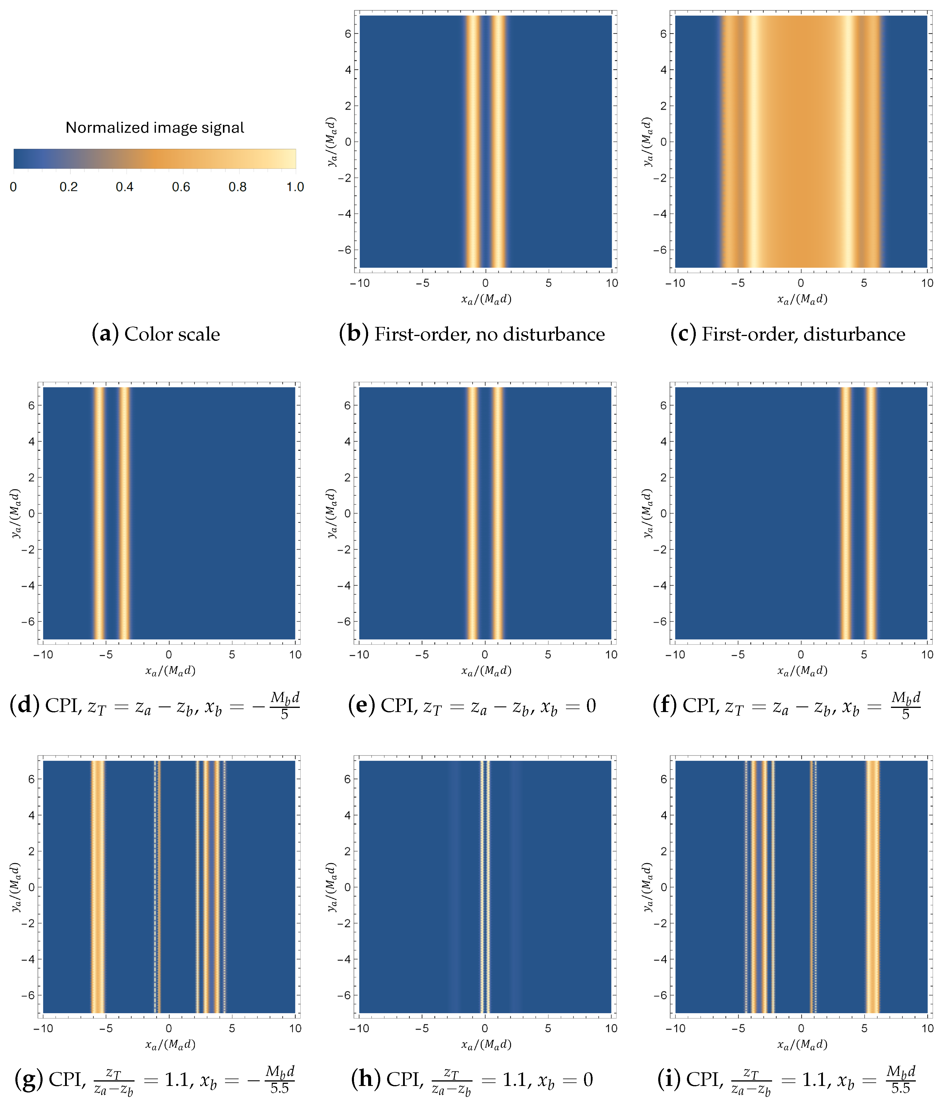
2. First-Order Imaging with an Axially Localized Turbulence

The optical scheme that we considered in this article, shown in Figure 1, is based on the paradigm of correlation plenoptic imaging between arbitrary planes (CPI-AP) [40]. It consists of a single lens of focal length f, that collects chaotic light of wavenumber k emitted by the object, placed at an arbitrary distance z, which undergoes turbulence at a distance $z_T$ on its way to the lens. After the lens, light is split into two paths by a beam splitter. The two beams impinge on the sensors ${\mathrm{D}}_a$ and ${\mathrm{D}}_b$, placed at distances $z_a^{\prime }$ and $z_b^{\prime }$, respectively. These two distances define two object planes at distances $z_a$ and $z_b$ in front of the lens, through the equations

$${\displaystyle \frac{1}{z_j}}+{\displaystyle \frac{1}{z_j^{\prime }}}={\displaystyle \frac{1}{f}},\mathrm{with}j=a,b.$$

(1)

The results here presented are based on the following assumptions on turbulence:

• Turbulence occurs upstream of the beam splitter, i.e., in the region where the optical paths are superposed.
• Turbulence is slowly varying in time and can be approximated as quasi-static in the time required to perform a reasonable reconstruction of the correlation function.
• Turbulence is due to unpredictable perturbations of the refractive index in a region of space of small longitudinal extension $\Delta z$, such that its effect amounts to multiplying the field in that region by a phase factor $exp(\mathrm{i}k\Delta n\left({\mathit{\rho }}_T\right)\Delta z)$, with ${\mathit{\rho }}_T$ the transverse coordinate of the turbulence plane and $\Delta n\left({\mathit{\rho }}_T\right)$ the change in refractive index with respect to the background. Notice, instead, that turbulence in a thick region should be described by a convolution of the field [57].

Figure 1. Optical scheme of the setup described in the article. Light from an object (the red arrow in figure), treated as a chaotic emitter, encounters turbulence in a thin region of space, at a distance $z_T$, before impinging on the lens. After the lens, light is split into two optical paths, impinging on the spatially-resolving sensors ${\mathrm{D}}_a$ and ${\mathrm{D}}_b$, respectively. The lens-to-sensor distances $z_j^{\prime }$, with $j=a,b$, define two object planes at the respective conjugate distances $z_j$, satisfying $1/z_j+1/z_j^{\prime }=1/f$, with f the focal length of the lens. The signal is collected by measuring pixel-by-pixel correlations between intensity fluctuations on the two sensors.

Figure 1. Optical scheme of the setup described in the article. Light from an object (the red arrow in figure), treated as a chaotic emitter, encounters turbulence in a thin region of space, at a distance $z_T$, before impinging on the lens. After the lens, light is split into two optical paths, impinging on the spatially-resolving sensors ${\mathrm{D}}_a$ and ${\mathrm{D}}_b$, respectively. The lens-to-sensor distances $z_j^{\prime }$, with $j=a,b$, define two object planes at the respective conjugate distances $z_j$, satisfying $1/z_j+1/z_j^{\prime }=1/f$, with f the focal length of the lens. The signal is collected by measuring pixel-by-pixel correlations between intensity fluctuations on the two sensors.

To explain the detrimental effect of turbulence, it is instructive to start from the first-order results, namely the intensity measured at the end of one of the optical paths. Neglecting, for the sake of simplicity, the finite aperture of the lens, the field propagator from an object point of coordinate ${\mathit{\rho }}_o$ and a point of coordinate ${\mathit{\rho }}_a$ on the sensor ${\mathrm{D}}_j$ reads

$$\begin{array}{c}{g}_j({\mathit{\rho }}_j,{\mathit{\rho }}_o)=C_j{\mathrm{e}}^{\mathrm{i}k\psi \left({\mathit{\rho }}_j\right)}exp\left({\displaystyle \frac{\mathrm{i}k{\mathit{\rho }}_o^2}{2z_T}}\right)\hfill \\ \hfill \times \int {\mathrm{d}}^2{\mathit{\rho }}_{T}exp\left\{\mathrm{i}k\left[\left({\displaystyle \frac{1}{z_T}}-{\displaystyle \frac{1}{z_T+z_j-z}}\right){\displaystyle \frac{{\mathit{\rho }}_T^2}{2}}-{\displaystyle \frac{{\mathit{\rho }}_T}{z_T}}·\left({\mathit{\rho }}_o+{\displaystyle \frac{z_T}{z_T+z_j-z}}{\displaystyle \frac{{\mathit{\rho }}_j}{M_j}}\right)-\varphi \left({\mathit{\rho }}_T\right)\right]\right\},\end{array}$$

(2)

where $\varphi \left({\mathit{\rho }}_T\right)=\Delta n\left({\mathit{\rho }}_T\right)\Delta z$ determines the phase change due to turbulence, and $M_j=z_j^{\prime }/z_j$, with $j=a,b$, are the absolute magnifications of the images focused by the lens on the two sensors. The above result is obtained by combining propagation through turbulence in $z_T$ with the transfer function $exp(-\mathrm{i}k{\mathit{\rho }}_{\ell }^2/2f)$ of the lens, where ${\mathit{\rho }}_{\ell }$ is the transverse coordinate on the lens plane, and with free-space propagation $exp[\mathrm{i}k{\left(\delta \mathit{\rho }\right)}^2/2\left(\delta z\right)]$, where $\delta \mathit{\rho }$ and $\delta z$ are the differences between transverse and axial coordinates, respectively [58]. If the object is a chaotic light emitter with intensity profile $\mathcal{A}\left({\mathit{\rho }}_o\right)$, the intensity measured on each sensor ${\mathrm{D}}_j$ reads

$$I_j\left({\mathit{\rho }}_j\right)=\int {\mathrm{d}}^2{\mathit{\rho }}_o\mathcal{A}\left({\mathit{\rho }}_o\right){\left|g_j({\mathit{\rho }}_j,{\mathit{\rho }}_o)\right|}^2.$$

(3)

In the case in which we are most interested when the object is focused on ${\mathrm{D}}_j$ (namely, $z=z_j$), the intensity reads, up to irrelevant constants,

$$I_j\left({\mathit{\rho }}_j\right)=\int {\mathrm{d}}^2{\mathit{\rho }}_o\mathcal{A}\left({\mathit{\rho }}_o\right){\left|\int {\mathrm{d}}^2{\mathit{\rho }}_{T}exp\left\{\mathrm{i}k\left[\varphi \left({\mathit{\rho }}_T\right)-{\displaystyle \frac{1}{z_T}}{\mathit{\rho }}_T·\left({\mathit{\rho }}_o+{\displaystyle \frac{{\mathit{\rho }}_j}{M_j}}\right)\right]\right\}\right|}^2,$$

(4)

leading to the stigmatic image $\mathcal{A}(-{\mathit{\rho }}_j/M_j)$, inverted and magnified by $M_j$, in the case of no turbulence. When turbulence is present, we can characterize its effect by considering the limit of geometrical optics $k\to \infty$, and the stationary-phase approximation [58], leading to

$$I_j\left({\mathit{\rho }}_j\right)\sim \int {\mathrm{d}}^2{\mathit{\rho }}_T\mathcal{A}\left(-{\displaystyle \frac{{\mathit{\rho }}_j}{M_j}}+z_T\nabla \varphi \left({\mathit{\rho }}_T\right)\right).$$

(5)

Therefore, in the presence of turbulence, rays passing from a point ${\rho }_T$ on the turbulence plane are deviated by an amount proportional to the gradient of the phase disturbance $\varphi$, leading to the superposition of sub-images characterized by different shifts. The disturbance is not directly determined by the phase perturbation, but rather by its gradient on the plane. This situation closely resembles the case of an out-of-focus object, which is commonly tackled by plenoptic imaging, with the relevant difference that, in the case of turbulence, the image shifts are unpredictable a priori. Notice that the effect of turbulence is less and less relevant as it occurs closer to the sample ($z_T\to 0$) since the spread due to turbulence at some point becomes less important than the natural point spread due to the finite lens aperture [55].

3. CPI for Turbulence Mitigation

Intuitively, as it occurs in CPI to reconstruct out-of-focus images, the detrimental effect of the superposition of shifted images in Equation (5) can be avoided if correlation measurement is able to detect each single sub-image with a well-defined shift, corresponding to a particular ${\mathit{\rho }}_T$. Therefore, let us consider the correlation function $\mathsf{\Gamma }({\mathit{\rho }}_a,{\mathit{\rho }}_b)$ between intensity fluctuations in a couple of points ${\mathit{\rho }}_a$ on the sensor ${\mathrm{D}}_a$ and ${\mathit{\rho }}_b$ on ${\mathrm{D}}_b$. Treating the object as a chaotic light emitter, as in Equation (3), one obtains

$$\mathsf{\Gamma }({\mathit{\rho }}_a,{\mathit{\rho }}_b)={\left|\int {\mathrm{d}}^2{\mathit{\rho }}_o\mathcal{A}\left({\mathit{\rho }}_o\right)g_a({\mathit{\rho }}_a,{\mathit{\rho }}_o)g_b^{\ast }({\mathit{\rho }}_b,{\mathit{\rho }}_o)\right|}^2.$$

(6)

Before treating the CPI-based reconstruction of the image, it is worth observing that the autocorrelation of intensity fluctuations

$$\mathsf{\Gamma }({\mathit{\rho }}_a,{\mathit{\rho }}_b)=I_a^2\left({\mathit{\rho }}_a\right)$$

(7)

coincides with the squared first-order intensity. This result could entail an apparent mitigation of turbulence in second-order measurement. However, the average result of the autocorrelation measurement is indistinguishable from measuring the intensity and squaring the result; therefore, effective mitigation occurs only if noise affecting $\mathsf{\Gamma }({\mathit{\rho }}_a,{\mathit{\rho }}_b)$ is lower than the one affecting $I_a^2\left({\mathit{\rho }}_a\right)$. This will be the object of future research.

Going back to the general form of $\mathsf{\Gamma }$, the result for the setup in Figure 1 can be evaluated by inserting the propagators defined in Equation (2), yielding, up to irrelevant constants,

$$\mathsf{\Gamma }({\mathit{\rho }}_a,{\mathit{\rho }}_b)={\left|\int {\mathrm{d}}^2{\mathit{\rho }}_o\int {\mathrm{d}}^2{\mathit{\rho }}_T\int {\mathrm{d}}^2{\mathit{\rho }}_T^{\prime }\mathcal{A}\left({\mathit{\rho }}_o\right)exp\left[\mathrm{i}k\mathsf{\Psi }({\mathit{\rho }}_a,{\mathit{\rho }}_b;{\mathit{\rho }}_o,{\mathit{\rho }}_T,{\mathit{\rho }}_T^{\prime })\right]\right|}^2,$$

(8)

where

$$\begin{array}{c}\mathsf{\Psi }({\mathit{\rho }}_a,{\mathit{\rho }}_b;{\mathit{\rho }}_o,{\mathit{\rho }}_T,{\mathit{\rho }}_T^{\prime })=\left({\displaystyle \frac{1}{z_T}}-{\displaystyle \frac{1}{z_T+z_a-z}}\right){\displaystyle \frac{{\mathit{\rho }}_T^2}{2}}-\left({\displaystyle \frac{1}{z_T}}-{\displaystyle \frac{1}{z_T+z_b-z}}\right){\displaystyle \frac{{{\mathit{\rho }}_T^{\prime }}^2}{2}}\hfill \\ \hfill -{\displaystyle \frac{1}{z_T}}{\mathit{\rho }}_o·({\mathit{\rho }}_T-{\mathit{\rho }}_T^{\prime })-{\displaystyle \frac{1}{z_T+z_a-z}}{\mathit{\rho }}_T·{\displaystyle \frac{{\mathit{\rho }}_a}{M_a}}+{\displaystyle \frac{1}{z_T+z_b-z}}{\mathit{\rho }}_T^{\prime }·{\displaystyle \frac{{\mathit{\rho }}_b}{M_b}}+\varphi \left({\mathit{\rho }}_T\right)-\varphi \left({\mathit{\rho }}_T^{\prime }\right).\end{array}$$

(9)

The stationary-phase conditions

$$\begin{array}{cc}\hfill {\nabla }_{{\mathit{\rho }}_0}\mathsf{\Psi }=& -{\displaystyle \frac{1}{z_T}}({\mathit{\rho }}_T-{\mathit{\rho }}_T^{\prime })=0,\hfill \end{array}$$

(10)

$$\begin{array}{cc}\hfill {\nabla }_{{\mathit{\rho }}_T}\mathsf{\Psi }=& \left({\displaystyle \frac{1}{z_T}}-{\displaystyle \frac{1}{z_T+z_a-z}}\right){\mathit{\rho }}_T-{\displaystyle \frac{1}{z_T}}{\mathit{\rho }}_o-{\displaystyle \frac{1}{z_T+z_a-z}}{\displaystyle \frac{{\mathit{\rho }}_a}{M_a}}+\nabla \varphi \left({\mathit{\rho }}_T\right)=0,\hfill \end{array}$$

(11)

$$\begin{array}{cc}\hfill {\nabla }_{{\mathit{\rho }}_T^{\prime }}\mathsf{\Psi }=& -\left({\displaystyle \frac{1}{z_T}}-{\displaystyle \frac{1}{z_T+z_b-z}}\right){\mathit{\rho }}_T^{\prime }+{\displaystyle \frac{1}{z_T}}{\mathit{\rho }}_o+{\displaystyle \frac{1}{z_T+z_b-z}}{\displaystyle \frac{{\mathit{\rho }}_b}{M_b}}-\nabla \varphi \left({\mathit{\rho }}_T^{\prime }\right)=0,\hfill \end{array}$$

(12)

that determine the point(s) $({\overline{\mathit{\rho }}}_o,{\overline{\mathit{\rho }}}_T,{\overline{\mathit{\rho }}}_T^{\prime })$ providing dominant contribution in the geometrical-optics limit $k\to \infty$, do not form a linear system in the integration variables, as would occur in the absence of turbulence, due to the presence of $\nabla \varphi$. However, the system is solvable anyway, as the equation that determines the stationary values of ${\mathit{\rho }}_T$ and ${\mathit{\rho }}_T^{\prime }$ is linear and independent of both ${\mathit{\rho }}_o$ and the phase variation gradient, leading to the solution

$${\overline{\mathit{\rho }}}_T={\overline{\mathit{\rho }}}_T^{\prime }={\displaystyle \frac{1}{z_a-z_b}}\left[(z_T+z_b-z){\displaystyle \frac{{\mathit{\rho }}_a}{M_a}}-(z_T+z_a-z){\displaystyle \frac{{\mathit{\rho }}_b}{M_b}}\right].$$

(13)

This enables to determine the stationary value of ${\mathit{\rho }}_o$ through the remaining independent condition, leading to

$${\overline{\mathit{\rho }}}_o=-{\displaystyle \frac{1}{z_a-z_b}}\left[(z-z_b){\displaystyle \frac{{\mathit{\rho }}_a}{M_a}}+(z_a-z){\displaystyle \frac{{\mathit{\rho }}_b}{M_b}}\right]+z_T\nabla \varphi \left({\overline{\mathit{\rho }}}_T\right).$$

(14)

Therefore, despite the turbulence, the dominant contribution to the correlation function comes from a single object point,

$$\begin{array}{c}\mathsf{\Gamma }({\mathit{\rho }}_a,{\mathit{\rho }}_b)\sim {\mathcal{A}}^2(-{\displaystyle \frac{1}{z_a-z_b}}\left[(z-z_b){\displaystyle \frac{{\mathit{\rho }}_a}{M_a}}+(z_a-z){\displaystyle \frac{{\mathit{\rho }}_b}{M_b}}\right]\hfill \\ \hfill \hspace{1em}\hspace{1em}\hspace{1em}\hspace{1em}\hspace{1em}\hspace{1em}\hspace{1em}\hspace{1em}\hspace{1em}+z_T\nabla \varphi \left({\displaystyle \frac{1}{z_a-z_b}}\left[(z_T+z_b-z){\displaystyle \frac{{\mathit{\rho }}_a}{M_a}}-(z_T+z_a-z){\displaystyle \frac{{\mathit{\rho }}_b}{M_b}}\right]\right)),\end{array}$$

(15)

providing a single shifted image for each pair of points $({\mathit{\rho }}_a,{\mathit{\rho }}_b)$. Clearly, this image is detectable only provided the time scale of turbulence is slow enough to permit the reconstruction of the correlation function with a reasonable signal-to-noise ratio. Specializing the result to the case of reference, in which the object is focused on ${\mathrm{D}}_a$ (for definiteness), with $z=z_a$, the correlation function takes the interesting form

$$\mathsf{\Gamma }({\mathit{\rho }}_a,{\mathit{\rho }}_b)\sim {\mathcal{A}}^2\left(-{\displaystyle \frac{{\mathit{\rho }}_a}{M_a}}+z_T\nabla \varphi \left({\displaystyle \frac{1}{z_a-z_b}}\left[(z_T+z_b-z_a){\displaystyle \frac{{\mathit{\rho }}_a}{M_a}}-z_T{\displaystyle \frac{{\mathit{\rho }}_b}{M_b}}\right]\right)\right).$$

(16)

A comparison with Equation (5) clarifies the potential of measuring pixel-by-pixel correlations across the two detectors instead of intensity: the choice of the pair $({\mathit{\rho }}_a,{\mathit{\rho }}_b)$ addresses a particular point ${\overline{\mathit{\rho }}}_T$ [see Equation (13)] on the turbulence plane, while intensity measurement erases such an information. At a fixed ${\mathit{\rho }}_b$, the image of the object is both shifted and distorted, due to the dependence on ${\mathit{\rho }}_a$ of the phase gradient. Incidentally, notice that the dependence of $\mathsf{\Gamma }$ on ${\mathit{\rho }}_b$ at a fixed ${\mathit{\rho }}_a$ can be used as an indicator to detect the presence of turbulence with a transverse gradient.

The correlation function in Equation (16) becomes particularly simple (and intuitive) when the turbulence plane is focused on ${\mathrm{D}}_b$, namely when $z_b=z_a-z_T$, where it reads

$$\mathsf{\Gamma }({\mathit{\rho }}_a,{\mathit{\rho }}_b)\sim {\mathcal{A}}^2\left(-{\displaystyle \frac{{\mathit{\rho }}_a}{M_a}}+z_T\nabla \varphi \left(-{\displaystyle \frac{{\mathit{\rho }}_b}{M_b}}\right)\right).$$

(17)

By varying ${\mathit{\rho }}_b$, one obtains a collection of images of the object, which are similar to each other up to a shift, as shown in Figure 2, where a comparison with first-order images is made. Once they are collected, one can evaluate their relative alignment (e.g., by computing the point-to-point correlation between them) and follow two strategies to obtain an integrated image, exploiting as much as possible the information contained in $\mathsf{\Gamma }({\mathit{\rho }}_a,{\mathit{\rho }}_b)$ and increasing the signal-to-noise ratio:

• sum only those sub-images characterized by the dominant alignment;
• realign all the sub-images with an alignment tool, and sum over them.

However, identifying the axial position of the turbulence plane can be challenging, and focusing the wrong plane on ${\mathrm{D}}_b$ can leave heavy distortion effects, as one can see in the bottom panels of Figure 2. Nonetheless, it is still possible to limit the effect of turbulence to a mere shift, by parametrizing the correlation function as

$$\mathsf{\Gamma }\left({\mathit{\rho }}_a,{\tilde{\mathit{\rho }}}_b({\mathit{\rho }}_a,{\overline{\mathit{\rho }}}_T)\right)\sim {\mathcal{A}}^2\left(-{\displaystyle \frac{{\mathit{\rho }}_a}{M_a}}+z_T\nabla \varphi \left({\overline{\mathit{\rho }}}_T\right)\right),$$

(18)

with

$${\tilde{\mathit{\rho }}}_b({\mathit{\rho }}_a,{\overline{\mathit{\rho }}}_T)=-{\displaystyle \frac{M_b}{z_T}}\left[{\overline{\mathit{\rho }}}_T+\left(1-{\displaystyle \frac{z_T}{z_a-z_b}}\right){\displaystyle \frac{{\mathit{\rho }}_a}{M_a}}\right].$$

(19)

If $z_T$ is unknown, it can be treated as a variational parameter, whose best estimate is the one that guarantees that all the images obtained at each fixed ${\mathit{\rho }}_b$ are similar up to a shift, as in Equation (18). Once it is determined, realignment of images can be made in the same way as in the case of Equation (17).

It is worth remembering that, due to the plenoptic properties of the correlation function, the advantage is not limited to the case of a focused object. However, though one can in principle reconstruct images of objects placed out of focus, wave-optics computation shows that the resolution of the correlation images is maximal in focus [36]. Here, resolution is determined by the Rayleigh limit, which is unattainable by traditional light-field techniques [36,42,43,59,60].

4. Discussion and Outlook

The results outlined in the previous section show that the light-field capability of CPI can be used to trace back the image of an object through phase disturbance by using intensity correlations to isolate the contribution of a limited area of the turbulence plane. Compared to analogous applications of standard light-field imaging to turbulence mitigation [20,47], CPI potentially provides diffraction-limited resolution on the focused plane and a much wider variety of independent viewpoints on a 3D sample [35]. Even though our analysis is limited to a focused object and to the geometrical-optics regime, recent wave-optics results demonstrated that the out-of-focus imaging properties of CPI entail a better volumetric resolution than any non-scanning first-order method [55].

One of the possible limitations of the method is related to the intrinsic need of CPI for collecting a large number of frames to provide a stable statistical reconstruction of the correlation function. Actually, the signal-to-noise ratio in correlation imaging is proportional to the square root of the number of collected frames, provided they are statistically independent of each other [31], as also confirmed by a recent experimental demonstration [44]. At the same time, increasing the duration of each frame beyond the coherence time of collected light tends to erase the signal [61]. To minimize the acquisition time while still achieving a satisfying signal-to-noise ratio, the duration of each frame must be as close as possible to the coherence time of collected light, while the dead time between two subsequent frames should be as small as possible. Moreover, if the phase disturbance is not constant, the total acquisition time must not exceed the typical variation time of the perturbation, to prevent frames corresponding to different phase gradients from contributing to the evaluation of the same correlation evaluation [see Equations (16) and (17)]. Therefore, the technique can largely benefit from new sensors that combine high-resolution with low noise (i.e., statistically reliable frames) and gating times close to the nanosecond [45,62,63,64], already applied to a CPI-AP experiment in a non-turbulent environment [44]. Moreover, especially in cases where time variation of turbulence does not allow achieving high signal-to-noise ratios, interesting developments can come from integrating the described methods with tools to maximize information extraction from data, like compressive sensing [65] and artificial intelligence [66], which can specifically help to realign noisy sub-images, even taken at different times.

The results presented in this article are relevant for cases in which the phase disturbance is concentrated in a small axial range compared to the optical baseline, and either static, such as irregular transparent surfaces, or varying at a rate that allows the capture of a CPI image (see [44]), such as localized heated air. Future research will be devoted to the analysis of phase disturbance effects on different methods of plenoptic imaging with intensity correlations, such as light-field ghost imaging [67]), and to extend the results to different models of turbulence. Specifically, we will consider the case in which phase disturbance is not static, and its effects pile up on a region of finite axial width, thus requiring more elaborated models of propagation through turbulence and the definition of time-averaged phase disturbance statistics [57].

References

1. Adelson, E.H.; Wang, J.Y. Single lens stereo with a plenoptic camera. IEEE Trans. Pattern Anal. Mach. Intell. 1992, 14, 99–106. [Google Scholar] [CrossRef]
2. Ng, R.; Levoy, M.; Brédif, M.; Duval, G.; Horowitz, M.; Hanrahan, P. Light field photography with a hand-held plenoptic camera. Comput. Sci. Tech. Rep. CSTR 2005, 2, 1–11. [Google Scholar]
3. Ng, R. Fourier slice photography. ACM Trans. Graph. 2005, 24, 735–744. [Google Scholar] [CrossRef]
4. Wu, G.; Masia, B.; Jarabo, A.; Zhang, Y.; Wang, L.; Dai, Q.; Chai, T.; Liu, Y. Light Field Image Processing: An Overview. IEEE J. Sel. Top. Signal Process. 2017, 11, 926–954. [Google Scholar] [CrossRef]
5. Lam, E.Y. Computational photography with plenoptic camera and light field capture: Tutorial. J. Opt. Soc. Am. A 2015, 32, 2021–2032. [Google Scholar] [CrossRef] [PubMed]
6. Mertz, J. Introduction to Optical Microscopy; Cambridge University Press: Cambridge, UK, 2019. [Google Scholar]
7. Huisken, J.; Swoger, J.; Del Bene, F.; Wittbrodt, J.; Stelzer, E.H.K. Optical sectioning deep inside live embryos by selective plane illumination microscopy. Science 2004, 305, 1007. [Google Scholar] [CrossRef] [PubMed]
8. Fahrbach, F.O.; Simon, P.; Rohrbach, A. Microscopy with self-reconstructing beams. Nat. Photonics 2010, 4, 780. [Google Scholar] [CrossRef]
9. Vettenburg, T.; Dalgarno, H.I.C.; Nylk, J.; Coll-Lladó, C.; Ferrier, D.E.K.; Čižmár, T.; Gunn-Moore, F.J.; Dholakia, K. Light-sheet microscopy using an Airy beam. Nat. Methods 2014, 11, 541–544. [Google Scholar] [CrossRef] [PubMed]
10. Hall, E.M.; Thurow, B.S.; Guildenbecher, D.R. Comparison of three-dimensional particle tracking and sizing using plenoptic imaging and digital in-line holography. Appl. Opt. 2016, 55, 6410–6420. [Google Scholar] [CrossRef]
11. Levoy, M.; Ng, R.; Adams, A.; Footer, M.; Horowitz, M. Light field microscopy. ACM Trans. Graph. (TOG) 2006, 25, 924. [Google Scholar] [CrossRef]
12. Broxton, M.; Grosenick, L.; Yang, S.; Cohen, N.; Andalman, A.; Deisseroth, K.; Levoy, M. Wave optics theory and 3-D deconvolution for the light field microscope. Opt. Express 2013, 21, 25418. [Google Scholar] [CrossRef]
13. Glastre, W.; Hugon, O.; Jacquin, O.; de Chatellus, H.G.; Lacot, E. Demonstration of a plenoptic microscope based on laser optical feedback imaging. Opt. Express 2013, 21, 7294. [Google Scholar] [CrossRef] [PubMed]
14. Prevedel, R.; Yoon, Y.G.; Hoffmann, M.; Pak, N.; Wetzstein, G.; Kato, S.; Schrödel, T.; Raskar, R.; Zimmer, M.; Boyden, E.S.; et al. Simultaneous whole-animal 3D imaging of neuronal activity using light-field microscopy. Nat. Methods 2014, 11, 727. [Google Scholar] [CrossRef]
15. Muenzel, S.; Fleischer, J.W. Enhancing layered 3D displays with a lens. Appl. Opt. 2013, 52, D97. [Google Scholar] [CrossRef] [PubMed]
16. Levoy, M.; Hanrahan, P. Light field rendering. In Proceedings of the 23rd Annual Conference on Computer Graphics and Interactive Techniques, New Orleans, LA, USA, 4–9 August 1996; ACM: New York, NY, USA, 1996; pp. 31–42. [Google Scholar]
17. Wu, C. The Plenoptic Sensor. Ph.D. Thesis, University of Maryland, College Park, MD, USA, 2016. [Google Scholar]
18. Lv, Y.; Wang, R.; Ma, H.; Zhang, X.; Ning, Y.; Xu, X. SU-G-IeP4-09: Method of Human Eye Aberration Measurement Using Plenoptic Camera over Large Field of View. Med. Phys. 2016, 43, 3679. [Google Scholar] [CrossRef]
19. Wu, C.; Ko, J.; Davis, C.C. Using a plenoptic sensor to reconstruct vortex phase structures. Opt. Lett. 2016, 41, 3169. [Google Scholar] [CrossRef]
20. Wu, C.; Ko, J.; Davis, C.C. Imaging through strong turbulence with a light field approach. Opt. Express 2016, 24, 11975. [Google Scholar] [CrossRef] [PubMed]
21. Ko, J.; Davis, C.C. Comparison of the plenoptic sensor and the Shack–Hartmann sensor. Appl. Opt. 2017, 56, 3689–3698. [Google Scholar] [CrossRef]
22. Fahringer, T.W.; Lynch, K.P.; Thurow, B.S. Volumetric particle image velocimetry with a single plenoptic camera. Meas. Sci. Technol. 2015, 26, 115201. [Google Scholar] [CrossRef]
23. Skocek, O.; Noebauer, T.; Weilguny, L.; Martínez Traub, F.; Xia, C.; Molodtsov, M.; Grama, A.; Yamagata, M.; Aharoni, D.; Cox, D.; et al. High-speed volumetric imaging of neuronal activity in freely moving rodents. Nat. Methods 2018, 15, 429–432. [Google Scholar] [CrossRef]
24. Xiao, X.; Javidi, B.; Martinez-Corral, M.; Stern, A. Advances in three-dimensional integral imaging: Sensing, display, and applications [Invited]. Appl. Opt. 2013, 52, 546. [Google Scholar] [CrossRef] [PubMed]
25. Georgiev, T.G.; Lumsdaine, A. Focused plenoptic camera and rendering. J. Electron. Imaging 2010, 19, 021106. [Google Scholar]
26. Pittman, T.B.; Shih, Y.H.; Strekalov, D.V.; Sergienko, A.V. Optical imaging by means of two-photon quantum entanglement. Phys. Rev. A 1995, 52, R3429. [Google Scholar] [CrossRef] [PubMed]
27. Bennink, R.S.; Bentley, S.J.; Boyd, R.W. “Two-photon” coincidence imaging with a classical source. Phys. Rev. Lett. 2002, 89, 113601. [Google Scholar] [CrossRef] [PubMed]
28. Valencia, A.; Scarcelli, G.; D’Angelo, M.; Shih, Y. Two-photon imaging with thermal light. Phys. Rev. Lett. 2005, 94, 063601. [Google Scholar] [CrossRef] [PubMed]
29. Gatti, A.; Brambilla, E.; Bache, M.; Lugiato, L.A. Ghost imaging with thermal light: Comparing entanglement and classical correlation. Phys. Rev. Lett. 2004, 93, 093602. [Google Scholar] [CrossRef] [PubMed]
30. Scarcelli, G.; Berardi, V.; Shih, Y. Can two-photon correlation of chaotic light be considered as correlation of intensity fluctuations? Phys. Rev. Lett. 2006, 96, 063602. [Google Scholar] [CrossRef] [PubMed]
31. O’Sullivan, M.N.; Chan, K.W.C.; Boyd, R.W. Comparison of the signal-to-noise characteristics of quantum versus thermal ghost imaging. Phys. Rev. A 2010, 82, 053803. [Google Scholar] [CrossRef]
32. Brida, G.; Chekhova, M.; Fornaro, G.; Genovese, M.; Lopaeva, E.; Berchera, I.R. Systematic analysis of signal-to-noise ratio in bipartite ghost imaging with classical and quantum light. Phys. Rev. A 2011, 83, 063807. [Google Scholar] [CrossRef]
33. Cassano, M.; D’Angelo, M.; Garuccio, A.; Peng, T.; Shih, Y.; Tamma, V. Spatial interference between pairs of disjoint optical paths with a chaotic source. Opt. Express 2017, 25, 6589–6603. [Google Scholar] [CrossRef]
34. D’Angelo, M.; Mazzilli, A.; Pepe, F.V.; Garuccio, A.; Tamma, V. Characterization of two distant double-slits by chaotic light second-order interference. Sci. Rep. 2017, 7, 2247. [Google Scholar] [CrossRef] [PubMed]
35. D’Angelo, M.; Pepe, F.V.; Garuccio, A.; Scarcelli, G. Correlation plenoptic imaging. Phys. Rev. Lett. 2016, 116, 223602. [Google Scholar] [CrossRef] [PubMed]
36. Pepe, F.V.; Di Lena, F.; Mazzilli, A.; Edrei, E.; Garuccio, A.; Scarcelli, G.; D’Angelo, M. Diffraction-limited plenoptic imaging with correlated light. Phys. Rev. Lett. 2017, 119, 243602. [Google Scholar] [CrossRef] [PubMed]
37. Pepe, F.V.; Scarcelli, G.; Garuccio, A.; D’Angelo, M. Plenoptic imaging with second-order correlations of light. Quantum Meas. Quantum Metrol. 2016, 3, 20. [Google Scholar] [CrossRef]
38. Pepe, F.V.; Di Lena, F.; Garuccio, A.; Scarcelli, G.; D’Angelo, M. Correlation Plenoptic Imaging with Entangled Photons. Technologies 2016, 4, 17. [Google Scholar] [CrossRef]
39. Pepe, F.V.; Vaccarelli, O.; Garuccio, A.; Scarcelli, G.; D’Angelo, M. Exploring plenoptic properties of correlation imaging with chaotic light. J. Opt. 2017, 19, 114001. [Google Scholar] [CrossRef]
40. Di Lena, F.; Massaro, G.; Lupo, A.; Garuccio, A.; Pepe, F.V.; D’Angelo, M. Correlation plenoptic imaging between arbitrary planes. Opt. Express 2020, 28, 35857–35868. [Google Scholar] [CrossRef] [PubMed]
41. Scagliola, A.; Di Lena, F.; Garuccio, A.; D’Angelo, M.; Pepe, F.V. Correlation Plenoptic Imaging for microscopy applications. Phys. Lett. A 2020, 384, 126472. [Google Scholar] [CrossRef]
42. Massaro, G.; Di Lena, F.; D’Angelo, M.; Pepe, F.V. Effect of Finite-Sized Optical Components and Pixels on Light-Field Imaging through Correlated Light. Sensors 2022, 22, 2778. [Google Scholar] [CrossRef] [PubMed]
43. Massaro, G.; Pepe, F.V.; D’Angelo, M. Refocusing Algorithm for Correlation Plenoptic Imaging. Sensors 2022, 22, 6665. [Google Scholar] [CrossRef]
44. Massaro, G.; Mos, P.; Vasiukov, S.; Di Lena, F.; Scattarella, F.; Pepe, F.V.; Ulku, A.; Giannella, D.; Charbon, E.; Bruschini, C.; et al. Correlated-photon imaging at 10 volumetric images per second. Sci. Rep. 2023, 13, 12813. [Google Scholar] [CrossRef] [PubMed]
45. Abbattista, C.; Amoruso, L.; Burri, S.; Charbon, E.; Di Lena, F.; Garuccio, A.; Giannella, D.; Hradil, Z.; Iacobellis, M.; Massaro, G.; et al. Towards Quantum 3D Imaging Devices. Appl. Sci. 2021, 11, 6414. [Google Scholar] [CrossRef]
46. Michael, C.R.; Byron, M.W. Imaging through Turbulence; CRC Press: Boca Raton, FL, USA, 1996. [Google Scholar]
47. Wu, C.; Ko, J.; Davis, C.C. Imaging Through Turbulence Using a Plenoptic Sensor. Proc. SPIE 2015, 9614, 961405. [Google Scholar]
48. Cheng, J. Ghost imaging through turbulent atmosphere. Opt. Express 2009, 17, 7916–7921. [Google Scholar] [CrossRef] [PubMed]
49. Li, C.; Wang, T.; Pu, J.; Zhu, W.; Rao, R. Ghost imaging with partially coherent light radiation through turbulent atmosphere. Appl. Phys. B 2010, 99, 599–604. [Google Scholar] [CrossRef]
50. Chan, K.W.C.; Simon, D.S.; Sergienko, A.V.; Hardy, N.D.; Shapiro, J.H.; Dixon, P.B.; Howland, G.A.; Howell, J.C.; Eberly, J.H.; O’Sullivan, M.; et al. Theoretical analysis of quantum ghost imaging through turbulence. Phys. Rev. A 2011, 84, 043807. [Google Scholar] [CrossRef]
51. Hardy, N.D.; Shapiro, J.H. Reflective ghost imaging through turbulence. Phys. Rev. A 2011, 84, 063824. [Google Scholar] [CrossRef]
52. Dixon, P.B.; Howland, G.A.; Chan, K.W.C.; O’Sullivan-Hale, C.; Rodenburg, B.; Hardy, N.D.; Shapiro, J.H.; Simon, D.S.; Sergienko, A.V.; Boyd, R.W.; et al. Quantum ghost imaging through turbulence. Phys. Rev. A 2011, 83, 051803. [Google Scholar] [CrossRef]
53. Meyers, R.E.; Deacon, K.S.; Shih, Y. Turbulence-free ghost imaging. Appl. Phys. Lett. 2011, 98, 111115. [Google Scholar] [CrossRef]
54. Shi, D.; Fan, C.; Zhang, P.; Zhang, J.; Shen, H.; Qiao, C.; Wang, Y. Adaptive optical ghost imaging through atmospheric turbulence. Opt. Express 2012, 20, 27992–27998. [Google Scholar] [CrossRef]
55. Massaro, G.; Giannella, D.; Scagliola, A.; Di Lena, F.; Scarcelli, G.; Garuccio, A.; Pepe, F.V.; D’Angelo, M. Light-field microscopy with correlated beams for extended volumetric imaging at the diffraction limit. Sci. Rep. 2022, 12, 16823. [Google Scholar] [CrossRef] [PubMed]
56. Massaro, G. Assessing the 3D resolution of refocused correlation plenoptic images using a general-purpose image quality estimator. arXiv 2024, arXiv:2406.13501. [Google Scholar]
57. Fante, R.L. Wave propagation in random media: A systems approach. In Progress in Optics XXII; Wolf, E., Ed.; Elsevier: Amsterdam, The Netherlands, 1985; pp. 343–398. [Google Scholar]
58. Saleh, B.E.A.; Teich, M.C. Fundamentals of Photonics; John Wiley & Sons: New York, NY, USA, 2007. [Google Scholar]
59. Scattarella, F.; D’Angelo, M.; Pepe, F.V. Resolution Limit of Correlation Plenoptic Imaging between Arbitrary Planes. Optics 2022, 3, 138–149. [Google Scholar] [CrossRef]
60. Scattarella, F.; Massaro, G.; Stoklasa, B.; D’Angelo, M.; Pepe, F.V. Periodic patterns for resolution limit characterization of correlation plenoptic imaging. Eur. Phys. J. Plus 2023, 138, 710. [Google Scholar] [CrossRef]
61. Mandel, L.; Wolf, E. Optical Coherence and Quantum Optics; Cambridge University Press: Cambridge, UK, 1995. [Google Scholar]
62. Antolovic, I.M.; Burri, S.; Hoebe, R.A.; Maruyama, Y.; Bruschini, C.; Charbon, E. Photon-counting arrays for time-resolved imaging. Sensors 2016, 16, 1005. [Google Scholar] [CrossRef] [PubMed]
63. Lubin, G.; Tenne, R.; Antolovic, I.M.; Charbon, E.; Bruschini, C.; Oron, D. Quantum correlation measurement with single photon avalanche diode arrays. Opt. Express 2019, 27, 32863–32882. [Google Scholar] [CrossRef] [PubMed]
64. Ulku, A.C.; Ardelean, A.; Antolovic, I.M.; Weiss, S.; Charbon, E.; Bruschini, C.; Michalet, X. Wide-field time-gated SPAD imager for phasor-based FLIM applications. Methods Appl. Fluoresc. 2020, 98, 024002. [Google Scholar] [CrossRef] [PubMed]
65. Petrelli, I.; Santoro, F.; Massaro, G.; Scattarella, F.; Pepe, F.V.; Mazzia, F.; Ieronymaki, M.; Filios, G.; Mylonas, D.; Pappas, N.; et al. Compressive sensing-based correlation plenoptic imaging. Front. Phys. 2023, 11, 1287740. [Google Scholar] [CrossRef]
66. Scattarella, F.; Diacono, D.; Monaco, A.; Amoroso, N.; Bellantuono, L.; Massaro, G.; Pepe, F.V.; Tangaro, S.; Bellotti, R.; D’Angelo, M. Deep learning approach for denoising low-SNR correlation plenoptic images. Sci. Rep. 2023, 13, 19645. [Google Scholar] [CrossRef]
67. Paniate, A.; Massaro, G.; Avella, A.; Meda, A.; Pepe, F.V.; Genovese, M.; D’Angelo, M.; Ruo-Berchera, I. Light-field ghost imaging. Phys. Rev. Appl. 2024, 21, 024032. [Google Scholar] [CrossRef]
Figure 2. Imaging of two parallel slits, at a relative distance 2 d , through a static phase disturbance, axially localized in z T , and varying only along the direction (x) orthogonal to the slits, with profile ϕ ( x T ) = ( d / z T ) cos 2 ( 5 x T / a ) . Panel (a) shows the common color scale of the reported image signals (either intensity or correlation). Panels (b,c) contain first-order images, obtained without and with phase disturbance, respectively, [see Equation (5)]. Panels (df) illustrate the correlation function Γ ( ρ a , ρ b ) taken at different fixed values of x b (while y b = 0 in all cases), when the turbulence plane is focused on the sensor D b ; the cases in panels (d,f) are among the most affected by turbulence-related shift [see Equation (17)]. Panels (gi) illustrate the correlation function Γ ( ρ a , ρ b ) taken at different fixed values of x b (while y b = 0 in all cases), when the turbulence plane is not focused on the sensor D b ; besides being shifted, all the images are also affected by distortion, as in the general case of Equation (16), and require the reparametrization in Equations (18) and (19) to reconstruct faithful images. The slits have a Gaussian intensity transmission profile of width d / s q r t 8 , while the finite size of the lens is assumed to be negligible for simplicity.
Photonics 11 00733 g002
Disclaimer/Publisher’s Note: The statements, opinions and data contained in all publications are solely those of the individual author(s) and contributor(s) and not of MDPI and/or the editor(s). MDPI and/or the editor(s) disclaim responsibility for any injury to people or property resulting from any ideas, methods, instructions or products referred to in the content.