Article

Improving the Performances of Optical Tweezers by Using Simple Binary Diffractive Optics

by
Kamel Aït-Ameur
1,* and
Abdelkrim Hasnaoui
2
1
Centre de Recherche sur les Ions, Les Matériaux et la Photonique (CIMAP), UMR 6252 CEA-CNRS-ENSICAEN-Université de Caen, 6 Bd Maréchal Juin, CEDEX 4, 14050 Caen, France
2
Institut National d’Optométrie d’Ouled Fayet (INOOF), Résidence Les Palmiers, RW233, Ouled Fayet Algiers, Algeria
*
Author to whom correspondence should be addressed.
Photonics 2024, 11(8), 744; https://doi.org/10.3390/photonics11080744
Submission received: 16 July 2024 / Revised: 4 August 2024 / Accepted: 5 August 2024 / Published: 8 August 2024
(This article belongs to the Section Lasers, Light Sources and Sensors)

Abstract

:
Usually, optical tweezers for trapping atoms or nanoparticles are based on the focusing of a Gaussian laser beam (GB). The optical trap is characterised by its longitudinal stability (LS), expressed as the ratio of the backward axial gradient and the forward scattering forces. Replacing the GB with a LGp0 beam (one central peak surrounded by p rings) does not improve the LS because the on-axis intensity distribution is the same whatever the mode order p. However, it has been recently demonstrated that a restructured LGp0 beam can improve greatly the LS. In this paper, we consider the restructuring of a LGp0 beam when passing through a simple binary diffracting optical element called a circular π-plate (CPP). For a particular radius of the dephasing zone of the CPP, it is found that the LS is multiplied by a factor corresponding to a relative increase of about 220% to 320%.

1. Introduction

It is commonly admitted that the focusing of a Gaussian beam in the presence of a positive spherical aberration (SA) leads to a degraded focus characterised by a reduced intensity in the focal plane [1,2], and reduced longitudinal and radial intensity gradients [3]. The main characteristic of an optical trap is its longitudinal stability (LS), expressed as the ratio of the backward axial gradient and the forward scattering forces. The challenge in this work is to illuminate the optical tweezers with a restructured (non-Gaussian) laser beam in order to make the LS as high as possible for a given laser beam power, and consequently performing better than the usual Gaussian beam. It is generally agreed that spherical aberrations and optical tweezers illuminated by a Gaussian beam do not mix too well. The question of improving the tweezers’ performance through its illumination by a structured laser beam not necessarily Gaussian has long been considered. The most recent results are as follows:
(a)
The trap is illuminated by a rectified LGp0 beam [4]. Let us recall that a radial Laguerre–Gauss LGp0 beam is made up of a central peak surrounded by p rings alternately positive and negative. The beam rectification is obtained by inserting a binary diffractive optical element made up of concentric dephasing zones making all the rings to be positive. The longitudinal force is improved by a factor ranging from (p + 1) to (p + 2). In contrast, the radial force is not improved.
(b)
The second possibility is based on the addition of an optical Kerr effect while focusing the Gaussian beam illuminating the trap [5,6]. Doing that improves the longitudinal force by a factor of not more than two for particular values of the input power [6].
(c)
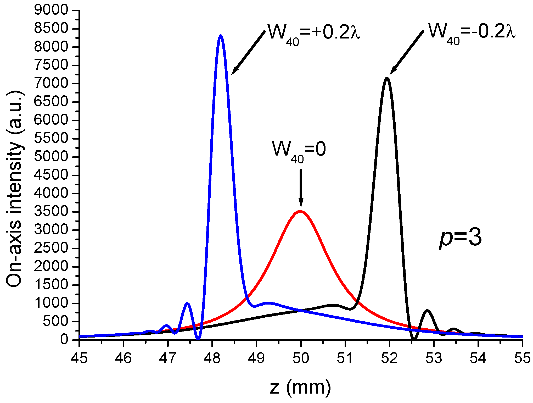
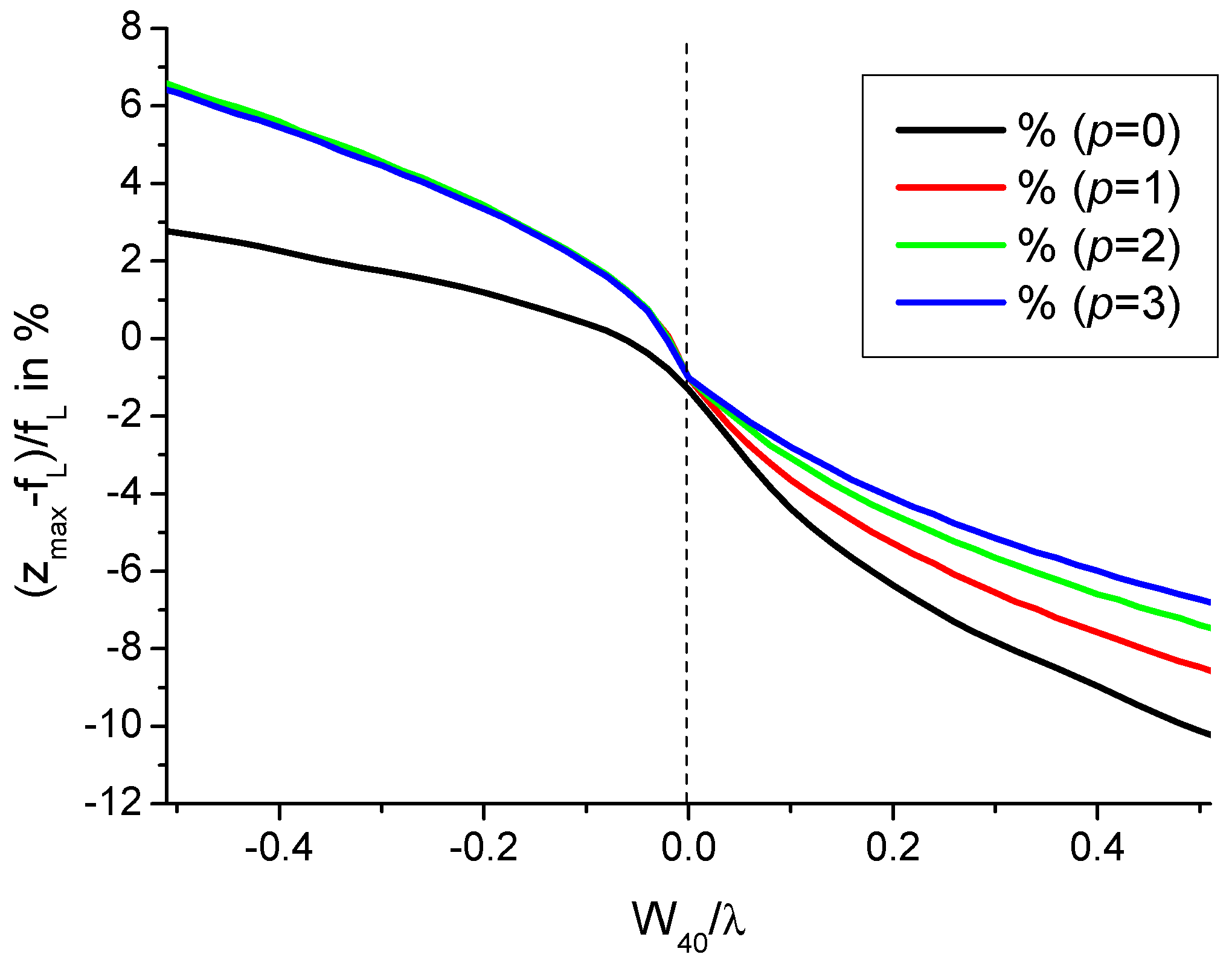
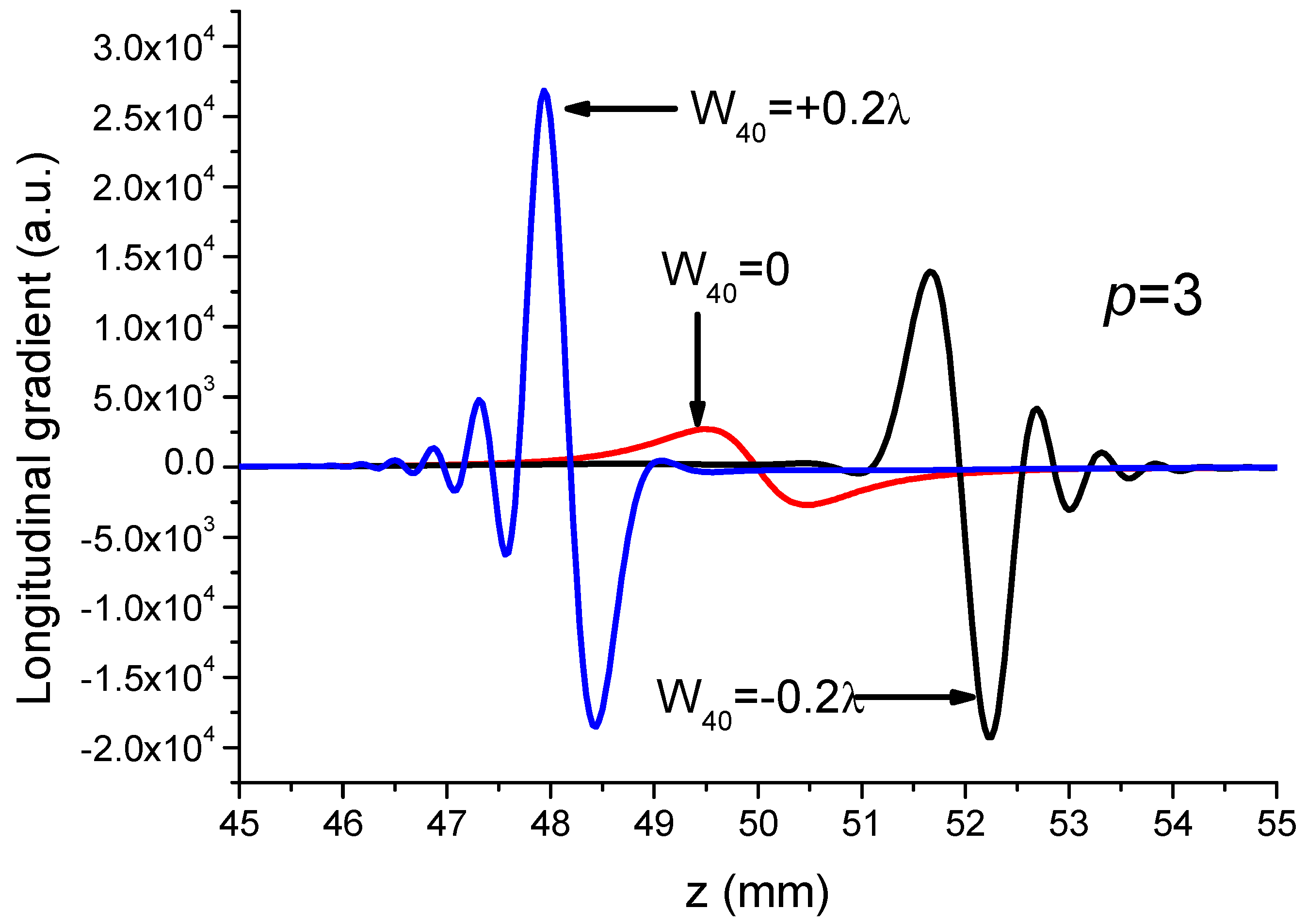
The third possibility is to introduce a primary or secondary spherical aberration on the path of the incident LGp0 beam. This allows for increasing several times both the longitudinal and transverse trapping effect for a given incident power [3] especially if the spherical aberration is negative.
Note that replacing the usual Gaussian beam by a pure LGp0 beam, for a given power, does not improve the longitudinal force of the trap because the on-axis intensity distribution remains the same whatever the mode order p. It just improves slightly the radial force because the width of the central peak decreases with p [3,7]. In order to enhance the longitudinal force, it is necessary to structure the incident LGp0 beam by setting an adequate phase aberration profile (PAP) φ ( ρ ) , as shown in Figure 1, and where ρ is the radial coordinate. The main points of the theory of optical tweezers can be found in Appendix A, and more details are available in [8,9,10,11,12,13]. It is assumed that the optical trap is in the Rayleigh regime for which the size of the trapped particle is very small compared to the wavelength. Consequently, even focused, the LGp0 beam can be reduced to its main central peak in consideration of the particle size.
Figure 1 shows the problematic of improving the capacity of trapping of optical tweezers by structuring the incident laser beam by the use of a phase aberration profile (PAP) φ ( ρ ) . Recently, it has been demonstrated that when φ ( ρ ) takes the form of a primary or secondary spherical aberration, it is possible to greatly enhance the longitudinal and radial forces [3]. It is convenient to use the figures of merit Z L (see the Appendix A) in order to measure the factor by which the longitudinal stability (LS) is multiplied in the presence of the PAP φ ( ρ ) . When Z L is greater (smaller) than unity it can be argued that the trap performance has been improved (reduced).

2. Optical Tweezers Illuminated by a L G p 0 Beam Subject to Spherical Aberration

The complex transmittance τ φ of the PAP φ ( ρ ) is given by
τ φ = exp [ i φ ( ρ ) ]
An interesting case is when the phase aberration profile φ ( ρ ) is a spherical aberration φ S A ( ρ ) taking different forms depending on integer N:
φ ( ρ ) = φ S A ( ρ ) = k W N 0 ρ ρ 0 N
N = 4 stands for the primary SA, N = 6 for the secondary SA. W N 0 is the primary and secondary spherical aberration coefficient. The quantity ρ 0 represents the radius of the unit circle which, by definition, contains 99.9% of the incident power. Table 1 gives the variations in ρ 0 with the incident mode order p.
The incident collimated radial Laguerre–Gaussian L G p 0 beam of order p is characterised by its amplitude electric field distribution E i n ( ρ ) given by
E i n ( ρ ) = E 0 L p ( 2 ρ 2 / W 2 ) exp ( ρ 2 / W 2 )
where W = 1 mm is the width of the Gaussian beam (p = 0), and L p is the Laguerre polynomial. The power carried by the L G p 0 beam is equal to P i n = π W 2 E 0 2 / 2 and is the same whatever the mode order p. The complex transmittance τ L of the focusing lens of focal length fL = 50 mm is given by
τ L = exp i k ρ 2 2 f L
The calculus of Z L (see Appendix A) is based on the intensity distribution I d ( r , z ) = E d ( r , z ) 2 , where E d ( r , z ) is the diffracted field associated with the beam emerging from the ensemble (lens + PAP) given by the Fresnel–Kirchhoff integral:
E d ( r , z ) = 2 π λ z 0 τ L ( ρ ) τ φ ( ρ ) E i n ( ρ ) exp i π ρ 2 λ 1 f L 1 z J 0 2 π λ z r . ρ ρ d ρ
where r (ρ) is the radial coordinate in the plane z (Lens + PAP) and J 0 is the zero-order Bessel function of first order. The integral given by Equation (5) is calculated by using a FORTRAN routine based on the numerical integrator dqdag from the International Mathematics and Statistical Library (IMSL).
Remark: The calculation of Z L is made for a focusing lens of focal length fL = 50 mm which is unusual for optical tweezers because it does not allow to achieve a tight focusing. The main reasons for this choice are for ensuring a validity of the Fresnel–Kirchhoff integral which could be questionable for a very short focal length f L , and for maintaining a certain continuity with our previous works [3,4,6].
The variations in Z L versus the aberration coefficients W 40 and W 60 have been already considered in [3] for a W N 0 varying from λ / 10 to + λ / 10 . Here, we emphasise only the effect of a primary SA on the performances of an optical trap illuminated by a L G p 0 beam, but on a greater range of W 40 values, i.e., from λ to + λ .
Figure 2 shows that in presence of a spherical aberration, the longitudinal stability of the optical trap illuminated by a L G p 0 beam (with p >0) can be increased significantly, especially when W 40 is negative. It is also seen in Figure 2 that when the trap is illuminated by a Gaussian L G 00 beam the longitudinal stability is essentially degraded in the presence of a spherical aberration, except for a small range of negative coefficient W 40 for which Z L is slightly improved. For a higher-order p, the maximum value reached by the figure of merit Z L is of order (p + 2). The results shown in Figure 2 would appear at first sight relatively surprising since usually users of optical tweezers illuminated by a Gaussian beam do everything to reduce or compensate the SA originating from the usual glass substrate forming part of the optical tweezers, which introduces a refractive index mismatch with respect to the surrounding medium [14,15,16,17,18]. In fact, what we recently showed [3] is that the effect of a spherical aberration on the performance of optical tweezers illuminated not by a Gaussian beam but by a high-order L G p 0 beam (p > 0) enhances its performances, i.e., Z L > 1 , as shown in Figure 2.
Figure 3 shows that there are at least two effects when the L G 30 beam, for instance, to be focused is subject to a spherical aberration. The first one is a shift of the best focus, i.e., the maximum of intensity, beyond (before) the focal plane z = f L when W 40 is negative (positive). The second one is a substantial strengthening of the maximum of intensity accompanied by a gradient stiffening. The shift of the best focus position could be understood by having recourse to a mean focal length f 40 given by [19], characterising the lensing effect associated with the SA:
f 40 ρ 0 2 4 3 λ W 40
It is important to note that the spherical aberration cannot be reduced to a simple lensing effect having regard to the height of the on-axis intensity maximum for W 40 < 0 . Indeed, the on-axis intensity maximum should have been reduced with respect to the case W 40 = 0 for a pure lensing effect. Another point of view justifying that we are not dealing with a pure lensing effect associated with the SA is to consider the variations in the position z max of the best focus versus W 40 . Indeed, the plots in Figure 4 show that the focus shift is dependent (independent) on mode order p 1 for positive (negative) spherical aberration; the case p = 0 having once again a specific behaviour as mentioned above. Note that the values of ( z max f L ) / f L in Figure 4 are slightly different from those given in [3] because the values of the unit circle radius ρ 0 are different. Consequently, one can deduce that the spherical aberration has an action of restructuring the laser beam by a transfer of energy from the surrounding rings towards the central peak.
The plots in Figure 5 show that the presence of the spherical aberration enhances the longitudinal gradient of the on-axis intensity which permits an understanding of the improvement in the LS shown in Figure 2. As introduced in the Appendix A, the optical trap is characterised by the longitudinal position z min where the gradient force can overcome the scattering force. More simply, one can say that the trapping position of the particle is z min which varies with the spherical aberration as shown in Figure 6. In contrast to what is seen in Figure 4, the value of z min is dependent (independent) on mode order p 1 for negative (positive) spherical aberration; the case p = 0 has always a specific behaviour.
In the next Section we will consider the use of simple diffractive optics described in terms of a mixing of primary, secondary and tertiary spherical aberrations [20], and allowing for implementing an adjustable, in sign and value, spherical aberration.

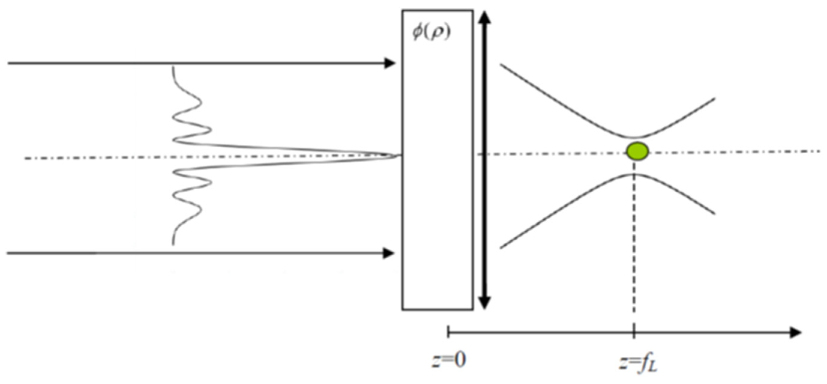
3. Restructuring the Laser Beam Illuminating the Tweezers

As seen previously, it is possible to enhance the LS of optical tweezers by using a L G p 0 laser beam subject to spherical aberration (SA) for its illumination. The order of magnitude of the factor which multiplies the ratio F g r a d / F s c a t is equal to about (p + 2), provided that the SA coefficient W 40 takes an adequate value as seen in Figure 2. Let us pass now to the implementation of the spherical aberration by examining the different possibilities.
The most practical way for generating a wavefront having the adequate shape so that it carries a specific spherical aberration could be the use of a spatial light modulator (SLM) [21], or a deformable mirror (DM) [22]. Although these solutions are elegant and powerful, they are also very expensive, and a cheaper one is desirable. For that, there are at least two possible solutions. The first one consists of the use of the spherical aberration associated with a thin converging or diverging lens according to the desired SA sign. A.E. Siegman [23] proposed a simple modelling allowing the determination of the desired W 40 coefficient resulting from a thin lens having a focal length f:
W 40 = C 4 ρ 0 4 f 3
where C 4 f is a dimensionless factor that is typically equal to one [23]. For instance, if we desire an aberration coefficient W 40 = 0.2 λ , then f ≈ −42 mm for a unit circle radius ρ0 = 2 mm. Such a diverging lens would not disturb significantly the quality of the tight focusing carried out by a focusing lens of very short focal length (some millimetres). This solution, unfortunately, does not provide the opportunity to allow easy and quick adjustments of W 40 .
The second possibility for generating a negative SA ( W 40   <   0 ) consists of using the diffractive aberration originating from a binary diffractive optical element (BDOE) made up of a circular π-plate (CPP), as shown recently [20]. Before proceeding, let us recall that a CPP is a BDOE which introduces a π-phase shift in the central region of the incident laser beam. The CPP is characterised by its complex transmittance τ C given by
τ C ( ρ ) = 1   f o r   ρ R P I + 1   f o r   ρ > R P I
The formalism used for the calculation of the aberration coefficients A j can be found in [24,25], and recalled briefly in Appendix B. As shown in Figure A3, the spherical aberration coefficients can be positive or negative depending on the radius R P I of the CPP. Consequently, it would be interesting to replace the phase aberration φ ( ρ ) shown in Figure 1 with a CPP, and to check if this serves to improve the longitudinal stability of the optical trap illuminated by a L G p 0 beam. For that, we have to determine the variations in the figure of merit Z L versus the normalised CPP radius G = R P I / W . Note that by necessity we have introduced two types of CPP radius normalisation. The first one, R P I / ρ 0 , is based on an energy criterion, thus depending on mode order p, while the second one, R P I / W , is based on the geometry of the problem.
Before we proceed, it is important to have in view that the CPP has an action of beam reshaping. In order to illustrate this important property [26], let us consider in Figure 7 the transverse intensity distribution in the focal plane z = f L when the beam incident on the CPP is Gaussian. The longitudinal diffracted intensity distributions are shown in Figure 8.
It is seen in Figure 7 and Figure 8 that the CPP transforms the Gaussian beam into an optical bottle beam (OBB) for Y = R P I / ρ 0 equal to about 0.45 (i.e., G = 0.9). By definition, the OBB consists of a dark (or minimal intensity) region surrounded by higher-intensity light in the three principal directions. An OBB offers some advantages which are, for instance, the formation of a dark trap well adapted to achieve a 3D confinement of cold atoms without the use of crossing beams [27] as long as the laser is blue detuned. Another application of OBBs is the trapping of particles with a refractive index lower than the surrounding medium [28]. In the following, we will distinguish these two different situations by the wording “OBB-tweezers” and “single-lobed-tweezers” depending on the beam reshaping achieved by the CPP presence when the incident beam is a L G p 0 beam. Consequently, we must first check if the presence of the CPP changes completely the nature of the longitudinal and transversal intensity distributions just as in the case of a Gaussian beam shown in Figure 7 and Figure 8. For that, we will determine the on-axis intensity I d ( 0 , z = f L ) in the plane of reference z = f L for different values of the normalised CPP radius G = R P I / W , and the results are shown in Figure 9. There are two groups of values for the ratio R P I / W making the intensity I d ( 0 , z = f L ) maximum or equal to zero. Note that the maxima of on-axis intensity in plane z = f L , identified by an arrow in Figure 9, is improved compared to the on-axis intensity without the CPP. This is typically a diffractive transfer of energy from the periphery of the beam towards its centre. An identical phenomenon has been observed when a multi-annular BDOE achieves the rectification of a L G p 0 beam [29].
The following is a list of specific normalised radii G = R P I / W for which the on-axis intensity is minimum > 0, maximum or zero. Certain values of G are identified as the position of a zero of intensity of the incident L G p 0 beam (see Table 2).
  • P = 1 → max → G = 0.7 (zero of intensity)
  • zero → G = 0.84
  • p = 2 → min > 0 → G = 0.54 (1st zero)
  • max → G = 1.31 (2nd zero)
  • zero → G = 2.08
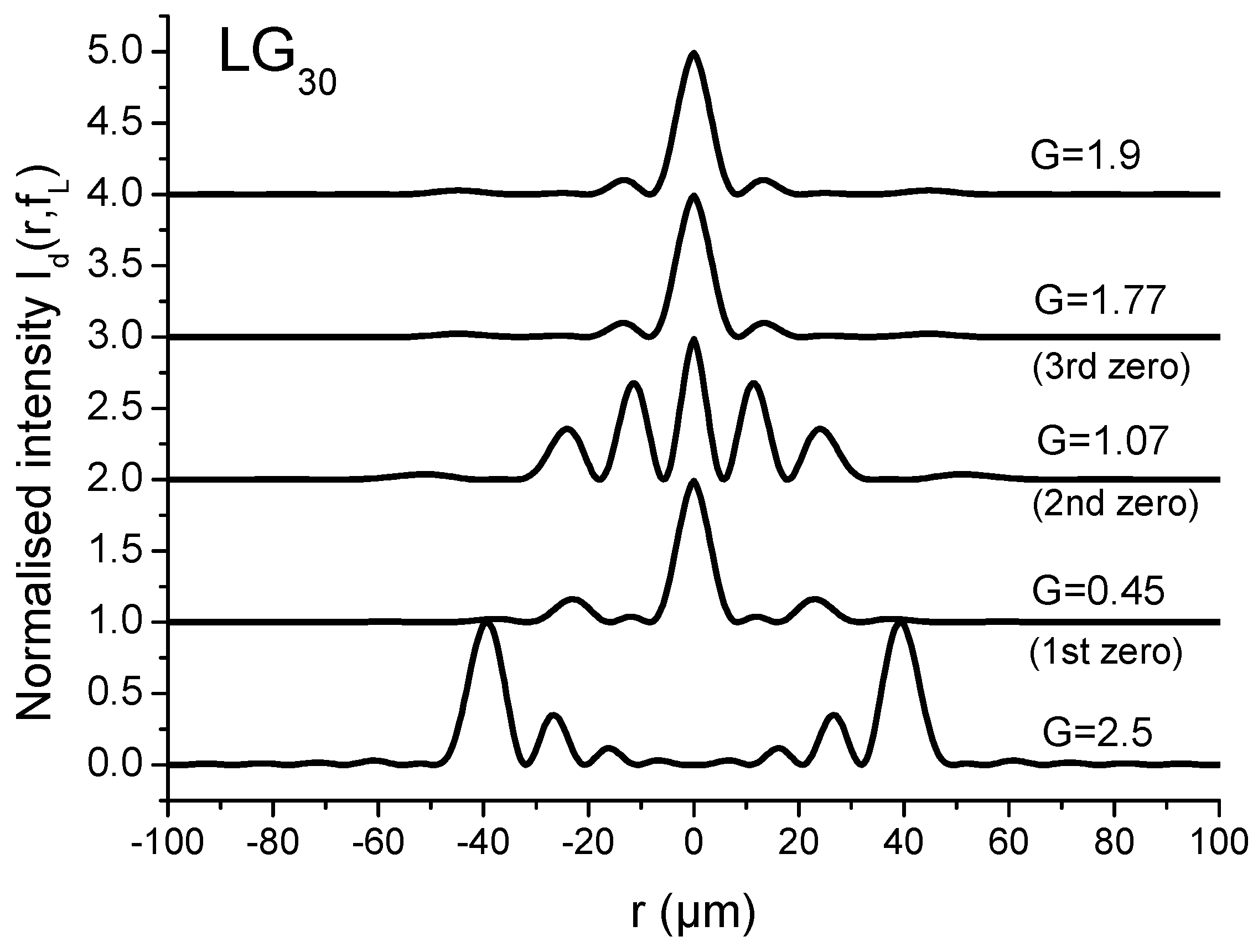
  • p = 3 → max1 → G = 0.45 (1st zero)
  • min > 0 → G = 1.06 (2nd zero)
  • max2 → G = 1.77 (3rd zero)
  • zero → G = 2.5
Table 2. Roots of Laguerre polynomials: L p ( ρ / W ) = 0 .
pValues of Ratio ρ/W for the Zeros
of Intensity of LGp0 Mode
10.707106
20.5411951.306562
30.4559461.0710461.773407
The interpretation of the zeros of on-axis intensity that are shown in Figure 9 is based on the value of the ratio η + defined as
η + = P + P t o t
where P + represents the optical power carried by the positive part of τ C ( ρ ) × E i n ( ρ ) , and P t o t is the total power of the L G p 0 beam. It has been shown [30] that the on-axis intensity distribution I d ( 0 , z = f L ) is an optical bottle beam when η + is in the range 67% to 74%.
It remains to be seen that depending upon the particular values of parameter G given above, the on-axis intensity profile is an OBB or a single-lobed beam profile. So as not to make the discussion too lengthy, we will focus on the L G 30 case for the four values of parameter G: 0.45; 1.06; 1.77; 2.5. The results are shown in Figure 10.
For the sake of completeness, it is necessary to examine the longitudinal distribution of the on-axis intensity for the different values of parameter G used in Figure 9. The results are shown in Figure 11, and effectively it is confirmed that for G = 2.5 we achieve an OBB centred on plane z = f L , and a main axial peak surrounded by bounces for the other values of G.
Having set out the different range of values for the CPP radius, the next step is to verify if the CPP is able to improve the tweezers’ performances by calculating the variations in Z L versus the CPP radius. The results are shown in Figure 12, and the following should be recognised:
(i)
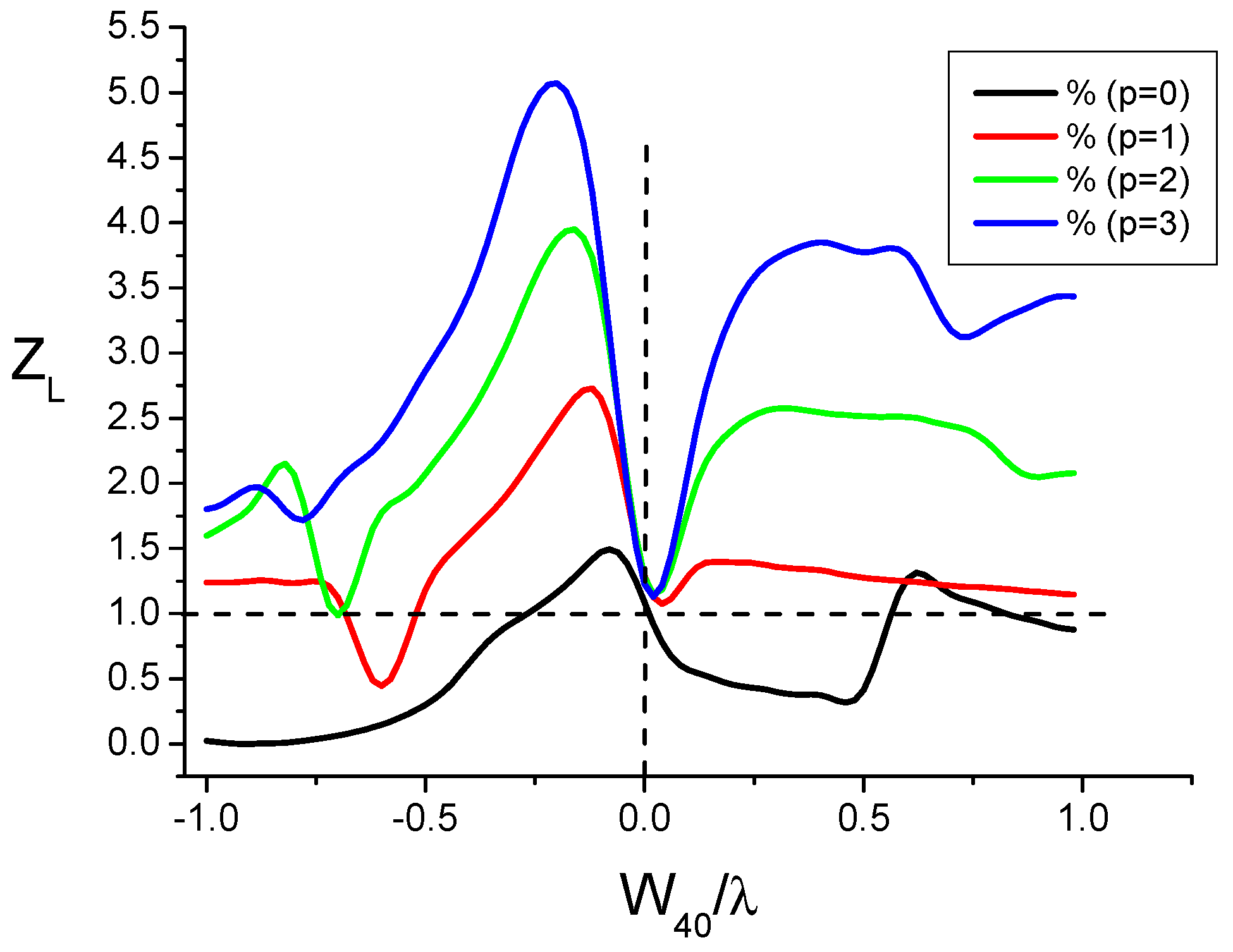
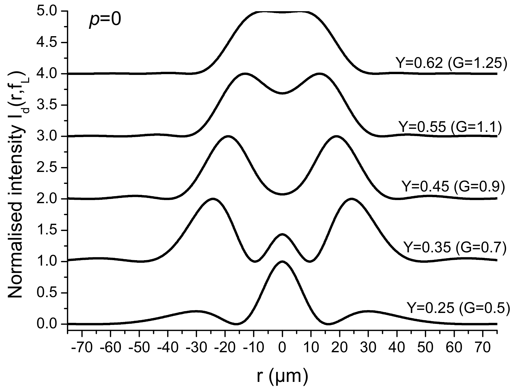
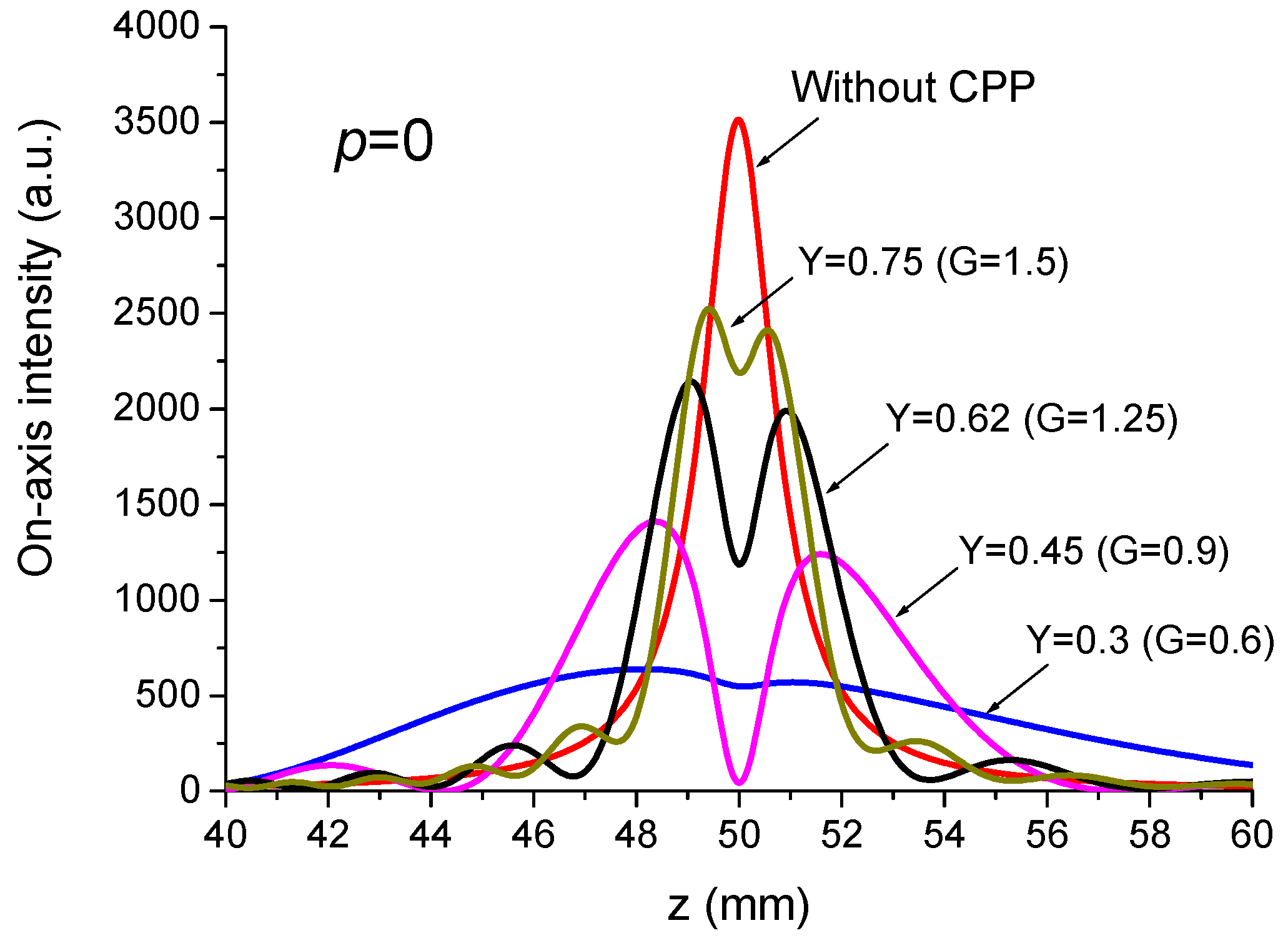
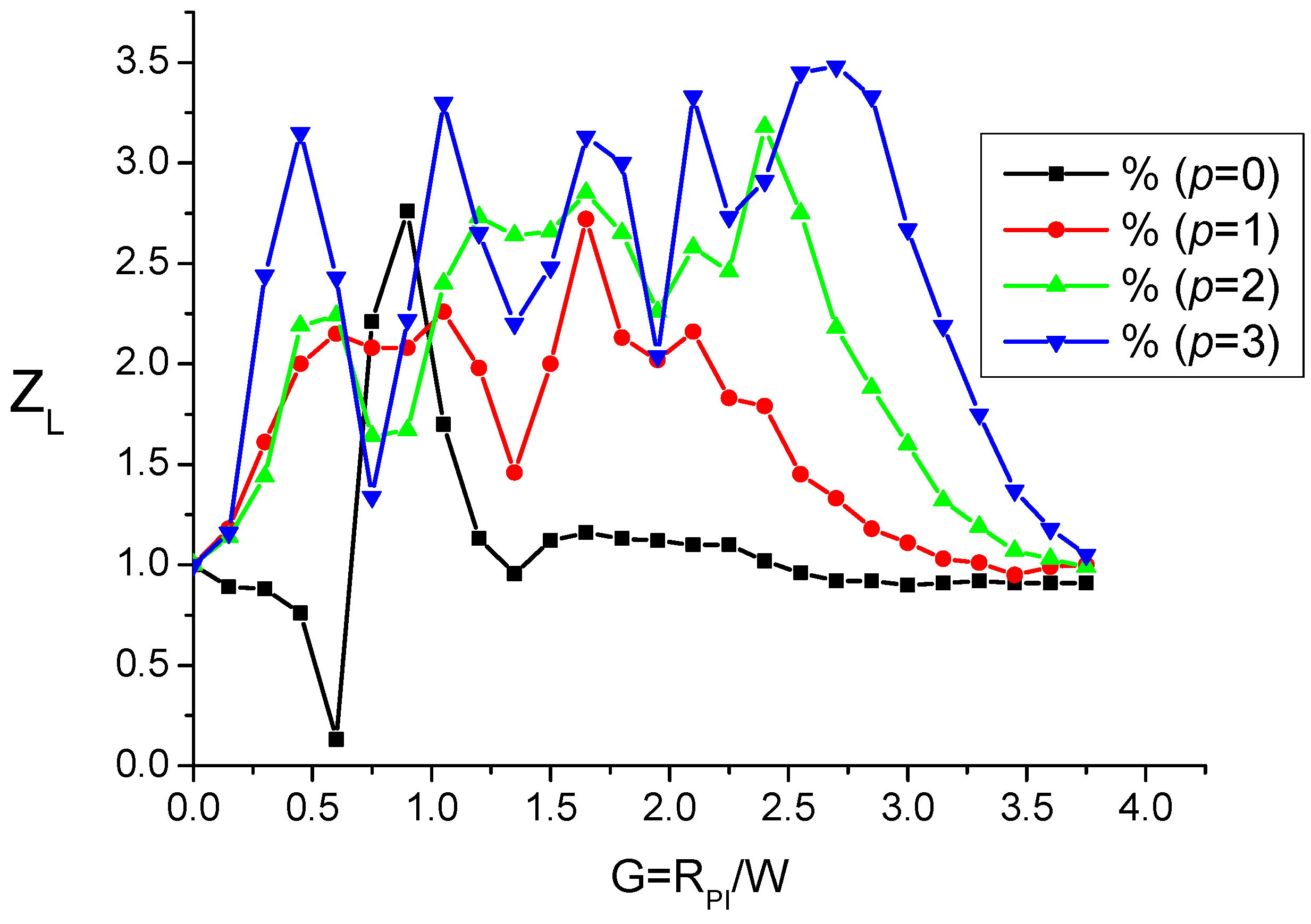
For p = 0, it is seen that the performance of the tweezers is reduced since Z L < 1 while it is boosted to about 2.5 for G = 0.9 , for which the focused Gaussian beam is an optical bottle beam, as seen above, well adapted for trapping particles with lower refractive indexes than the surrounding medium.
(ii)
For p 1 , it is seen that Z L can reach a value in the range of 2.5 to 3.2 for particular values of ratio G = R P I / W . By taking into account the plots in Figure 9, the improved values of Z L can correspond to the situation of a single-lobed beam or of an OBB depending on the value of ratio G = R P I / W . Consequently, it is necessary to envisage a possible adjusting of parameter G. This cannot be reasonably achieved by varying R P I because the device is obtained from the etching of a piece of glass. Reasonably, we have to envisage the variation in parameter W for adjusting the value of the ratio G = R P I / W for a given CPP as shown in Figure 13. Note that, by a simple longitudinal displacement, the CPP could allow to move from single-lobed-tweezers to OBB-tweezers while keeping, for instance, a Gaussian illumination.
Unlike the case of the incident laser beam subject to a pure spherical aberration giving rise to a focal shift shown in Figure 4, it is observed that the position of the best focus moves very little when parameter G = R P I / W is varied. This means that the CPP should not in any case be treated as a pure spherical aberration but rather as a mixing of different high-order spherical aberrations much more difficult to foresee the resulting effects. However, the original intention of this paper was the use of a CPP as a complex mixing of different orders of spherical aberrations for obtaining an improvement in the longitudinal figure of merit Z L as what was observed with a pure primary spherical aberration [3] and summarised in Figure 2. Given the results shown in Figure 12, one might conclude that the circular π-plate (CPP) giving rise to a discontinuous phase profile φ ( ρ ) is able to improve the longitudinal stability of the optical trap shown in Figure 1 and Figure 13. The value of Z L , which is of about 2.2 to 3.2, is a significant improvement compared to recent results obtained by L G p 0 rectification [4], spherical aberration [3] and nonlinear focusing [5,6]. During the last several years, the researchers took the challenge to operate the optical tweezers with non-Gaussian beams or more precisely with structured laser light [31,32,33,34,35,36,37,38]. The use of high-order radial Laguerre–Gauss modes has many advantages as discussed recently [31], but the majority of commercial lasers deliver a Gaussian beam. Consequently, the improvement in optical tweezers by using high-order modes requires the implementation of a homemade laser with an efficient control of the oscillating transverse mode [39,40,41,42,43,44,45].

4. Conclusions

The simplest optical tweezers are designed mainly by focusing a Gaussian laser beam. The trapping of a dielectric particle of nanometric size in the Rayleigh regime involves two longitudinal forces: a gradient force Fgrad proportional to the longitudinal gradient of the on-axis intensity, and a scattering force Fscat proportional to the longitudinal intensity distribution. The longitudinal stability (LS) of the trap depends on the ratio Fgrad/Fscat which increases when the focused beam waist size is reduced. This can be achieved by reducing the focal length f L of the focusing device which is in general a microscope objective. However, the focal length f L cannot obviously be reduced indefinitely, and consequently improving the tweezers efficiency requires an alternative strategy. One can quote, without wanting to be exhaustive, three techniques recently proposed. The first one is based on the use of a rectified high-order radial L G p 0 Laguerre–Gaussian beam instead of the usual Gaussian beam for illuminating the optical tweezers [4]. The second one involves the use of a complementary nonlinear-focusing based on the Kerr effect taking place in a thin layer of organic dye [5,6]. The third one involves a structuring of the incident L G p 0 beam by a pure primary spherical aberration [3].
In the present paper, the improvement in the tweezers’ longitudinal stability is based on the production of a steeper gradient of the longitudinal intensity distribution near the best focus point. This is achieved by setting on the path of the incident L G p 0 beam a particular phase aberration profile (PAP) allowing to increase the ratio Fgrad/Fscat, and consequently to improve the longitudinal stability of the trap without changing the focal length of the focusing device nor the incident beam power. We have proposed for realising the PAP the use of a simple binary diffractive optical element referred to as circular π-plate (CPP) able to generate positive or negative spherical aberrations [20] depending on its diameter. The longitudinal stability of tweezers illuminated by L G p 0 beams ( p 1 ) is multiplied by a factor varying from 2.2 to 3.2, provided that the incident beam passes through a circular π-plate (CPP) having the adequate size. When the incident beam is a Gaussian beam (p = 0) the longitudinal stability is multiplied by a factor equal to 2.7, but in this case, we are dealing with an OBB trap. It is found that the “single-lobbed-trap” regime is not improved by the presence of the CPP for p = 0.

Author Contributions

Investigation, A.H.; writing—original draft, K.A.-A. All authors have read and agreed to the published version of the manuscript.

Funding

This research received no external funding.

Institutional Review Board Statement

Not applicable.

Informed Consent Statement

Not applicable.

Data Availability Statement

Data are contained within the article.

Conflicts of Interest

The authors declare no conflicts of interest.

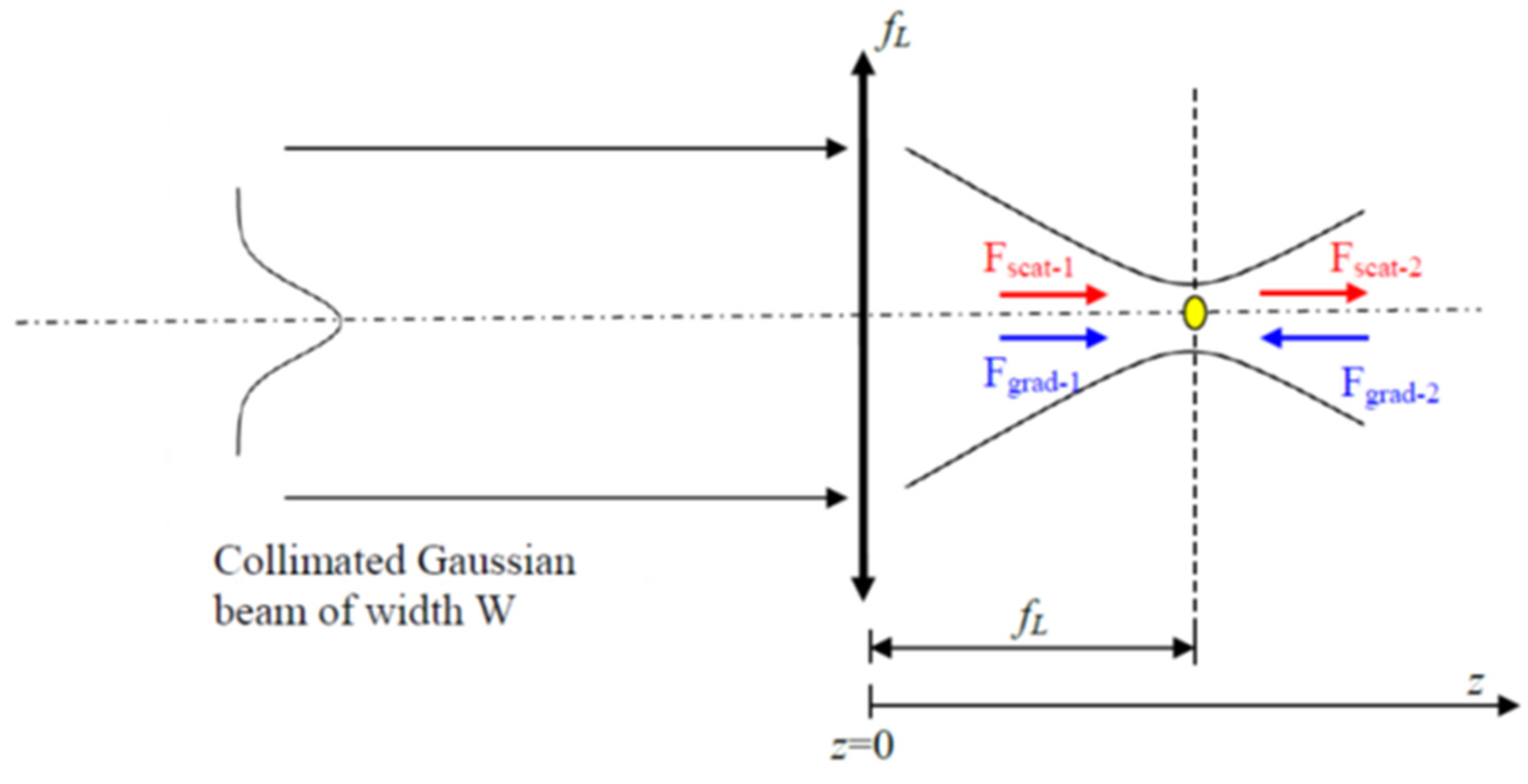
Appendix A. The Basics of Optical Tweezers

Optical tweezers are today an indispensable tool for manipulating non-invasively small particles. The initial work on the subject began in the 1970s by the pioneer Arthur Ashkin and remains a major challenge of intensive research. In this paper we consider the trapping of a spherical dielectric particle of radius a much smaller than the laser wavelength ( a < < λ ). In this context, the trapped particle is treated as a point-induced electric dipole interacting with the electromagnetic field associated with the focused laser beam. The theory of optical tweezers is described in detail in [8,9,10,11,12,13], and the essential elements are briefly recalled below. The experimental setup allowing the implementation of usual optical tweezers involves a Gaussian laser beam and a focusing lens as shown in Figure A1.
Figure A1. Optical trap set-up showing the scattering and gradient longitudinal forces. The focusing lens has a focal length fL. The yellow sphere represents the trapped particle.
Photonics 11 00744 g0a1
The trapping of the small dielectric particle involves two longitudinal forces as shown in Figure A1. The first one is a gradient force F g r a d proportional to the longitudinal gradient of the distribution of intensity. The second one is the scattering force F s c a t proportional to the longitudinal distribution of intensity. These two forces are given by
F g r a d = 4 π a 3 c m 2 1 m 2 + 2 z I d ( r , z )
F s c a t = 128 π 5 n m a 6 3 c λ 4 m 2 1 m 2 + 2 2 I d ( r , z ) z ^
where m = n p / n m is the ratio of the refractive index of the particle n p and the surrounding medium n m . The quantity I d ( r , z ) is the intensity distribution beyond the focusing lens, where r is the radial coordinate in plane z. In Equation (A1), the gradient ( ) operator has longitudinal and radial components giving rise to a longitudinal gradient force and a radial gradient force. Note that in Figure A1 the two forces are noted ( F g r a d 1 and F s c a t 1 ) in the region z < f L , and noted ( F g r a d 2 and F s c a t 2 ) in the region z > f L . In the next study, we will focus exclusively on the longitudinal components (r = 0) of the two forces F s c a t and F g r a d . When the incident laser beam is Gaussian, the on-axis intensity distribution I d ( 0 , z ) is symmetric with respect to the plane z = f L . Consequently, in this case we have F s c a t 1 = F s c a t 2 and F g r a d 2 = F g r a d 1 .
As shown in Figure A1, beyond the focal plane z = f L the scattering force pushes the particle along the direction z ^ of propagation of the laser beam while the gradient force pushes in the opposite direction. The condition that must be met in order to trap the particle is to fulfil the inequality F g r a d 2 > F s c a t 2 , where F g r a d ( F s c a t ) is the projection of F g r a d ( F s c a t ) on the z ^ direction. The ratio F g r a d / F s c a t expresses as follows
F g r a d F s c a t = K z ^ z I d ( r , z ) I d ( r , z )
With   K = 3 λ 4 32 π 4 n m a 3 m 2 + 2 m 2 1
The objective is to set a phase aberration profile (PAP) on the path of the incident beam (Figure 1) allowing to achieve a restructuring of the laser beam for improving the performances of the trap, i.e., increasing the ratio F g r a d / F s c a t for a given optical power. For that, we define dimensionless factors characterising the longitudinal forces improvement. For convenience, in the next we will express the stability of the optical trap by a relevant quantity noted R which is proportional to the ratio of the backward axial gradient and the forward scattering forces [4]
R = K z ^ . z I d ( 0 , z ) min I d ( 0 , z min )
z min is the longitudinal position where the ratio F g r a d / ( K F s c a t ) is minimum, as shown in Figure A2 for the case of a pure Gaussian beam. The position z min has to be viewed as a turning point where the gradient force can overcome the scattering force giving rise to an equilibrium for the trapped particle. For a Gaussian illuminating, the axial position z min is given by [46]
z min = z R / 3
where z R = ( π W 0 2 / λ ) = ( λ f L 2 ) / ( π W 2 ) is the Rayleigh distance of the focused Gaussian beam; W 0 is the beam-waist size of the focused beam.
Figure A2. Longitudinal variations in the normalised ratio F g r a d / ( K F s c a t ) .
Photonics 11 00744 g0a2
Parameter R represents a kind of stability efficiency whose value is important for the operation of the optical trap and can be controlled by the geometry of the laser beam focusing. This point is relevant but is not central in our study since we are rather interested to improve the value of parameter R thanks to the presence of a phase aberration profile (PAP) set on the path of the incident laser beam. In order to have a simple indicator allowing to estimate if the PAP presence (with PAP) improves or does not improves the trap stability compared to the case without the PAP (without PAP), it is convenient to have recourse to a dimensionless quantity noted Z L and defined as follows:
Z L = R with   PAP R without   PAP
The longitudinal stability of the trap is observed when the gradient force overcomes the scattering force, thus bringing back the particle pushed by the scattering force, so that the particle is trapped. The longitudinal stability of the trap is enhanced (reduced) if the dimensionless factor Z L is greater (smaller) than unity.

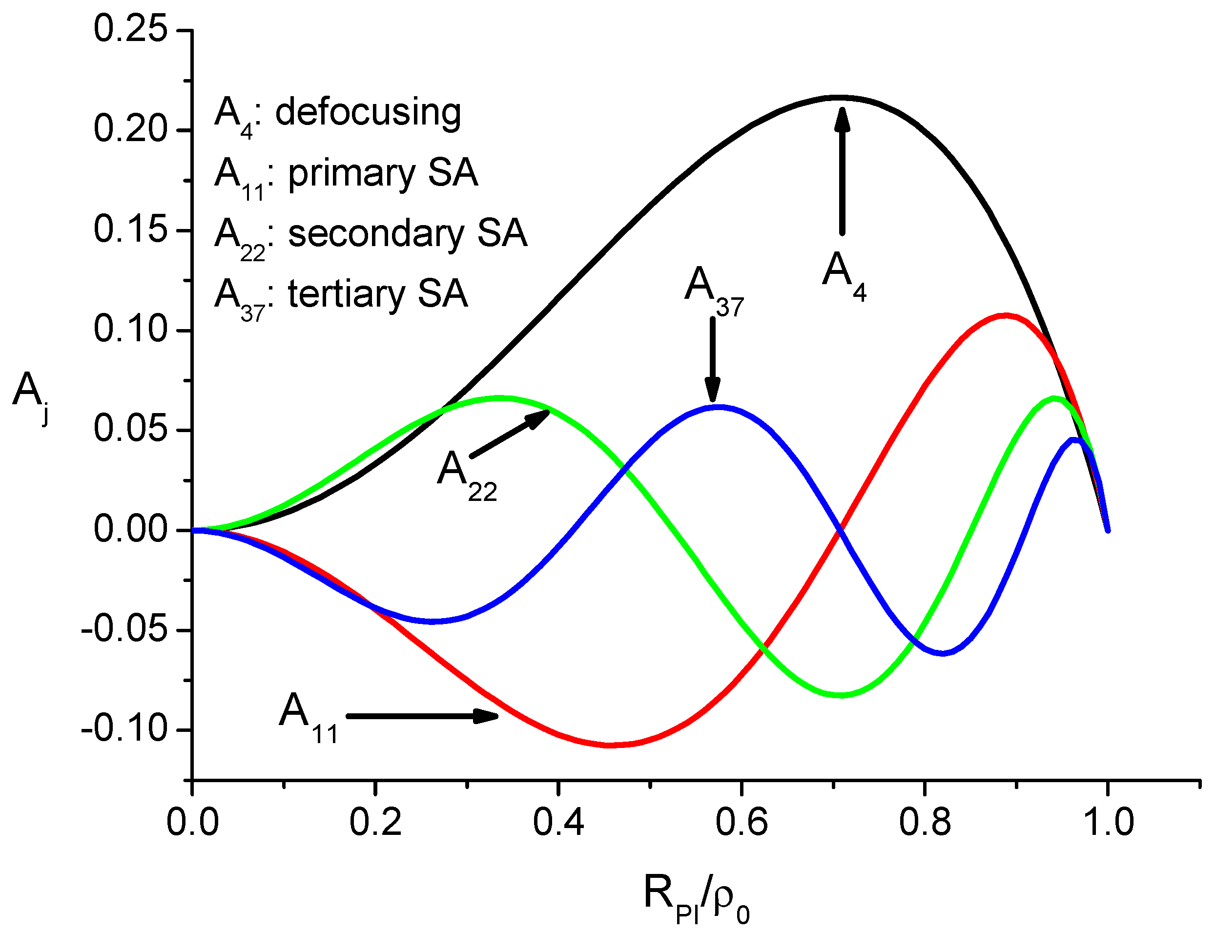
Appendix B. The Aberration Coefficients of the Circular Phase Plate

The incident collimated L G p 0 beam passing through the circular phase plate (CPP) defined by Equation (8) will have its wavefront distorted and will show a phase discontinuity. Consequently, since the wavefront is degraded, one can conclude that the CPP induces optical aberration which can be determined in the framework of Zernike polynomials [20]. It may be useful to recall here succinctly the main lines of the aberration coefficients determination. Before proceeding, strictly speaking, the aberrations coefficients should depend on the intensity profile of the incident L G p 0 , as shown in [24], making the findings difficult to interpret. We instead preferred to describe the incident beam in terms of plane waves limited by a circular pupil of radius ρ 0 given by Table 1. This incident plane wave has a spatial phase term (after the CPP) given by exp [ i k S ( ρ ¯ ) ] , where ρ is the radial coordinate, and ρ ¯ = ρ / ρ 0 . Following the lines of [24], the wavefront aberration function (WAF) S ( ρ ¯ ) is expanded as a linear combination of Zernike polynomials, Z j , as follows:
S ( ρ ¯ ) = 1 a j Z j ( ρ ¯ )
where the index j is a polynomial-ordering number, and a j are the expansion or aberration coefficients. Table A1 gives the Zernike polynomials (ZP) [19].
Table A1. Zernike polynomials allowing to calculate the aberration coefficients a 1 , a 4 , a 11 , a 22 and a 37 .
J Z j Type of aberration
4 3 ( 2 ρ ¯ 2 1 ) Defocus
11 5 ( 6 ρ ¯ 4 6 ρ ¯ 2 + 1 ) Primary spherical
22 7 ( 20 ρ ¯ 6 30 ρ ¯ 4 + 12 ρ ¯ 2 1 ) Secondary spherical
37 3 ( 70 ρ ¯ 8 140 ρ ¯ 6 + 90 ρ ¯ 4 20 ρ ¯ 2 + 1 ) Tertiary spherical
Taking into account Equation (8) defining the CPP, Figure A3 gives the radial variations in the WAF.
Figure A3. Transverse profile of the wave front aberration function of the wave passing through the circular phase plate.
Photonics 11 00744 g0a3
The aberration coefficients a j are given by the integral which can be found in [20,25]:
a j = 2 0 1 S ( ρ ¯ ) Z j ( ρ ¯ ) ρ ¯ d ρ ¯
For convenience, we use the dimensionless coefficients A j = a j / λ . By taking into account the variations in the WFA given in Figure A3, we finally obtain the normalised aberration coefficients as follows:
A j = 1 2 π 0 R ¯ P I Z j ( ρ ¯ ) ρ ¯ d ρ ¯
The variations in coefficients A j versus the normalised CPP radius R ¯ P I = R P I / ρ 0 are shown in Figure A4.
Figure A4. Variations in the normalised aberration coefficients A j of a circular π–plate (CPP) versus R P I , its radius. Note that ρ 0 is the radius of the unit circle (see Table 1) which depends on p, the mode order of the L G p 0 incident beam. Note that the plots are unchanged when the mode order p is changed.
Photonics 11 00744 g0a4

References

  1. Yoshida, A.; Asakura, T. Propagation and focusing of Gaussian laser beams beyond conventional diffraction limit. Opt. Commun. 1996, 123, 694–704. [Google Scholar] [CrossRef]
  2. Pu, J.; Zhang, H. Intensity distribution of Gaussian beams focused by a lens with spherical aberration. Opt. Commun. 1998, 151, 331–338. [Google Scholar] [CrossRef]
  3. Ait-Ameur, K.; Hasnaoui, A. Improving the longitudinal and radial forces of optical tweezers: A numerical study. Opt. Commun. 2024, 551, 130033. [Google Scholar] [CrossRef]
  4. Haddadi, S.; Ait-Ameur, K. Improvement of optical trapping effect by structuring the illuminating laser beam. Optik 2022, 25, 168439. [Google Scholar] [CrossRef]
  5. Quang, Q.H.; Doan, T.T.; Thanh, V.D.; Xuan, K.B.; Nguyen, L.L.; Manh, T.N. Nonlinear microscope objective using thin layer of organic dye for optical tweezers. Eur. Phys. J. D 2020, 74, 52. [Google Scholar] [CrossRef]
  6. Haddadi, S.; Ait-Ameur, K. Optical tweezers based on nonlinear focusing. Appl. Phys. B 2023, 129, 38. [Google Scholar] [CrossRef]
  7. Chai, H.S.; Wang, L.G. Improvement of optical trapping effect by using the focused high-order Laguerre-Gaussian beams. Micron 2012, 43, 887–892. [Google Scholar] [CrossRef] [PubMed]
  8. Neuman, K.; Block, S. Optical trapping. Rev. Sci. Instrum. 2004, 75, 2787–2809. [Google Scholar] [CrossRef] [PubMed]
  9. Ashkin, A. Acceleration and trapping of particles by radiation pressure. Phys. Rev. Lett. 1970, 24, 156–159. [Google Scholar] [CrossRef]
  10. Ashkin, A.; Dziedzic, J.M. Optical levitation by radiation pressure. Appl. Phys. Lett. 1971, 19, 282–285. [Google Scholar] [CrossRef]
  11. Harada, Y.; Asakura, T. Radiation forces on a dielectric sphere in the Rayleigh scattering regime. Opt. Commun. 1996, 124, 529–541. [Google Scholar] [CrossRef]
  12. Lang, M.J.; Block, S.M. Resource letter: LBOT-1: Laser-based optical tweezers. Am. J. Phys. 2003, 71, 201–215. [Google Scholar] [CrossRef]
  13. Dienerowitz, M.; Mazilu, M.; Dholakia, K. Optical manipulation of nanoparticles: A review. J. Nanophotonics 2008, 2, 021875. [Google Scholar] [CrossRef]
  14. Ota, T.; Sugiura, T.; Kawata, S.; Booth, M.J.; Neil, M.A.; Juskaitis, R.; Wilson, T. Enhancement of laser trapping force by spherical aberration correction using a deformable mirror. Jpn. J. Appl. Phys. 2003, 42, L701–L703. [Google Scholar] [CrossRef]
  15. Escobar, I.; Saavedra, G.; Martinez-Corral, M.; Lancis, J. Reduction of the spherical aberration effect in high-numerical-aperture optical scanning instruments. JOSA A 2006, 23, 3150–3155. [Google Scholar] [CrossRef]
  16. Nader, S.; Reihani, S.; Oddershede, L.B. Optimising immersion media refractive index improves optical trapping by compensating spherical aberrations. Opt. Lett. 2007, 32, 1998–2000. [Google Scholar]
  17. Zhong, M.C.; Wang, Z.Q.; Li, Y.M. Aberration compensation for optical trapping of cells within living mice. Appl. Opt. 2017, 56, 1972–1976. [Google Scholar] [CrossRef] [PubMed]
  18. Snyder, K.; Grier, D.G. Aberration compensation for enhanced holographic particle characterization. Opt. Express 2023, 31, 35200–35207. [Google Scholar] [CrossRef]
  19. Mafusire, C.; Forbes, A. Mean focal length of an aberrated lens. JOSA A 2011, 28, 1403–1409. [Google Scholar] [CrossRef]
  20. Bouzid, O.; Haddadi, S.; Fromager, M.; Cagniot, E.; Ferria, K.; Forbes, A.; Ait-Ameur, K. Focusing anomalies with binary diffractive optical elements. Appl. Opt. 2017, 56, 9735–9741. [Google Scholar] [CrossRef]
  21. Itoh, H.; Matsumoto, N.; Inoue, T. Spherical aberration correction suitable for a wavefront controller. Opt. Express 2009, 17, 14367–14373. [Google Scholar] [CrossRef]
  22. Theofanidou, E.; Wilson, L.; Hossack, W.J.; Arlt, J. Spherical aberration correction for optical tweezers. Opt. Commun. 2004, 236, 145–150. [Google Scholar] [CrossRef]
  23. Siegman, A.E. Analysis of laser beam quality degradation caused by quartic phase aberrations. Appl. Opt. 1993, 32, 5893–5901. [Google Scholar] [CrossRef]
  24. Mahajan, V.N. Zernike-Gauss polynomials and optical aberrations of systems with Gaussian pupils. Appl. Opt. 1995, 34, 8057–8059. [Google Scholar] [CrossRef]
  25. Mahajan, V.N. Zernike circle polynomials and optical aberrations of system with circular pupils. Appl. Opt. 1994, 33, 8121–8123. [Google Scholar] [CrossRef]
  26. Bourouis, R.; Ait-Ameur, K.; Ladjouze, H. Optimization of the Gaussian beam flattening using a phase plate. J. Mod. Opt. 1997, 44, 1417–1427. [Google Scholar] [CrossRef]
  27. Chaloupka, J.; Meyerhofer, D. Characterization of a tunable, single-beam ponderative-optical trap. JOSA B 2000, 17, 713–722. [Google Scholar] [CrossRef]
  28. Gahagan, K.T.; Swartzlander, G.A. Trapping of low-index microparticles in an optical vortex. JOSA B 1998, 15, 524–534. [Google Scholar] [CrossRef]
  29. Haddadi, S.; Fromager, M.; Louhibi, D.; Hasnaoui, A.; Harfouche, A.; Cagniot, E.; Ait-Ameur, K. Improving the intensity of a focused laser beam. In Proceedings of the SPIE LASE, Laser Resonators, Microresonators, and Beam Control XVII, San Francisco, CA, USA, 7–12 February 2015; Volume 9343, p. 93431R. [Google Scholar]
  30. Ait-Ameur, K. The advantages and disadvantages of using structured high-order but single Laguerre-Gauss LGp0 laser beams. Photonics 2024, 11, 217. [Google Scholar]
  31. Yang, Y.; Ren, Y.X.; Chen, M.; Arita, Y.; Rosales-Guzman, C. Optical trapping with structured light: A review. Adv. Photonics 2021, 3, 034001. [Google Scholar] [CrossRef]
  32. Forbes, A. Structured light from lasers. Las. Photon. Rev. 2019, 13, 1970043. [Google Scholar] [CrossRef]
  33. Forbes, A.; Oliveira, M.; Dennis, M.R. Structured Light. Nat. Photonics 2021, 15, 253–262. [Google Scholar] [CrossRef]
  34. Auyeung, R.C.Y.; Kim, H.; Mathews, S.; Piqué, A. Laser forward transfer using structured light. Opt. Express 2015, 23, 422–430. [Google Scholar] [CrossRef]
  35. Otte, E.; Denz, C. Optical trapping gets structure: Structured light for advanced optical manipulation. Appl. Phys. Rev. 2020, 7, 04108. [Google Scholar] [CrossRef]
  36. Häfner, T.; Strauβ, J.; Roider, C.; Heberle, J.; Schmidt, M. Tailored laser beam shaping for efficient and accurate microstructuring. Appl. Phys. A 2018, 124, 111. [Google Scholar] [CrossRef]
  37. Benstiti, A.; Bencheikh, A.; Ferria, K.; Chabou, S.; Boumeddine, O.C. Gaussian laser beam structuring using acousto-optic effect: A parametric characterization. Appl. Phys. B 2022, 128, 141. [Google Scholar] [CrossRef]
  38. Ando, T.; Ohtake, Y.; Matsumoto, N.; Inove, T.; Fukuchi, N. Mode purities of Laguerre-Gaussian beams generated via complex-amplitude modulation using phase-only spatial light modulators. Opt. Lett. 2009, 34, 34–36. [Google Scholar] [CrossRef] [PubMed]
  39. Huang, B.; Li, Q.; Yang, L.; Zhao, C.; Wen, S. Controlled higher-order transverse mode conversion from a fiber laser by polarization manipulation. J. Opt. 2018, 20, 024016. [Google Scholar] [CrossRef]
  40. Hu, A.; Lei, J.; Chen, P.; Wang, Y.; Li, S. Numerical investigation on the generation of high-order Laguerre-Gaussian beams in end-pumped solid-state lasers by introducing loss control. Appl. Opt. 2014, 53, 7845–7853. [Google Scholar] [CrossRef]
  41. Ishaaya, A.A.; Davidson, N.; Friesem, A.A. Very high-order pure Laguerre-Gaussian mode selection in a passive Q-switched Nd:YAG laser. Opt. Express 2005, 13, 4952–4962. [Google Scholar] [CrossRef]
  42. Huang, Y.J.; Chiang, P.Y.; Liang, H.C.; Su, K.W.; Chen, Y.F. High power Q-switched laser with high-order Laguerre-Gaussian modes: Application for extra-cavity harmonic generations. Appl. Phys. B 2011, 105, 385–390. [Google Scholar] [CrossRef]
  43. Dong, J.; Bai, S.C.; Liu, S.H.; Ueda, K.I.; Kaminskii, A.A. A high repetition rate passively Q-switched microchip laser for controllable transverse laser modes. J. Opt. 2016, 18, 055205. [Google Scholar] [CrossRef]
  44. Machavariani, G. Effect of phase imperfections on higher-mode selection with intracavity phase elements. Appl. Opt. 2004, 43, 6328–6333. [Google Scholar] [CrossRef] [PubMed]
  45. Senatsky, Y.; Bisson, J.-F.; Li, J.; Shirakawa, A. Laguerre-Gaussian modes selection in diode-pumped solid-state lasers. Opt. Rev. 2012, 19, 201–221. [Google Scholar] [CrossRef]
  46. Ashkin, A.; Dziedzic, J.M.; Bjorkholm, J.E.; Chu, S. Observation of a single-beam gradient force optical trap for dielectric particles. Opt. Lett. 1986, 11, 288–290. [Google Scholar] [CrossRef]
Figure 1. Optical trap set-up showing the focusing of a LGp0 beam restructured by a phase aberration profile φ ( ρ ) for trapping a particle taking the form of a green sphere.
Photonics 11 00744 g001
Figure 2. Variations in the figure of merit Z L versus W 40 / λ , the normalised primary spherical aberration coefficient. Z L > 1 ( Z L < 1 ) indicates that the longitudinal stability of the trap is improved (reduced).
Photonics 11 00744 g002
Figure 3. Distribution of the on-axis intensity of a L G 30 beam passing through a lens of focal length fL = 50 mm, and a primary spherical aberration characterised by the coefficient W 40 .
Photonics 11 00744 g003
Figure 4. Variations in the relative variations in z max ; the position of the best focus versus the normalised spherical aberration coefficient.
Photonics 11 00744 g004
Figure 5. Axial distribution of the longitudinal gradient of the on-axis intensity for a L G 30 beam passing through a lens of focal length fL = 50 mm, and a primary spherical aberration characterised by the coefficient W 40 .
Photonics 11 00744 g005
Figure 6. Variations in the relative variations in z min , the position where the gradient force can overcome the scattering force defining the turning point of the optical trap.
Photonics 11 00744 g006
Figure 7. Focused intensity distribution of a Gaussian beam diffracted through a circular π-plate having a normalised radius Y = R P I / ρ 0 or G = R P I / W .
Photonics 11 00744 g007
Figure 8. On-axis intensity of a Gaussian beam diffracted through a circular π-plate having a normalised radius Y = R P I / ρ 0 and focused by a lens of focal length fL = 50 mm.
Photonics 11 00744 g008
Figure 9. Variations in the on-axis intensity I d ( 0 , z = f L ) in the focal plane of the focusing lens versus the normalised radius of the circular π-plate.
Photonics 11 00744 g009
Figure 10. Focused intensity radial distribution in plane z = f L of a L G 30 beam diffracted through a circular π-plate having a normalised radius G = R P I / W .
Photonics 11 00744 g010
Figure 11. On-axis intensity of a L G 30 beam diffracted through a circular π-plate having a normalised radius Y = R P I / ρ 0 and focused by a lens of focal length fL = 50 mm. The case without CPP is indicated by G = INF.
Photonics 11 00744 g011
Figure 12. Variations in the longitudinal figure of merit Z L versus G = R P I / W , the normalised radius of the circular π-plate (CPP).
Photonics 11 00744 g012
Figure 13. Set-up allowing for adjusting the parameter G = R P I / W for a given circular π-plate.
Photonics 11 00744 g013
Table 1. Variations in ρ 0 of the radius of the unit circle with the mode order p of the incident LGp0 beam, where W is the width of the Gaussian term in Equation (3).
p0123
ρ 0 2 W2.55 W3 W3.35 W
Disclaimer/Publisher’s Note: The statements, opinions and data contained in all publications are solely those of the individual author(s) and contributor(s) and not of MDPI and/or the editor(s). MDPI and/or the editor(s) disclaim responsibility for any injury to people or property resulting from any ideas, methods, instructions or products referred to in the content.

