Time-of-Flight Camera Intensity Image Reconstruction Based on an Untrained Convolutional Neural Network

Abstract

With the continuous development of science and technology, laser ranging technology will become more efficient, convenient, and widespread, and it has been widely used in the fields of medicine, engineering, video games, and three-dimensional imaging. A time-of-flight (ToF) camera is a three-dimensional stereo imaging device with the advantages of small size, small measurement error, and strong anti-interference ability. However, compared to traditional sensors, ToF cameras typically exhibit lower resolution and signal-to-noise ratio due to inevitable noise from multipath interference and mixed pixels during usage. Additionally, in environments with scattering media, the information about objects gets scattered multiple times, making it challenging for ToF cameras to obtain effective object information. To address these issues, we propose a solution that combines ToF cameras with single-pixel imaging theory. Leveraging intensity information acquired by ToF cameras, we apply various reconstruction algorithms to reconstruct the object’s image. Under undersampling conditions, our reconstruction approach yields higher peak signal-to-noise ratio compared to the raw camera image, significantly improving the quality of the target object’s image. Furthermore, when ToF cameras fail in environments with scattering media, our proposed approach successfully reconstructs the object’s image when the camera is imaging through the scattering medium. This experimental demonstration effectively reduces the noise and direct ambient light generated by the ToF camera itself, while opening up the potential application of ToF cameras in challenging environments, such as scattering media or underwater.

1. Introduction

Three-dimensional (3D) imaging and multi-pixel range-finding constitute some of the most important and innovative fields in the science and engineering of image sensors in the past decades [1], where the time-of-flight (ToF) camera is one of most-used 3D imaging techniques, due to its characteristics of a miniaturized structure, low cost, and direct readout of depth images [2]. Though the principle of the ToF has been proposed by Galileo since the 17th century, the first generation of ToF cameras was invented after the important parameters for the cameras’ performance were precisely defined in the early 1990s [3]. With the development of various supporting techniques, many cost-efficient solutions to the ToF cameras have been implemented, and some limitations have been resolved in different imaging scenarios, such as transient imaging [4,5,6], multi-view stereo methods [7], calculation of the 3D motion speed of an object [8], and the transient capture of light [6,9]. In recent years, some new methods were proposed to acquire 3D images by combining the ToF methods with single-pixel imaging [10,11,12]. Generally, the ToF measurement techniques can be mainly classified in two categories, i.e., so-called direct-ToF (D-ToF) and indirect-ToF (I-ToF), according to the measurement methods of the round-trip time of optical signals [13,14], where both pulsed and continuous wave modulated light sources in each technique are most commonly used [15]. For example, Jeremias and Brockherde’s pioneering work on electronics-based sensors for 3D imaging is a pulsed I-ToF technique [16], while Buttgen’s group gave a solution for high-precision 3D imaging in real-time used a continuous wave modulated I-ToF technique [17]. Additionally, single photon avalanche diodes (SPADs) are detectors capable of capturing individual photons with very high time-of-arrival resolution, in the order of a few tens of picoseconds. By reason of their picoseconds timing resolution, SPADs have become a natural candidate for D-ToF techniques [18,19,20,21] since it was first proposed by Albota and Entwistle in 2002 [22]. Compared with the other 3D imaging methods, such as structured light 3D imaging [23,24,25,26,27] and the binocular vision 3D imaging [28], ToF cameras can acquire both the depth and intensity information of a scene in real time [29], which greatly enhance its application prospects. Therefore, several ToF cameras have been widely applied in both some commercial and research fields, such as multi-media, consumer electronics, security/surveillance [30], super-resolution imaging [31,32], non-line-of-sight imaging [33], and autonomous driving [34]. However, though great progress has been made for ToF cameras, the low pixel resolution and signal-to-noise ratio (SNR) in these applications are still bottlenecks that have not been broken through so far [35].

Computational ghost imaging (CGI), which was theoretically proposed by Sharpio [36] more than a decade ago, is based on ghost imaging (GI) modality [37,38], where only a detection beam actually exists and is captured by a single-pixel bucket detector in the detection plane, while the optical intensity distribution in the reference beam can be obtained by data processing. Therefore, a ghost image of a target object can be reconstructed by the intensity (fluctuation) correlation between the bucket and reference signals, just like a traditional GI does, which is even also available in harsh environments such as atmospheric turbulence [39] or scattering media [40], where traditional imaging methods do not work. Fortunately, given the success of the compressed sensing (CS) [31,41,42,43] algorithm in GI, CS is a naturally suitable algorithm for computational ghost image reconstructions for sparse targets, because CGI has the same core mechanics with GI [44,45,46,47,48,49,50,51]. Due to the sparsity and noise in the intensity and depth maps acquired by the ToF sensor, we choose to use CS algorithms to process these maps for their good denoising performance and high resolution at low sampling rates. Though CS provides an alternative choice for improving the performance of CGI by its various modified image reconstruction algorithms, its application is more or less limited by the assumption of strong sparsity and the reconstruction process [52,53,54]. The emergence of deep learning (DL) [33,55,56,57,58] provides an opportunity to eliminate the constraint of sparsity to recover the images by data trained and untrained strategies at an ultralow sampling rate (SR) [58,59,60,61,62]. Meanwhile, a variety of novel computational 3D imaging techniques, including those based on the ToF and SPI, all gave a promising potential applications in different imaging fields [12,63,64,65,66,67,68].

In this paper, in a single-pixel imaging (SPI) experiment based on structure detection, a ToF camera is used as a bucket detector, and different algorithms are used to reconstruct the likeness of the target object based on the intensity information from the ToF sensor, and compare it with the original image output from the ToF camera (ToF image). It is found that the scheme based on TVAL3 algorithm and untrained DL can obtain higher quality images at a very low sampling rate. In addition, we have experimented with ToF cameras by scattering media, and the SPI-based CS and DL methods can recover images clearly, while the normal ToF methods cannot. We believe that the ToF camera may be suitable for multi-noise and complex environments, such as scattering media or underwater in similar schemes.

2. Basic Theories and Principles

2.1. Ranging Principle of ToF Cameras

The time-of-flight camera is a 3D imaging technology that uses the time difference of light beam reflection from the surface of objects to measure distances. It has advantages over traditional cameras in terms of measuring object distances because it can perform measurements regardless of lighting conditions. The modulation of the light source in time-of-flight cameras can be categorized into pulse modulation and continuous wave (CW) modulation. Pulse modulation is a technique that converts analog signals into digital signals, while continuous wave modulation is a modulation technique that adjusts the amplitude, frequency, phase, and other characteristics of the carrier signal using the frequency of the modulation signal, thereby enabling the process of information transmission.

The schematic diagram in Figure 1 illustrates the working principle of CW modulation. When using the continuous wave measurement method, it is necessary to utilize phase demodulation to accurately calculate the flight time of photons in space. Phase demodulation involves the emission of modulated continuous wave signals by the illumination module. These signals reach the object being measured and reflect back to the receiving module. The receiving module utilizes a demodulation signal identical to the modulation signal from the light source to complete the demodulation process, thereby extracting the phase variations of the light signal. We use the most commonly used continuous sinusoidal wave modulation, as shown in Figure 1, to derive the measurement principle of the continuous wave modulation mode.

Let us assume that the emitted sinusoidal signal $s\left(t\right)$ can be represented by Equation (1),

$$\begin{array}{c}\hfill s\left(t\right)=a·(1+sin(2\pi ft\left)\right),\end{array}$$

(1)

In Equation (1), where a represents the amplitude of the transmitted signal and f is the frequency, after a time period $\Delta t$, the received signal has an amplitude of A. Taking into account that the majority of received photon signals are superimposed on the image, we need to introduce an offset value B to obtain the actual measurement value. $r\left(t\right)$ can be represented by Equation (2),

$$\begin{array}{c}\hfill \begin{array}{c}r\left(t\right)=A·(1+sin(2\pi f(t-\Delta t)\left)\right)+B,\hfill \\ =A·(1+sin(2\pi ft-\Delta \varphi \left)\right)+B.\hfill \end{array}\end{array}$$

(2)

In Figure 1, the four sampling time intervals are equal, all denoted as ${\displaystyle \frac{T}{4}}$. Let us assume that $t_1=0$, $t_2={\displaystyle \frac{T}{4}}$, $t_3={\displaystyle \frac{T}{2}}$, $t_4={\displaystyle \frac{3T}{4}}$. Based on these four sampling times, we can establish four sets of equations: $r_1$, $r_2$, $r_3$, and $r_4$. By performing calculations on these four sets of equations, we can determine the amplitude A and phase delay $\Delta \varphi$ of the received sinusoidal signal,

$$\begin{array}{c}\hfill \Delta \varphi =arctan\left({\displaystyle \frac{r_3-r_4}{r_1-r_2}}\right),\end{array}$$

(3)

$$\begin{array}{c}\hfill A={\displaystyle \frac{1}{2}}\sqrt{{\left(r_1-r_2\right)}^2+{\left(r_3-r_4\right)}^2}.\end{array}$$

(4)

Using the four integral time accumulated charges $S_1$, $S_2$, $S_3$ and $S_4$ to denote $\Delta \varphi$ and A,

$$\begin{array}{c}\hfill \Delta \varphi =arctan\left({\displaystyle \frac{S_3-S_4}{S_1-S_2}}\right),\end{array}$$

(5)

$$\begin{array}{c}\hfill A={\displaystyle \frac{1}{2}}\sqrt{{\left(S_1-S_2\right)}^2+{\left(S_3-S_4\right)}^2}.\end{array}$$

(6)

The offset B can be expressed as

$$\begin{array}{c}\hfill B={\displaystyle \frac{1}{4}}(S_1+S_2+S_3+S_4),\end{array}$$

(7)

Based on the calculated phase values $\Delta \varphi$, the distance information can be expressed in Equation (8),

$$\begin{array}{c}\hfill d={\displaystyle \frac{c}{4\pi f}}\Delta \varphi .\end{array}$$

(8)

The amplitude A and offset B of the modulated light in a ToF camera measurement system affects the accuracy of the measurement, and the values of A and B indirectly reflect the accuracy of the depth measurement, so the accuracy of the measurement can be approximated as Equation (9),

$$\begin{array}{c}\hfill {\sigma }_d={\displaystyle \frac{c}{4\sqrt{2}\pi f}}·{\displaystyle \frac{\sqrt{A+B}}{c_d·A}},\end{array}$$

(9)

Here, $c_d$ is the modulation contrast. It can be seen from the principle that the measurement accuracy of the time-of-flight camera does not change with the measurement distance, so the ToF depth camera is also more resistant to interference.

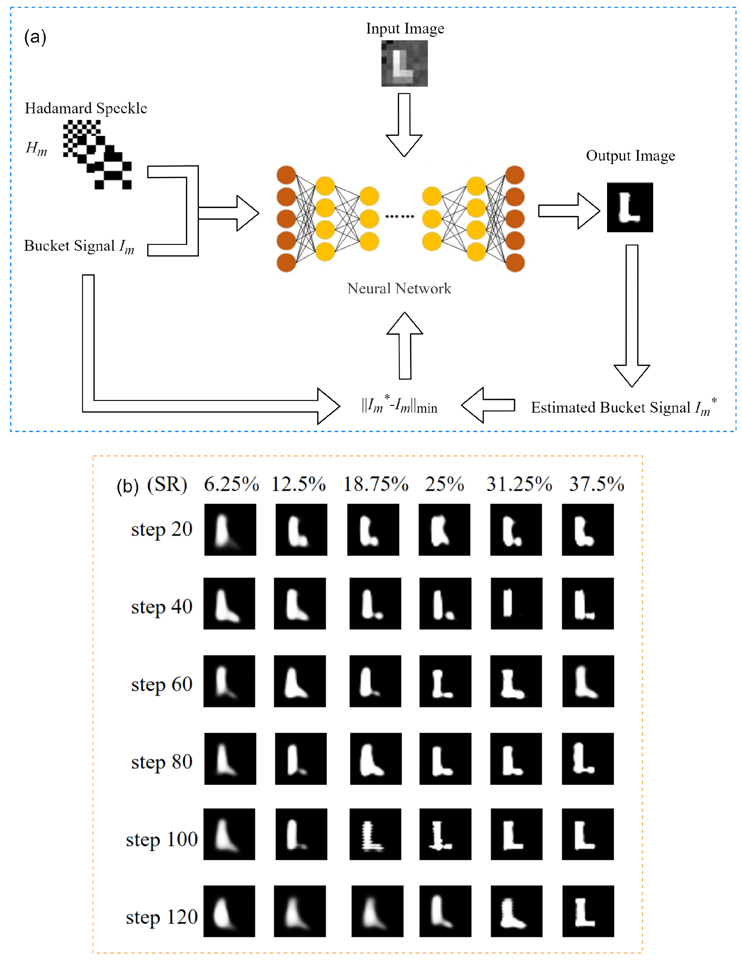
2.2. Untrained Neural Network Architecture

In the field of single-pixel imaging (SPI), correlation algorithms or compressed sensing (CS) algorithms are typically used to reconstruct images of target objects. However, traditional methods often struggle to achieve high-quality reconstruction at low sampling rates, and the numerous iterative operations significantly increase both imaging time and computational cost. Data-driven deep learning (DL) algorithms have shown promise in addressing these challenges. Unfortunately, issues such as the difficulty of obtaining sufficient training data, limited model generalization, and lengthy training times remain significant hurdles. To overcome these challenges, computational imaging schemes based on the concept of deep image prior (DIP) have been proposed. These schemes integrate the physical processes of SPI into untrained neural networks to generate images of target objects, offering notable advantages in terms of generalizability and interpretability. In this approach, only the detected one-dimensional barrel signals are fed into the neural network, which then outputs optimal reconstruction results. This process adheres to the strict constraints imposed by the interactions between the neural network and the physical processes of SPI during image reconstruction. The image reconstruction process can be represented by Equation (10),

$$\begin{array}{c}\hfill R_{\theta \ast }=arg\underset{\theta }{min}{∥P_i{R}_{\theta }\left(z\right)-y_i∥}^2,\end{array}$$

(10)

Here, $P_i$ is the modulation mask pattern, $y_i$ is the measured one-dimensional bucket signal, $\widehat{T}=R_{\theta }\left(z\right)$ is the output of the neural network, and ${∥P_i{R}_{\theta }\left(z\right)-y_i∥}^2$ denotes the error (loss function) between the actual measured and bucket signals estimated by the network. In addition, a physically enhanced DL framework for SPI is proposed to combine data-driven DL-based and physical model-driven untrained neural networks in order to further improve the generalization of the network to solve the computational imaging inverse problem.

Compared with traditional iterative algorithms, data-driven DL-based reconstruction methods have been proven to be effective in avoiding huge computational burden and obtaining high-quality reconstruction results. Unfortunately, however, it is usually difficult to obtain sufficient training data in many tasks, and the limited generalization ability of the model and the long time for model training become a lingering haze. Recently, untrained convolutional neural network schemes based on DIP have attracted great attention in computational imaging, which is able to make an appropriate compromise between image quality and computational cost. DIP states that by stopping the network optimization in advance, the neural network can use its structure to solve the imaging inverse problem without the need of a large amount of data used to train the neural network. This feature compensates for the shortcomings of existing data-driven DL.The reconstruction process of DIP can be expressed as the function shown in Equation (11),

$$\begin{array}{c}\hfill R_{\theta \ast }=arg\underset{\theta }{min}{∥R_{\theta }\left(z\right)-O^{\prime }∥}^2,\tilde{O}=R_{\theta \ast }\left(z\right),\end{array}$$

(11)

In Equation (11), $O^{\prime }$ is the degraded model of the target object, $\tilde{O}$ is the image recovered by the untrained neural network, and z is a fixed random vector, $arg\underset{\theta }{min}$ represents the process of solving the minimization problem. $R_{\theta }$ is a convolutional neural network defined by a set of weights and a bias parameter $\Theta$. Specifically, suppose that given a randomly initialized convolutional neural network, a function space is also defined. Assuming that the image of the object we are looking for is in this space, the process of reconstructing the image through the network is the process of updating the weights in the neural network and finding the appropriate parameter $\theta \ast \in \Theta$.

Inspired by the DIP and SPI approaches, we integrate the imaging physics model of ToF into a randomly initialized untrained convolutional neural network to obtain high-quality reconstructed images by interacting with the imaging physics process during network optimization, which allows for low time consumption in data preparation and image reconstruction. In our approach, the reconstruction formula of the target image can be represented by Equation (12),

$$\begin{array}{c}\hfill R_{\theta \ast }=arg\underset{\theta }{min}{∥H_j{R}_{\theta }\left(z\right)-{y^{\prime }}_j^t∥}^2+\xi T\left[R_{\theta }\left(z\right)\right].\end{array}$$

(12)

As we mentioned, the input z to the neural network can be a blurred image obtained using conventional reconstruction methods, and $H_j{R}_{\theta }\left(z\right)$ denotes the inner product between each modulation mask and the target object image. During the network iteration process, the network will find the appropriate parameter $\theta \ast$ to optimize its network structure. $\xi T\left[R_{\theta }\left(z\right)\right]$ is the TV regularization constraint that improves the quality of the reconstructed image, and $\xi$ is the intensity. In Equation (12), ${∥H_j{R}_{\theta }\left(z\right)-{y^{\prime }}_j^t∥}^2$ denotes the error between the experimentally measured bucket signals and the bucket signals estimated by the untrained neural network, which we use as the loss function of the network. According to Equation (12), the neural network weights are continuously updated during the iterative operation to minimize the error between the bucket signals. When the error is smaller, the estimated bucket signal is closer to the real bucket signal, and the network output is closer to the target object image.

The image reconstruction process of our proposed method is shown in Figure 2a, where the input image we use is the result of TVAL3 reconstruction. This is because the TVAL3 reconstructed image introduces the physical prior of the target object image, which will accelerate the convergence of the network. When the input image does not have physical prior information, the best reconstructed image can be obtained with the minimum number of iterations. Figure 2b shows the reconstructed image during iterations of the network for different sampling rates and learning rates.

3. Experimental Scheme and Analysis of Results

3.1. Introduction to the Experimental Setup and Experimental Principles

The SPI imaging scheme is shown in Figure 3, in which a target object illuminated by a light beam is imaged on a DMD, and then one of the light beams reflected from the DMD is captured by a barrel detector through a collection lens. As an indirect imaging method, the image can be retrieved by a correlation calculation between the modulation matrix and the actual captured single-pixel optical signal carrying information about the target object.

We assume that the pixelated target object image is $T(x,y)$, which contains a total of $N=x·y$ pixel points. In SPI, a series of modulation patterns $P_i(x,y)$ are usually loaded onto the DMD used to spatially modulate the beam carrying the object information, where $i=1,2,...,N$ represents the number of modulation patterns. The DMD-modulated one-dimensional light intensity signal collected by the barrel detector can be denoted as $y_i$, which corresponds to the result of the object image being modulated by a certain pair of scattering patterns, a process that can be mathematically represented as

$$\begin{array}{c}\hfill y_i=\underset{x}{\int }\underset{y}{\int }{P}_i(x,y)·T(x,y)dxdy,\end{array}$$

(13)

The barrel signal for all submeasurements can be expressed as

$$\begin{array}{c}\hfill S=PT.\end{array}$$

(14)

We can use the known modulation pattern P and the detected barrel signal S to solve for the image of the target object. The signal can be expressed in terms of normalized intensity correlation as

$$\begin{array}{c}\hfill {\mathrm{g}}^{\left(2\right)}(x,y)={\displaystyle \frac{(1/N){\displaystyle \sum _{i=1}^N}{S}_i{P}_i(x,y)}{(1/N){\displaystyle \sum _{i=1}^N}{S}_i(1/N){\displaystyle \sum _{i=1}^N}{P}_i(x,y)}},\end{array}$$

(15)

Here, S is the ith($i=1,2,\cdots ,N$) single-pixel signal, $P_i(x,y)$ is the ith modulation scatter, and x and y are the row pixel coordinates and column pixel coordinates of each modulation base of the DMD.

It is well known that ToF cameras can simultaneously output intensity and depth data carrying information about the target object, both of which are derived from the number of photons received by the ToF sensor in a certain period of time. Their difference is that the intensity information can be obtained as directly as by using a detector, while the depth map is obtained by calculating the phase difference of different phase signals through a complex mathematical operation in Equation (8). However, they are essentially determined by the statistics of the number of photons. Therefore, when the ToF camera is used as a barrel detector, both intensity information and depth information can be used in the SPI system of Figure 3. That is, by replacing the barrel signal intensity information with depth information, Equation (15) still holds, and we have published this result in [69].

In order to verify the feasibility of the proposed scheme, based on the experimental setup in Figure 3, a ToF camera was used for the SPI experiments; we used a 320 × 240 pixel ToF camera (OPT8241, Texas Instruments, Dallas, TX, USA) instead of a barrel detector, and inserted a total reflective prism (TRP) between the DMD and the detector to regulate the optical path, and the rest of the experimental setup was similar to that of the conventional SPI in Figure 3. In Figure 4, a flat object with an infrared light source at a wavelength of 850 nm is imaged with an imaging lens with a focal length of 50 mm on the surface of the optical unit of a DMD (DLP LightCrafter 4500, Texas Instruments), in which an all-reflecting prism is inserted in the optical path to accommodate the adjustment of the detection system. One of the DMD reflected beams carrying the coded pattern information is captured by a ToF sensor, which is designed to be synchronized with the light source of the ToF camera. The intensity information and depth information output from the ToF camera are calculated inside the camera.

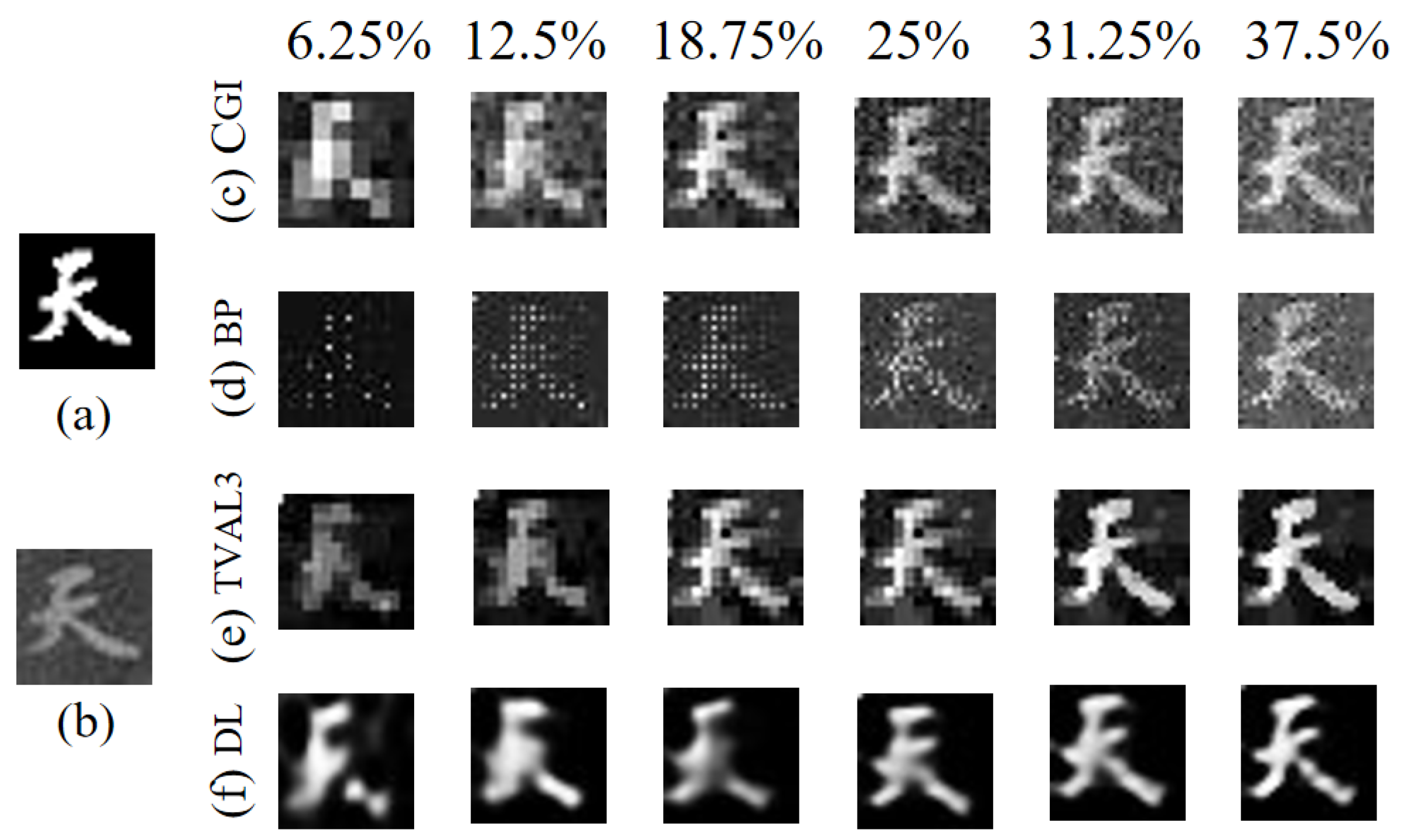
3.2. Experimental Results and Cause Analysis

Our experiments are conducted under indoor conditions with ambient light to recover the target object to be measured, using the scheme shown in Figure 4 for the acquired ToF intensity information. The reconstructed target shown in Figure 5a is an object with a pixel value of 32 × 32 size. In order to highlight the superiority of our proposed method, Figure 5b shows the ToF intensity map obtained directly with the utilized ToF camera, which has a noticeable background noise and lower contrast compared to the original image in Figure 5a. In our experiments, whichever algorithm is used, the bucket signal is obtained by summing the intensities of all pixels in the region of interest of the ToF sensor and synchronizing them with the Hadamard base projected onto the DMD. Four commonly used image reconstruction algorithms are selected including CGl algorithm, Base Tracking (BP) algorithm, Total Variation Augmented Lagrangian Alternating Direction (TVAL3) algorithm and DL algorithm for recovering the images in the following experiments. As shown in Figure 5, the images are reconstructed at sampling rates of 6.25%, 12.5%, 18.75%, 25%, 31.25% and 37.5%.

In Figure 5, When the sampling rate is 6.25%, BP reconstructs the image of the object, which can hardly be seen, only some streaks can be seen, while CGI, and TVAL3 algorithms can see the outline of the object image vaguely, and the untrained DL reconstruction based method can see the outline information of the object, and the reconstruction effect is better than the other three algorithms. When the sampling rate is 12.5%, the CGI and TVAL3 algorithms can see the more blurred contour information, and the background noise is reduced, and the BP algorithm appears to have blurred contours, but the background noise is still large, which affects the object information. The untrained DL reconstruction-based method was able to reconstruct a clearer image of the object with less background noise. When the sampling rate is 18.75, the CGI, BP, and TVAL3 can all see a clearer image of the object to be measured, but it is clear that the image quality obtained using CGI and TVAL3 is higher than that of BP, and the effect of untrained DL is higher than that of the other three algorithms. When the sampling rate is 25%, the background noise of the images obtained by CGI, BP, and TVAL3 algorithms still exist, but it is obvious that the reconstruction of the object becomes clearer, and it can be seen that the reconstruction effect of CGI and TVAL3 is still better than that of BP, and the reconstruction results from the DL are clearer than the object’s image. When the sampling rate is 37.5%, the CGI, BP, and TVAL3 are also able to obtain the reconstructed object image clearly, and the background noise information is greatly reduced, and the reconstructed image results become better with the increase in the sampling rate.

In order to quantitatively assess the effectiveness of different methods for reconstructing images, we calculated the peak signal-to-noise ratio (PSNR) of each reconstructed image with respect to the original image, which is a commonly used metric for evaluating the quality of retrieved images, and is given by the following equation:

$$\begin{array}{c}\hfill PSNR=10\times {log}_{10}\left({\displaystyle \frac{{(2^n-1)}^2}{MSE}}\right),\end{array}$$

(16)

$$\begin{array}{c}\hfill MSE={\displaystyle \frac{1}{mn}}\sum _{i=1}^{m-1}\sum _{j=0}^{n-1}{(\tilde{T}(i,j)-T(i,j))}^2,\end{array}$$

(17)

Here, $\tilde{T}$ is the reconstructed image and T is the original image. According to Equation (16), Figure 6 shows the quantitative analysis of the PSNR of the reconstructed images using the four methods at different sampling rates. Similar to the results observed by the naked eye, the untrained neural network method shows the best performance at all sampling rates, especially at low sampling rates, and is also robust to noise, which helps to reduce the number of samples required for actual imaging in order to reduce the memory footprint, as well as possible damage to the optics.

Comparison of PSNR values of images reconstructed by different reconstruction algorithms with respect to sampling rate is shown in Figure 6. It is clear that the PSNR value of each reconstruction algorithm increases with the increase in the sampling rate, and the DL reconstructed image has the highest PSNR value at the same sampling rate. We calculate the PSNR value of the original intensity image of the camera to be 8.51 dB, and when the sampling rate is 6.25%, the PSNR values of CGI and BP are smaller than those of the original intensity image, and the PSNR value of TVAL3 is 10.81 dB, which is 1.27 times that of the original map, while the PSNR value of DL is 11.42 dB, which is 1.34 times that of the original intensity image. When the sampling rate is 12.5%, the PSNR value of CGI is 9.26 dB, which is 1.09 times that of the original map, the PSNR value of TVAL3 is 10.99 dB, which is 1.29 times that of the original map, and the PSNR value of DL is 12.55 dB, which is 1.48 times that of the original intensity image. When the sampling rate is 25%, the PSNR value of TVAL3 is 11.74 dB, which is 1.38 times that of the original map, and the PSNR value of DL is 12.99 dB, which is 1.53 times that of the original intensity image. Thus, by combining the SPI-based scheme with a ToF camera, the noise, which has a large impact on image quality due to ambient light and detector defects, can be suppressed, resulting in higher quality intensity image.

Because the ToF camera will be affected by the scattering medium when imaging through the scattering medium, resulting in a degradation of image quality, it cannot work properly under conditions with scattering medium such as underwater and haze. According to the SPI, it has the advantages of strong anti-interference ability, which can well resist the influence of atmospheric turbulence and scattering medium on the imaging quality. When the ToF camera fails in the environment with scattering medium, in order to improve the quality of the ToF camera in imaging through scattering medium, our proposed scheme of combining the ToF camera and SPI is applied to the camera imaging through scattering medium. In order to test whether the proposed scheme can image an object through a scattering medium, we inserted a 0.5 mm opaque plastic sheet as a scattering medium in the optical path between the ToF camera and the TRP in Figure 4, so that the light beam illuminated on it is scattered, and other experimental conditions remain unchanged. The data collected by the ToF camera can be divided into the information about the object affected by the scattering medium and the information about the object not affected by the scattering medium. The imaging of the target object information in the ToF camera can be expressed as

$$\begin{array}{c}\hfill S\left(x\right)=\alpha S\left(x\right)+S^D\left(x\right),\end{array}$$

(18)

Here, $\alpha S\left(x\right)$ is the information distribution of the reflected light of the object, $S^D\left(x\right)$ is the information distribution of the transmitted light of the object, $\alpha (0<\alpha <1)$ is the transmittance ratio of the scattering medium, and other experimental conditions remain unchanged.

Figure 7a is the intensity image of the target object obtained directly by using the ToF camera through the scattering medium, and we cannot see the outline information of the object at all. Figure 7b–e shows the images recovered by using the four algorithms of CGI, BP, TVAL3, and DL with intensity information through the scattering medium at different sampling rates. When the sampling rate is 6.25%, the CGI, BP, and TVAL3 algorithms that reconstruct the image of the object can only see some fuzzy streaky blocks, but compared with the intensity image directly obtained by using the ToF camera through the scattering medium, the three algorithms of CGI, BP, and TVAL3 improve the quality of the image through the scattering medium, whereas the untrained DL-based method is able to see the contours of the object and can recover better target images than the other three methods.

When the sampling rate is 18.75, CGI, BP, and TVAL3 are able to see a clearer image of the object to be measured, but it is clear that the quality of the images obtained using CGI and TVAL3 is higher than that of BP, and the untrained DL is more effective than the other three algorithms. When the sampling rate is 25%, the background noise of the images obtained by CGI, BP, and TVAL3 algorithms still exists, but it is obvious that the reconstruction of the object becomes clearer, and it can be seen that the reconstruction effect of CGI and TVAL3 is still superior to that of BP, the reconstruction result from DL is more clearer than the object, and the quality of the image becomes better with the increase in the sampling rate. When the sampling rate is 37.5%, CGI, BP, and TVAL3 are also able to obtain the reconstructed object’s image clearly, although the effect of BP is still not as good as that of CHI and TVAL3, but the background noise information is reduced significantly. The reconstructed image effect of the untrained DL is intuitively much larger than the other three algorithms, and the reconstructed image quality is better.

Figure 8 shows a comparison of the PSNR of the four methods for reconstructing an image through a scattering medium using intensity information at different sampling rates. According to our proposed scheme, when the sampling rate is 12.5%, the PSNR of the reconstructed image using PSNR value of the reconstructed image by CGI algorithm is 8.21 dB, the PSNR value of the reconstructed image by BP algorithm is 8.22 dB, the PSNR value of the reconstructed image by TVAL3 algorithm is 10.31 dB, and the PSNR value of the reconstructed image by DL algorithm is 12.14 dB. When the sampling rate is 37.5%, the PSNR value of the reconstructed image using CGI algorithm is 9.67dB, the PSNR value of the reconstructed image using BP algorithm is 9.06dB, the PSNR value of the reconstructed image using TVAL3 algorithm is 12.28dB, and the PSNR value of the reconstructed image using DL algorithm is 14.35dB. Overall, as the sampling rate increases, the PSNR also increases, and our proposed method of combining SPI and ToF can effectively suppress the interference of the scattering medium on the target object and realize the reconstruction of the target object image.

Gaussian noise is a random noise whose distribution follows a normal distribution (Gaussian distribution). In image processing, we can add Gaussian noise to an image to simulate a real-world noise situation. Gaussian noise is commonly used to test and evaluate the robustness of image processing algorithms. By adding noise to an image, we can check the algorithm’s tolerance to noise and its effect on image quality. In order to highlight the ability of our proposed method to improve the resolution and image quality of the ToF camera, and also to demonstrate that our proposed method is also robust to the internal noise of the ToF camera and the environmental noise, we add Gaussian noise to the intensity information acquired by the ToF camera and process the image using our proposed scheme.

The experimental results of adding Gaussian noise are depicted in Figure 9, where we continue to employ four algorithms for image reconstruction at sampling rates of 6.25%, 12.5%, 18.75%, 25%, 31.25%, and 37.5%, respectively. Figure 9a displays the original intensity image acquired directly from the ToF camera without the addition of Gaussian noise, while Figure 9b exhibits the intensity image captured with Gaussian noise incorporated. Observing Figure 9c–f, it becomes apparent that CGI, BP, and TVAL3 only discern a blurred representation of the object when the sampling rate is below 12.5%. However, the untrained DL algorithm adeptly restores the object’s image, even at substantially lower sampling rates, surpassing the image quality of the Gaussian noise-introduced Figure 9. At a 25% sampling rate, CGI, BP, and TVAL3 successfully reconstruct the object’s image, although the DL algorithm outperforms them, albeit not to the same extent as at lower sampling rates. Nonetheless, compared to the Gaussian noise-inflicted image, the object’s image is clearly discernible. Figure 10 presents the PSNR values of the reconstructed object images utilizing the four different algorithms after Gaussian noise addition. The PSNR values indicate an increase with higher sampling rates, with the untrained DL algorithm consistently exhibiting superior performance at equivalent sampling rates. The introduction of Gaussian noise further substantiates the efficacy of our proposed approach. By amalgamating the SPI-based scheme with a ToF camera, we mitigate noise’s substantial impact on image quality, thereby yielding higher-quality images.

4. Conclusions

In conclusion, we have successfully demonstrated a new application of ToF cameras as SPI bucket detectors in the presence of ambient light and scattering media. Our approach leverages the intensity information from ToF cameras, and applies four different algorithms to reconstruct images of target objects. Our findings show that this intensity information can be effectively used in ToF-based SPI systems. Specifically, CGI, BP, and CS algorithms have proven effective in reconstructing images of test objects. Additionally, untrained deep learning networks show significant advantages in ultra-low sampling conditions, achieving an image recovery success rate of 6.25%, well below the Nyquist limit. This proof-of-concept demonstration highlights the potential of ToF cameras in challenging environments such as haze, rain, snow, and underwater conditions. Our study not only expands the applications of ToF cameras, but also explores the potential for integrating them into other imaging systems.

References

1. Liu, Y.; Pears, N.; Rosin, P.L.; Huber, P. 3D Imaging, Analysis and Applications; Springer: London, UK, 2020. [Google Scholar]
2. Foix, S.; Alenya, G.; Torras, C. Lock-in Time-of-Flight (ToF) Cameras: A Survey. IEEE Sens. J. 2011, 11, 1917–1926. [Google Scholar] [CrossRef]
3. Oggier, T.; Lehmann, M.; Kaufmann, R.; Schweizer, M.; Richter, M.; Metzler, P.; Lang, G.; Lustenberger, F.; Blanc, N. An all-solid-state optical range camera for 3D real-time imaging with sub-centimeter depth resolution (SwissRanger). In Proceedings of the Optical Design and Engineering, St. Etienne, France, 30 September–3 October 2003; SPIE: Bellingham, WA, USA, 2004; Volume 5249, pp. 534–545. [Google Scholar] [CrossRef]
4. Plagemann, C.; Ganapathi, V.; Koller, D.; Thrun, S. Real-time identification and localization of body parts from depth images. In Proceedings of the 2010 IEEE International Conference on Robotics and Automation, Anchorage, AK, USA, 3–7 May 2010; pp. 3108–3113. [Google Scholar]
5. Velten, A.; Wu, D.; Jarabo, A.; Masia, B.; Barsi, C.; Joshi, C.; Lawson, E.; Bawendi, M.; Gutierrez, D.; Raskar, R. Femto-photography: Capturing and visualizing the propagation of light. ACM Trans. Graph. (ToG) 2013, 32, 1–8. [Google Scholar] [CrossRef]
6. Heide, F.; Hullin, M.B.; Gregson, J.; Heidrich, W. Low-budget transient imaging using photonic mixer devices. ACM Trans. Graph. (ToG) 2013, 32, 1–10. [Google Scholar] [CrossRef]
7. Kim, Y.; Theobalt, C.; Diebel, J.; Kosecka, J.; Micusík, B.; Thrun, S. Multi-view image and ToF sensor fusion for dense 3D reconstruction. In Proceedings of the 2009 IEEE 12th International Conference on Computer Vision Workshops, ICCV Workshops, Kyoto, Japan, 27 September–4 October 2009; pp. 1542–1549. [Google Scholar] [CrossRef]
8. Heide, F.; Heidrich, W.; Hullin, M.; Wetzstein, G. Doppler time-of-flight imaging. ACM Trans. Graph. (ToG) 2015, 34, 1–11. [Google Scholar] [CrossRef]
9. Kadambi, A.; Whyte, R.; Bhandari, A.; Streeter, L.; Barsi, C.; Dorrington, A.; Raskar, R. Coded time of flight cameras: Sparse deconvolution to address multipath interference and recover time profiles. ACM Trans. Graph. (ToG) 2013, 32, 1–10. [Google Scholar] [CrossRef]
10. Ponec, A.J. Single Pixel Amplitude-Modulated Time-of-Flight Camera. In Proceedings of the Physics. 2017. Available online: https://api.semanticscholar.org/CorpusID:18636940 (accessed on 1 August 2024).
11. Edgar, M.P.; Sun, M.J.; Gibson, G.M.; Spalding, G.C.; Phillips, D.B.; Padgett, M.J. Real-time 3D video utilizing a compressed sensing time-of-flight single-pixel camera. In Proceedings of the Optical Trapping and Optical Micromanipulation XIII, San Diego, CA, USA, 28 August–1 September 2016; SPIE: Bellingham, WA, USA, 2016; Volume 9922, pp. 171–178. [Google Scholar] [CrossRef]
12. Sun, M.J.; Edgar, M.P.; Gibson, G.M.; Sun, B.; Radwell, N.; Lamb, R.; Padgett, M.J. Single-pixel three-dimensional imaging with time-based depth resolution. Nat. Commun. 2016, 7, 12010. [Google Scholar] [CrossRef]
13. Gupta, M.; Agrawal, A.; Veeraraghavan, A.; Narasimhan, S.G. A practical approach to 3D scanning in the presence of interreflections, subsurface scattering and defocus. Int. J. Comput. Vis. 2013, 102, 33–55. [Google Scholar] [CrossRef]
14. Charbon, E.; Fishburn, M.; Walker, R.; Henderson, R.K.; Niclass, C. SPAD-based sensors. In TOF Range-Imaging Cameras; Springer: Berlin/Heidelberg, Germany, 2013; pp. 11–38. [Google Scholar] [CrossRef]
15. Lange, R.; Seitz, P. Solid-state time-of-flight range camera. IEEE J. Quantum Electron. 2001, 37, 390–397. [Google Scholar] [CrossRef]
16. Jeremias, R.; Brockherde, W.; Doemens, G.; Hosticka, B.; Listl, L.; Mengel, P. A CMOS photosensor array for 3D imaging using pulsed laser. In Proceedings of the 2001 IEEE International Solid-State Circuits Conference. Digest of Technical Papers. ISSCC (Cat. No. 01CH37177), San Francisco, CA, USA, 7 February 2001; pp. 252–253. [Google Scholar] [CrossRef]
17. Buttgen, B.; Seitz, P. Robust optical time-of-flight range imaging based on smart pixel structures. IEEE Trans. Circuits Syst. Regul. Pap. 2008, 55, 1512–1525. [Google Scholar] [CrossRef]
18. Albota, M.A.; Aull, B.F.; Fouche, D.G.; Heinrichs, R.M.; Kocher, D.G.; Marino, R.M.; Mooney, J.G.; Newbury, N.R.; O’Brien, M.E.; Player, B.E.; et al. Three-dimensional imaging laser radars with Geiger-mode avalanche photodiode arrays. Linc. Lab. J. 2002, 13, 351–370. [Google Scholar]
19. Niclass, C.; Rochas, A.; Besse, P.A.; Charbon, E. Design and characterization of a CMOS 3-D image sensor based on single photon avalanche diodes. IEEE J.-Solid-State Circuits 2005, 40, 1847–1854. [Google Scholar] [CrossRef]
20. Walker, R.J.; Richardson, J.A.; Henderson, R.K. A 128×96 pixel event-driven phase-domain ΔΣ-based fully digital 3D camera in 0.13 μm CMOS imaging technology. In Proceedings of the 2011 IEEE International Solid-State Circuits Conference, San Francisco, CA, USA, 20–24 February 2011; pp. 410–412. [Google Scholar] [CrossRef]
21. Richardson, J.; Walker, R.; Grant, L.; Stoppa, D.; Borghetti, F.; Charbon, E.; Gersbach, M.; Henderson, R.K. A 32 × 32 50 ps resolution 10 bit time to digital converter array in 130nm CMOS for time correlated imaging. In Proceedings of the 2009 IEEE Custom Integrated Circuits Conference, San Jose, CA, USA, 13–16 September 2009; pp. 77–80. [Google Scholar] [CrossRef]
22. Itzler, M.A.; Entwistle, M.; Owens, M.; Patel, K.; Jiang, X.; Slomkowski, K.; Rangwala, S.; Zalud, P.F.; Senko, T.; Tower, J.; et al. Geiger-mode avalanche photodiode focal plane arrays for three-dimensional imaging LADAR. In Proceedings of the Infrared Remote Sensing and Instrumentation XVIII, San Diego, CA, USA, 1–5 August 2010; SPIE: Bellingham, WA, USA, 2010; Volume 7808, pp. 75–88. [Google Scholar] [CrossRef]
23. Meadows, D.; Johnson, W.; Allen, J. Generation of surface contours by moiré patterns. Appl. Opt. 1970, 9, 942–947. [Google Scholar] [CrossRef] [PubMed]
24. Takeda, M.; Mutoh, K. Fourier transform profilometry for the automatic measurement of 3-D object shapes. Appl. Opt. 1983, 22, 3977–3982. [Google Scholar] [CrossRef] [PubMed]
25. Srinivasan, V.; Liu, H.C.; Halioua, M. Automated phase-measuring profilometry of 3-D diffuse objects. Appl. Opt. 1984, 23, 3105–3108. [Google Scholar] [CrossRef] [PubMed]
26. Su, X.; Su, L.; Li, W.; Xiang, L. New 3D profilometry based on modulation measurement. In Proceedings of the Automated Optical Inspection for Industry: Theory, Technology, and Applications II, Beijing, China, 16–19 September 1998; SPIE: Bellingham, WA, USA, 1998; Volume 3558, pp. 1–7. [Google Scholar] [CrossRef]
27. Dai, H.; Su, X. Shape measurement by digital speckle temporal sequence correlation with digital light projector. Opt. Eng. 2001, 40, 793–800. [Google Scholar] [CrossRef]
28. Wada, N.; Bannai, T. A Compact binocular 3D camera-recorder. SMPTE Motion Imaging J. 2011, 120, 54–59. [Google Scholar] [CrossRef]
29. Cui, Y.; Schuon, S.; Chan, D.; Thrun, S.; Theobalt, C. 3D shape scanning with a time-of-flight camera. In Proceedings of the 2010 IEEE Computer Society Conference on Computer Vision and Pattern Recognition, San Francisco, CA, USA, 13–18 June 2010; pp. 1173–1180. [Google Scholar] [CrossRef]
30. Tamas, L.; Cozma, A. Embedded real-time people detection and tracking with time-of-flight camera. In Proceedings of the Real-Time Image Processing and Deep Learning 2021, Online Only, FL, USA, 12–17 April 2021; SPIE: Bellingham, WA, USA, 2021; Volume 11736, pp. 65–70. [Google Scholar] [CrossRef]
31. Takhar, D.; Laska, J.N.; Wakin, M.B.; Duarte, M.F.; Baron, D.; Sarvotham, S.; Kelly, K.F.; Baraniuk, R.G. A new compressive imaging camera architecture using optical-domain compression. In Proceedings of the Computational Imaging IV, San Jose, CA, USA, 15–19 January 2006; SPIE: Bellingham, WA, USA, 2006; Volume 6065, pp. 43–52. [Google Scholar] [CrossRef]
32. Xie, J.; Feris, R.S.; Sun, M.T. Edge-guided single depth image super resolution. IEEE Trans. Image Process. 2015, 25, 428–438. [Google Scholar] [CrossRef]
33. Song, X.; Dai, Y.; Qin, X. Deep depth super-resolution: Learning depth super-resolution using deep convolutional neural network. In Proceedings of the 13th Asian Conference on Computer Vision, Taipei, Taiwan, 20–24 November 2016; pp. 360–376. [Google Scholar] [CrossRef]
34. Kahlmann, T.; Oggier, T.; Lustenberger, F.; Blanc, N.; Ingensand, H. 3D-ToF sensors in the automobile. In Proceedings of the Photonics in the Automobile, Geneva, Switzerland, 29 November–1 December 2004; SPIE: Bellingham, WA, USA, 2005; Volume 5663, pp. 216–224. [Google Scholar] [CrossRef]
35. Heide, F.; Xiao, L.; Kolb, A.; Hullin, M.B.; Heidrich, W. Imaging in scattering media using correlation image sensors and sparse convolutional coding. Opt. Express 2014, 22, 26338–26350. [Google Scholar] [CrossRef]
36. Shapiro, J.H. Computational ghost imaging. Phys. Rev. A 2008, 78, 061802. [Google Scholar] [CrossRef]
37. Pittman, T.B.; Shih, Y.; Strekalov, D.; Sergienko, A.V. Optical imaging by means of two-photon quantum entanglement. Phys. Rev. A 1995, 52, R3429. [Google Scholar] [CrossRef]
38. Ferri, F.; Magatti, D.; Gatti, A.; Bache, M.; Brambilla, E.; Lugiato, L.A. High-resolution ghost image and ghost diffraction experiments with thermal light. Phys. Rev. Lett. 2005, 94, 183602. [Google Scholar] [CrossRef]
39. Cheng, J. Ghost imaging through turbulent atmosphere. Opt. Express 2009, 17, 7916–7921. [Google Scholar] [CrossRef] [PubMed]
40. Yongbo, W.; Zhihui, Y.; Zhilie, T. Experimental study on anti-disturbance ability of underwater ghost imaging. Laser Optoelectron. Prog. 2021, 58, 0611002. [Google Scholar] [CrossRef]
41. Donoho, D.L. Compressed sensing. IEEE Trans. Inf. Theory 2006, 52, 1289–1306. [Google Scholar] [CrossRef]
42. Duarte, M.F.; Davenport, M.A.; Takhar, D.; Laska, J.N.; Sun, T.; Kelly, K.F.; Baraniuk, R.G. Single-pixel imaging via compressive sampling. IEEE Signal Process. Mag. 2008, 25, 83–91. [Google Scholar] [CrossRef]
43. Katz, O.; Bromberg, Y.; Silberberg, Y. Compressive ghost imaging. Appl. Phys. Lett. 2009, 95, 131110. [Google Scholar] [CrossRef]
44. Shapiro, J.H.; Boyd, R.W. The physics of ghost imaging. Quantum Inf. Process. 2012, 11, 949–993. [Google Scholar] [CrossRef]
45. Erkmen, B.I.; Shapiro, J.H. Ghost imaging: From quantum to classical to computational. Adv. Opt. Photonics 2010, 2, 405–450. [Google Scholar] [CrossRef]
46. Bennink, R.S.; Bentley, S.J.; Boyd, R.W. “Two-photon” coincidence imaging with a classical source. Phys. Rev. Lett. 2002, 89, 113601. [Google Scholar] [CrossRef]
47. D’Angelo, M.; Shih, Y. Can quantum imaging be classically simulated? arXiv 2003, arXiv:quant-ph/0302146. [Google Scholar] [CrossRef]
48. Gatti, A.; Brambilla, E.; Lugiato, L. Entangled imaging and wave-particle duality: From the microscopic to the macroscopic realm. Phys. Rev. Lett. 2003, 90, 133603. [Google Scholar] [CrossRef] [PubMed]
49. Bennink, R.S.; Bentley, S.J.; Boyd, R.W.; Howell, J.C. Quantum and classical coincidence imaging. Phys. Rev. Lett. 2004, 92, 033601. [Google Scholar] [CrossRef]
50. Valencia, A.; Scarcelli, G.; D’Angelo, M.; Shih, Y. Two-photon imaging with thermal light. Phys. Rev. Lett. 2005, 94, 063601. [Google Scholar] [CrossRef] [PubMed]
51. Zhang, D.; Zhai, Y.H.; Wu, L.A.; Chen, X.H. Correlated two-photon imaging with true thermal light. Opt. Lett. 2005, 30, 2354–2356. [Google Scholar] [CrossRef]
52. Katkovnik, V.; Astola, J. Compressive sensing computational ghost imaging. J. Opt. Soc. Am. A 2012, 29, 1556–1567. [Google Scholar] [CrossRef]
53. Yu, W.K.; Li, M.F.; Yao, X.R.; Liu, X.F.; Wu, L.A.; Zhai, G.J. Adaptive compressive ghost imaging based on wavelet trees and sparse representation. Opt. Express 2014, 22, 7133–7144. [Google Scholar] [CrossRef] [PubMed]
54. Chen, Z.; Shi, J.; Zeng, G. Object authentication based on compressive ghost imaging. Appl. Opt. 2016, 55, 8644–8650. [Google Scholar] [CrossRef]
55. Hinton, G.E.; Osindero, S.; Teh, Y.W. A fast learning algorithm for deep belief nets. Neural Comput. 2006, 18, 1527–1554. [Google Scholar] [CrossRef]
56. Ranzato, M.; Boureau, Y.L.; Cun, Y. Sparse feature learning for deep belief networks. In Proceedings of the 20th International Conference on Neural Information Processing Systems, Vancouver, BC, Canada, 3–6 December 2007. [Google Scholar]
57. Tao, Q.; Li, L.; Huang, X.; Xi, X.; Wang, S.; Suykens, J.A. Piecewise linear neural networks and deep learning. Nat. Rev. Methods Prim. 2022, 2, 42. [Google Scholar] [CrossRef]
58. Lyu, M.; Wang, W.; Wang, H.; Wang, H.; Li, G.; Chen, N.; Situ, G. Deep-learning-based ghost imaging. Sci. Rep. 2017, 7, 17865. [Google Scholar] [CrossRef]
59. He, Y.; Wang, G.; Dong, G.; Zhu, S.; Chen, H.; Zhang, A.; Xu, Z. Ghost imaging based on deep learning. Sci. Rep. 2018, 8, 6469. [Google Scholar] [CrossRef] [PubMed]
60. Shimobaba, T.; Endo, Y.; Nishitsuji, T.; Takahashi, T.; Nagahama, Y.; Hasegawa, S.; Sano, M.; Hirayama, R.; Kakue, T.; Shiraki, A.; et al. Computational ghost imaging using deep learning. Opt. Commun. 2018, 413, 147–151. [Google Scholar] [CrossRef]
61. Barbastathis, G.; Ozcan, A.; Situ, G. On the use of deep learning for computational imaging. Optica 2019, 6, 921–943. [Google Scholar] [CrossRef]
62. Nah, S.; Hyun Kim, T.; Mu Lee, K. Deep multi-scale convolutional neural network for dynamic scene deblurring. In Proceedings of the IEEE Conference on Computer Vision and Pattern Recognition, Honolulu, HI, USA, 21–26 July 2017; pp. 3883–3891. [Google Scholar] [CrossRef]
63. Kirmani, A.; Colaço, A.; Wong, F.N.; Goyal, V.K. Exploiting sparsity in time-of-flight range acquisition using a single time-resolved sensor. Opt. Express 2011, 19, 21485–21507. [Google Scholar] [CrossRef]
64. Sun, B.; Edgar, M.P.; Bowman, R.; Vittert, L.E.; Welsh, S.; Bowman, A.; Padgett, M.J. 3D computational imaging with single-pixel detectors. Science 2013, 340, 844–847. [Google Scholar] [CrossRef] [PubMed]
65. Wang, C.; Mei, X.; Pan, L.; Wang, P.; Li, W.; Gao, X.; Bo, Z.; Chen, M.; Gong, W.; Han, S. Airborne near infrared three-dimensional ghost imaging lidar via sparsity constraint. Remote. Sens. 2018, 10, 732. [Google Scholar] [CrossRef]
66. Mei, X.; Wang, C.; Pan, L.; Wang, P.; Gong, W.; Han, S. Experimental demonstration of Vehicle-borne Near Infrared Three-Dimensional Ghost Imaging LiDAR. In Proceedings of the 2019 Conference on Lasers and Electro-Optics (CLEO), San Jose, CA, USA, 5–10 May 2019; pp. 1–2. [Google Scholar] [CrossRef]
67. Li, Z.P.; Ye, J.T.; Huang, X.; Jiang, P.Y.; Cao, Y.; Hong, Y.; Yu, C.; Zhang, J.; Zhang, Q.; Peng, C.Z.; et al. Single-photon imaging over 200 km. Optica 2021, 8, 344–349. [Google Scholar] [CrossRef]
68. Li, Z.P.; Huang, X.; Jiang, P.Y.; Hong, Y.; Yu, C.; Cao, Y.; Zhang, J.; Xu, F.; Pan, J.W. Super-resolution single-photon imaging at 8.2 kilometers. Opt. Express 2020, 28, 4076–4087. [Google Scholar] [CrossRef]
69. Wang, T.L.; Ao, L.; Zheng, J.; Sun, Z.B. Reconstructing depth images for time-of-flight cameras based on second-order correlation functions. Photonics 2023, 10, 1223. [Google Scholar] [CrossRef]
Figure 1. Flight time measurement in continuous sinusoidal wave modulation mode.
Photonics 11 00821 g001
Figure 2. Schematic diagram of the image reconstruction using a neural network. (a) Schematic diagram of network operation, (b) images reconstructed by the neural network with different sampling rates and different number of iterations.
Photonics 11 00821 g002
Figure 3. The schematic diagrams of SPI.
Photonics 11 00821 g003
Figure 4. The schematic diagrams of SPI based on a ToF camera.
Photonics 11 00821 g004
Figure 5. Experimental results of imaging reconstruction using intensity images at different SRs. (a) Target object, (b) ToF image, (cf) the recovered images by CGI, BP, TVAL3, and DL. The SRs from left to right is 6.25%, 12.5%, 18.75%, 25%, 31.25% and 37.5%.
Photonics 11 00821 g005
Figure 6. Plots of the PSNRs of the reconstructed intensity images versus the SRs by different algorithms. The black, red, blue, and green lines denote the PSNRs by CGI, BP, TVAL3, and DL.
Photonics 11 00821 g006
Figure 7. Experimental results of reconstruction using the intensity images through the scattering media at different SRs. (a) ToF image, (be) the recovered images by CGI, BP, TVAL3, and DL. The SRs from left to right are 6.25%, 12.5%, 18.75%, 25%, 31.25%, and 37.5%.
Photonics 11 00821 g007
Figure 8. Plots comparing the PSNR and SRs for the reconstruction of intensity images through scattering media using different algorithms.
Photonics 11 00821 g008
Figure 9. Experimental results of reconstruction using the intensity images through the scattering media at different SRs. (a) ToF image, (b) ToF image with added Gaussian noise. (cf) the recovered images by CGI, BP, TVAL3, and DL. The SRs from left to right are 6.25%, 12.5%, 18.75%, 25%, 31.25%, and 37.5%.
Photonics 11 00821 g009
Figure 10. Plots comparing the PSNR and SRs for the reconstruction of intensity images through scattering media using different algorithms.
Photonics 11 00821 g010
Disclaimer/Publisher’s Note: The statements, opinions and data contained in all publications are solely those of the individual author(s) and contributor(s) and not of MDPI and/or the editor(s). MDPI and/or the editor(s) disclaim responsibility for any injury to people or property resulting from any ideas, methods, instructions or products referred to in the content.