Abstract
In free-space optical communication (FSOC) systems, atmospheric turbulence can bring about power fluctuations in receiver ends, restricting channel capacity. Relay techniques can divide a long FSOC link into several short links to mitigate the fading events caused by atmospheric turbulence. This paper proposes a Reinforcement Learning-based Relay Selection (RLRS) method based on Deep Q-Network (DQN) in a FSOC system with multiple transceivers, whose aim is to enhance the average channel capacity of the system. Malaga turbulence is studied in this paper. The presence of handover loss is also considered. The relay nodes serve in decode-and-forward (DF). Simulation results demonstrate that the RLRS algorithm outperforms the conventional greedy algorithm, which implies that the RLRS algorithm may be utilized in practical FSOC systems.
1. Introduction
Due to the advantages of high bandwidth, large capacity, and no frequency authorization, free-space optical communication (FSOC) technology is highly favored by various communication transmission systems [1,2,3]. However, in ground transmission scenarios, it suffers from atmospheric turbulence fading. The atmospheric turbulence can introduce severe events including wavefront aberration, power scintillation, and beam wander, which degrade the channel capacity of FSOC systems. To address this limitation, relay technology can be applied in FSOC systems, enhancing system performance by dividing long links into several short links [4,5,6], where short links have gentler conditions. In addition, relay technology can also eliminate the requirement for unobstructed transmission between the transmitting and receiving nodes [7,8,9].
Ref. [10] proposes a relay selection algorithm that minimizes the bit error rate (BER) of the system and analyzes the performance of various strategies under different atmospheric turbulence conditions, pointing errors, relay numbers, and distance configurations. Additionally, Ref. [11] presents a link scheduling algorithm to improve bandwidth utilization and reduce the number of idle FSOC links. Ref. [12] proposes a distributed relay selection algorithm, where each relay node transmits data only if its signal-to-noise ratio (SNR) exceeds a threshold value, thereby minimizing the system’s BER. In Ref. [13], a relay selection scheme is proposed to improve diversity gain when the buffer data of the relay node is limited. Reference [14] indicates that by optimally configuring the number and spatial positioning of relay nodes, the bit error rate (BER) can be significantly reduced, thereby enhancing communication efficiency and reliability in turbid water environments. However, as the number of relays increases, traditional model-based relay selection methods often lead to a significant increase in selection complexity and implementation delay. In recent years, with the advancement of machine learning technologies, more researchers have sought to optimize relay selection through machine learning approaches. For instance, references [15,16] applied deep learning to relay resource allocation in FSO systems, successfully overcoming the reliance on system models inherent in traditional algorithms, significantly reducing the complexity of channel capacity analysis, and maximizing capacity. This demonstrates the substantial potential of deep learning in handling unknown and complex models. Furthermore, references [17,18] proposed supervised learning-based methods for relay selection in complex network environments, offering new solutions suitable for dense networks and latency-sensitive scenarios. However, the performance of supervised learning models is highly dependent on the quality and quantity of training data; if the data quality is poor, the model’s performance may degrade significantly. Reference [19] introduced a deep reinforcement learning (DRL)-based method that does not rely on any prior knowledge of channel statistical information, allowing for optimized power allocation under unknown channel models and fading distributions. Similarly, references [20,21] also employed reinforcement learning, modeling the relay selection process as a Markov Decision Process (MDP), targeting outage probability and mutual information as objective functions, and proposed a relay selection scheme based on deep Q networks (DQNs). Ref. [22] considered the handover loss between different nodes and proposed a DQN-based relay selection algorithm to maximize the average channel capacity.
In summary, reinforcement learning maximizes cumulative rewards by optimizing long-term returns, whereas supervised learning focuses only on the optimal choice in the current time slot, without considering the impact on future slots. In the context of relay selection in this paper, the presence of switching losses means that the choice made in each time slot will affect the channel capacity in subsequent slots. Therefore, we propose a Reinforcement Learning-based Relay Selection (RLRS) algorithm based on a Dueling DQN structure, which aims to mitigate the harm on the channel capacity caused by turbulence (the turbulence is modeled as Malaga turbulence). The handover loss of switching between different relay nodes is considered. Unlike Ref. [21], which models the channel as an MDP process, meaning that the channel information at each moment is related to the previous, this paper assumes that the channels in different time slots are independent, and the relay node selected for each time slot is modeled as an MDP process. Different from Ref. [22], which considers the scenario of a single transmitting node, this paper assumes multiple transmitting nodes, which means that different transmitting nodes need to select different relay nodes, thereby increasing the complexity of the relay selection algorithm. Therefore, the main innovations of this paper are as follows:
- Based on the Dueling DQN structure, the RLRS algorithm is proposed to maximize the average channel capacity, thus mitigating the degradation caused by atmospheric turbulence;
- The average channel capacity expression of the decode-and-forward (DF) mode in an FSOC relay system with multiple transceiver nodes is considered and the handover loss is derived;
- In the implementation of the RLRS algorithm, the actions are encoded in a multi-digit format, and a reward function with a penalty term is designed based on whether the multi-digit actions are repeated.
The structure of this paper is as follows. Section 2 describes the system model and problem presentation. Section 3 details the specific process of the RLRS algorithm. In Section 4, the simulation results of the RLRS algorithm are given and compared with the conventional greedy algorithm. Conclusions are drawn in Section 5.
2. System Model and Problem Formulation
2.1. System Model
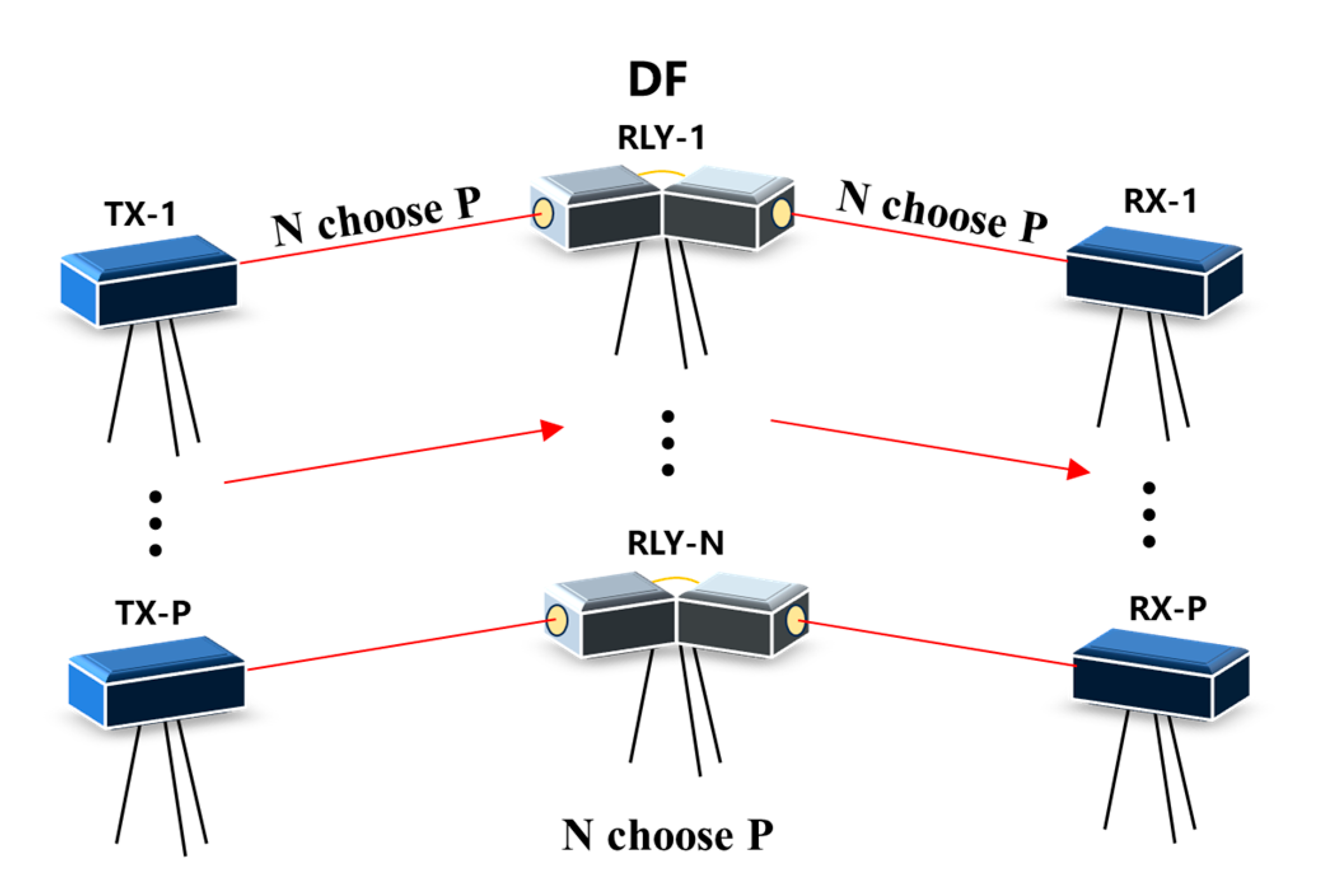
The system model of this paper is shown in Figure 1. In a multi-transceiver FSOC system with relays, there are P transmitting terminals (TX-1, …, TX-P), P receiving terminals (RX-1, …, RX-P), and N relay terminals (RLY-1, …, RLY-N). The red line represents the laser link. At any time, all the transmitting terminals will choose a different relay terminal as the relay node, which means that there are P parallel independent links in each time slot. In this paper, it is assumed that the relay terminals employ the DF method, and that all transmitting terminals and relay terminals adopt On–Off Keying (OOK) modulation in the NRZ format, chosen for its simple transceiver structure and balanced 0/1 signal characteristic, which simplify clock data recovery at the receiver. The Gaussian noise power between the transmit-relay and relay-receive terminals is and , respectively.
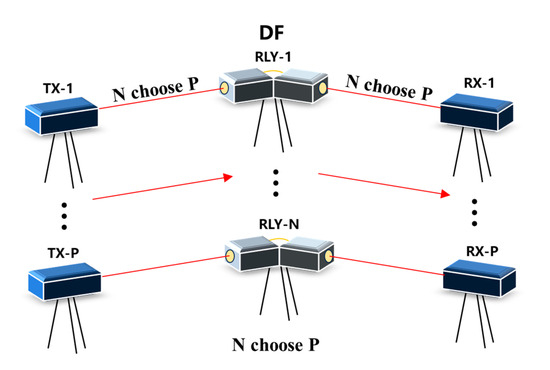
Figure 1.
Diagram of a multi-transceiver FSOC system with relays.
2.2. Malaga Turbulence and Pointing Errors
Before analyzing the probability density function (PDF) of channel fluctuations, considering pointing errors, it is essential to select an appropriate turbulence model. The log-normal, lognormal-Rician, and gamma-gamma models are among the most prominent [23]. However, the log-normal model is limited to scenarios with weak irradiance fluctuations. Although the lognormal-Rician model aligns well with experimental data, it lacks a closed-form solution for its integral and has inherent convergence issues. Alternatively, the gamma-gamma model is proposed as a practical substitute for the lognormal-Rician model, owing to its more manageable mathematical formulation. It is worth noting that Ref. [24] introduces the Malaga turbulence (M distribution), applicable to both plane and spherical waves across all turbulence conditions, ranging from weak to extremely strong in the saturation regime. This distribution unifies the log-normal and gamma-gamma models into a single closed-form expression, encompassing various models proposed for atmospheric optical communications. Consequently, the gamma-gamma and log-normal distributions are special cases of the Malaga model under different turbulence conditions [25]. The Mdistribution PDF of irradiance is expressed as follows:
where are the Malaga channel parameters. In Equation (1), Kν(·) is the modified Bessel function of the second kind and order ν.
Let represent the channel gain between the i-th () transmitting terminal and the j-th () relay terminal in the k-th time slot. Similarly, let represent the channel gain between the j-th () relay terminal and the i-th () receiving terminal in the k-th time slot. In this paper, atmospheric attenuation, turbulence fluctuation, and pointing errors are considered. Then, using the Malaga model, the PDF of the channel fluctuation with pointing errors can be expressed as follows:
where represents the Meijer’G function, is the path loss which obtains turbulence attenuation, geometric loss, and both transmission and reception losses. and represent the pointing error parameter.
2.3. Effect of Handoff Loss
Similarly to Ref. [21], is defined as the handoff loss during the handover of adjacent nodes. However, Ref. [21] only considers the case of a single transmitting terminal, and all relay nodes always point to the transmitting terminal and the receiving terminal, thus eliminating the problem of relay node-handover direction. In this paper, the issue of relay node-pointing switches needs to be additionally considered. As mentioned above, in the kth time slot, it is assumed that the relay node is selected for the i-th transmitting terminal to the i-th receiving terminal. Similarly, in the (k + 1)-th time slot, the relay node RX-i is selected for the i-th transmitting terminal to the i-th receiving terminal. Then, in the (k + 1)-th time slot, the handover loss from TX-i to and then to RX-i link should be calculated as follows:
where represents the direction of the relay node before the (k + 1)-th time. Therefore, considering the handover loss, the channel capacity in the k-th time slot should be expressed as follows:
where is the channel capacity of the link from TX-i to RX-i through the relay node in the k-th time slot under the premise of considering the handover loss. is the channel capacity of the link from TX-i to RX-i through the relay node in the k-th time slot without considering the handover loss. The relationship between the two is . Consider that in the k-th time slot, if the relay node is selected for the link from the i-th transmitting terminal to the i-th receiving terminal, the expression of is
The objective of this study is to maximize the average channel capacity in M time slots, namely
where represents the set of relay nodes selected in M time slots, that is, . From Equation (7), the system needs to carefully select relay nodes in each time slot because each selection will affect the handover loss in subsequent time slots, further impacting the final channel capacity. In the actual systems, the study cannot predict the channel state of subsequent time slots, but fortunately, the study can leverage reinforcement learning techniques to optimize the relay selection in each time slot by maximizing the characteristics of long-term cumulative reward functions.
As mentioned above, the primary objective of this paper is to maximize the average channel capacity of M time slots. Therefore, the cumulative channel capacity with a discount factor starting from time k needs to be defined:
where γ represents the discount factor, which ranges between 0 and 1. Therefore, the problem of maximizing the average channel capacity in M time slots can be transformed into the form of Equation (9)
3. The RLRS Algorithm
In reinforcement learning, the problem to be solved is typically modeled as an MDP. The MDP generally consists of four elements : the state space , the action space , the reward function at the current time , and the transition probability . The next state is only determined by the current state and the current action and is independent of previous states. In the relay selection model of this paper, since the transition probability is unknown, it can be modeled as an incomplete MDP, consisting of three elements . Correspondingly, ,, are defined as the state, action, and immediate reward functions at the k-th time slot, respectively. In the model of this paper, the specific contents of ,, are as follows:
- ■
- State : In any k-th time slot, state includes two parts: the pointing (including 2P + N elements) of all nodes in the (k-1)th time slot and the channel gain of the S-R link and R-D link in all current time slots (including 2PN elements).
- ■
- Action : In any k-th time slot, action represents the sequence number (including P elements) of the relay nodes selected for all transmitting nodes. There are possibilities in the action space. With , we can write any action into the form of a P-bit N-ary number, that is, .
- ■
- Immediate reward function : When action is performed under state , an immediate reward function will be obtained. This reward function is utilized to indicate whether action performed in the current state is beneficial.
Since action is written in the form of a P-bit N-ary number, the action space is expanded from dimension to dimension. In this case, there will be situations where multiple transmitting nodes select the same relay. To avoid this, we define as follows:
In reinforcement learning, the agent maximizes the cumulative reward function with a discount factor by learning the optimal strategy. In order to evaluate the performance of the strategy, the Q-value is typically introduced as a metric, defined as follows: .When the state and action spaces are small enough, the common reinforcement learning approach is the Q-table method. By listing all actions for each state, the Q-value table of each action-–state pair is obtained, and the action with the largest Q-value is selected as the optimal strategy. However, in this paper, the state space is continuous, and the action space is also very large, making it impossible to list all Q-tables. Therefore, a DQN is adopted. In a DQN, a neural network is used to simulate the action value function, allowing it to handle each action value function in high-dimensional state space and output the maximum value function.
Inspired by Ref. [16], this paper also adopts a Dueling-DQN network structure and proposes an RLRS algorithm. However, the action space, state space, and reward function in this paper differ from those in Ref. [16]. The overall structure of this paper’s RLRS algorithm is shown in Figure 2. The RLRS algorithm includes two neural networks—one is an online neural network, the other a target neural network, both with the same network structure. The input layer, hidden layer, and output layer structures of the RLRS algorithm differ slightly from those of conventional DQNs. In the RLRS structure, the layer before the output layer is divided into two parts: the state value part and the action advantage part . They are expressed in Equation (11).
where represents the weight threshold of the other layers except the last layer in the online network. and , respectively, represent the weight threshold of the state-value part and the action-advantage-value part in the online network. Since the target network has the same structure as the online network, the corresponding parameters , , and in the target network can be defined. Similarly, the parameters of the online network can be completely determined by , , and .
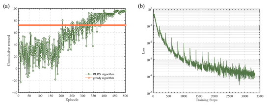
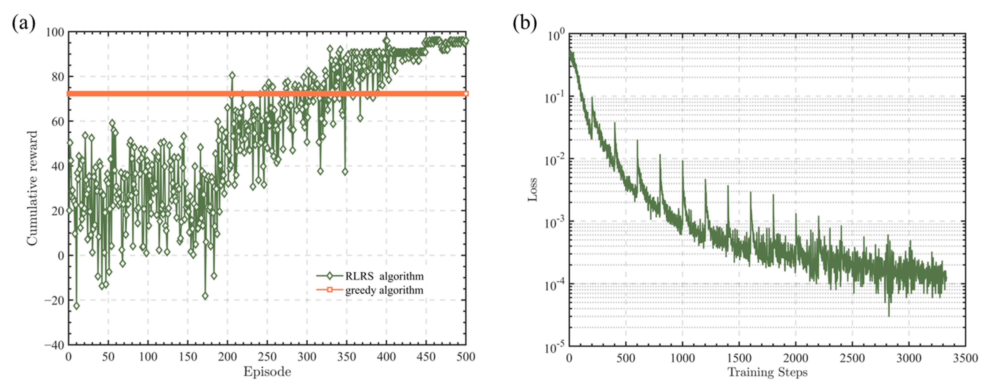
Figure 2.
Performance of an RLRS algorithm in 10 time slots. (a) Curves of cumulative reward. (b) Curve of loss function.
The input layer of the RLRS algorithm has 2PN + 2P + N neurons, corresponding to the dimensions of the state space, and the output layer has N elements, corresponding to the dimensions of the expanded action space. As mentioned earlier, the output of the online network represents the Q-value of the optimal state–action pair in the current strategy, which can be expressed as follows:
where represents the number of elements in . Similarly, represents the output of the target network when the input is and the selection action is . In any k-th time slot, in the process of selecting an action , a - greedy approach is adopted, that is, the network will arbitrarily select an action in the state space with the probability of . Otherwise, it will select the action with the maximum Q-value, as shown in Equation (13).
In the k-th time slot, based on the state , after selecting , the immediate reward of k-th time slot will be obtained, and then it enters the next state . At this point, it yields a set of empirical values , which can be put into experience pool . The experience pool has a first-in, first-out structure and can store elements. If the experience pool is not full, the experience value will be directly stored in the experience pool; if the experience pool is already full, the earliest stored experience will be removed, and the new experience value will be stored in the experience pool .
The online network is updated first,
where ,, and represent the gradient values of the loss function with respect to 、, and , respectively. represents the learning rate of the online network. After updating the online network, the target network is subsequently updated. Assuming the learning rate of the target network is , the network parameters are updated as follows:
The pseudocode diagram of the proposed RLRS algorithm is depicted in Algorithm 1.
| Algorithm 1. The pseudocode diagram of the proposed RLRS algorithm. | |
| Input: The FSOC system simulator and its parameters. Output: Optimal action of each time slot. | |
| 1: | Initialize experience replay memory . |
| 2: | Initialize , and with random weights and initialize , and . |
| 3: | Initialize the minibatch size with X. |
| 4: | FOR episode in DO |
| 5: | Observe the environment initial state . |
| 6: | FOR = 1 to K DO |
| 7: | Select a relay selection action by Equation (11), and execute action . |
| 8: | IF there is same element in |
| 9: | Calculate immediate reward . |
| 10: | ELSE |
| 11: | Calculate immediate reward . |
| 12: | Obtain next state and store transition data in replay memory . |
| 13: | IF is full |
| 14: | Sample a random minibatch of X sets of transition data from . |
| 15: | Update the online network by (13). |
| 16: | Update the target network by (14). |
| 17: | END FOR |
| 18: | END FOR |
4. Simulation Results
In this section, the performance simulation of the RLRS algorithm is presented, and the simulation parameters are shown in Table 1. As a comparison, a greedy algorithm is utilized as a reference to demonstrate the advantages and effectiveness of the proposed RLRS algorithm.

Table 1.
Simulation parameters.
According to the above parameters and pseudo-code, the following simulation is obtained. Figure 2a,b shows the cumulative reward curve and the loss function curve for a time slot number of 10. Figure 2a shows the training results across different episodes. The training process can be roughly divided into three parts: the experience pool storage part, the parameter update part, and the training completion part. Before the experience pool is full, the cumulative reward curve fluctuates without a clear upward trend. Once the experience pool is full, the system extracts experiences from the pool and utilizes the mini-batch method for parameter updates. At this point, the cumulative reward curve shows an overall upward trend. After the 400th episode, the cumulative reward value tends to stabilize, and the stable cumulative reward value is superior to the performance of the greedy algorithm. The loss function curve in Figure 2b shows a periodic trend of decline, indicating the convergence of the algorithm.
Figure 3a,b shows the cumulative reward curve and the loss function curve for a time slot number of 50. Overall, the curve trends in Figure 3 are almost identical to those in Figure 2. This also demonstrates that the proposed RLRS algorithm in this paper can converge under different time slot conditions and outperforms the greedy algorithm.
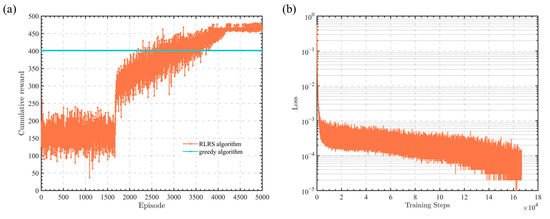
Figure 3.
Performance of RLRS algorithm in 50 time slots. (a) Curves of cumulative reward. (b) Curve of loss function.
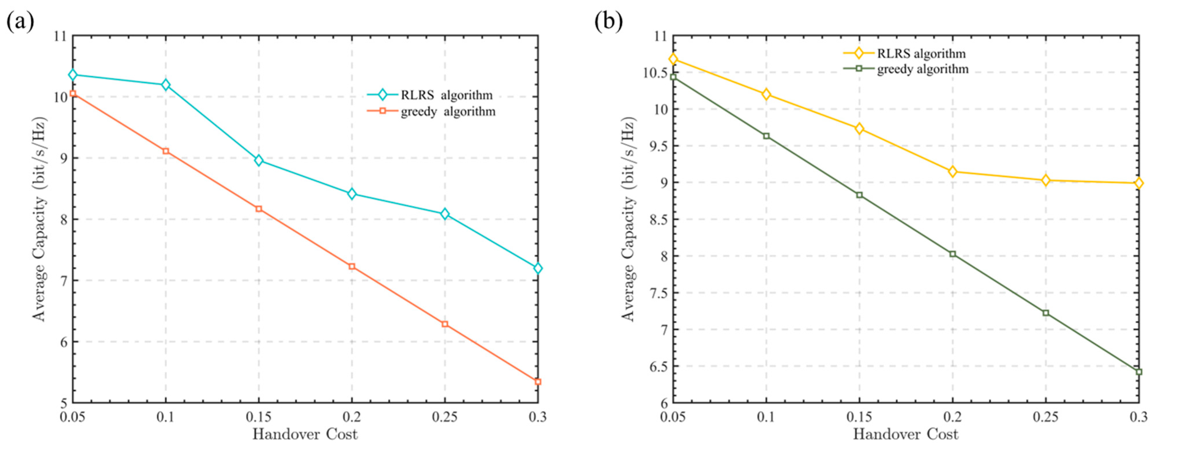
Figure 4 presents the average channel capacity curves under different handover loss conditions. Figure 4a,b describes the cases of 10 time slots and 50 time slots. As can be seen from Figure 4a,b, the proposed RLRS algorithm in this paper consistently outperforms the greedy algorithm under various handover loss conditions. Additionally, as the handover loss increases, the gap between the two algorithms gradually widens, with the RLRS algorithm providing at least a 2.47% improvement in channel capacity. This is because the conventional greedy algorithm only selects the relay node with the largest channel gain without considering handover loss. As a result, when the handover loss increases, its capacity decreases linearly. In contrast, the proposed RLRS algorithm in this paper takes both handover loss and channel gain into account, so as to maximize the long-term rewards of relay selection in each time slot.
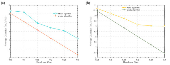
Figure 4.
Average channel capacity versus different handover loss. (a) 10 time slots. (b) 50 time slots.
Figure 5 shows the average capacity of the RLRS algorithm and the traditional greedy algorithm when fog’s influence is considered. According to the Kruise formula, the attenuation due to fog (dB/km) is defined as follows:
where is the wavelength (in nm), V represents the visibility (in km). q is a parameter that depends on the particle size distribution of scattering particles, given as follows:

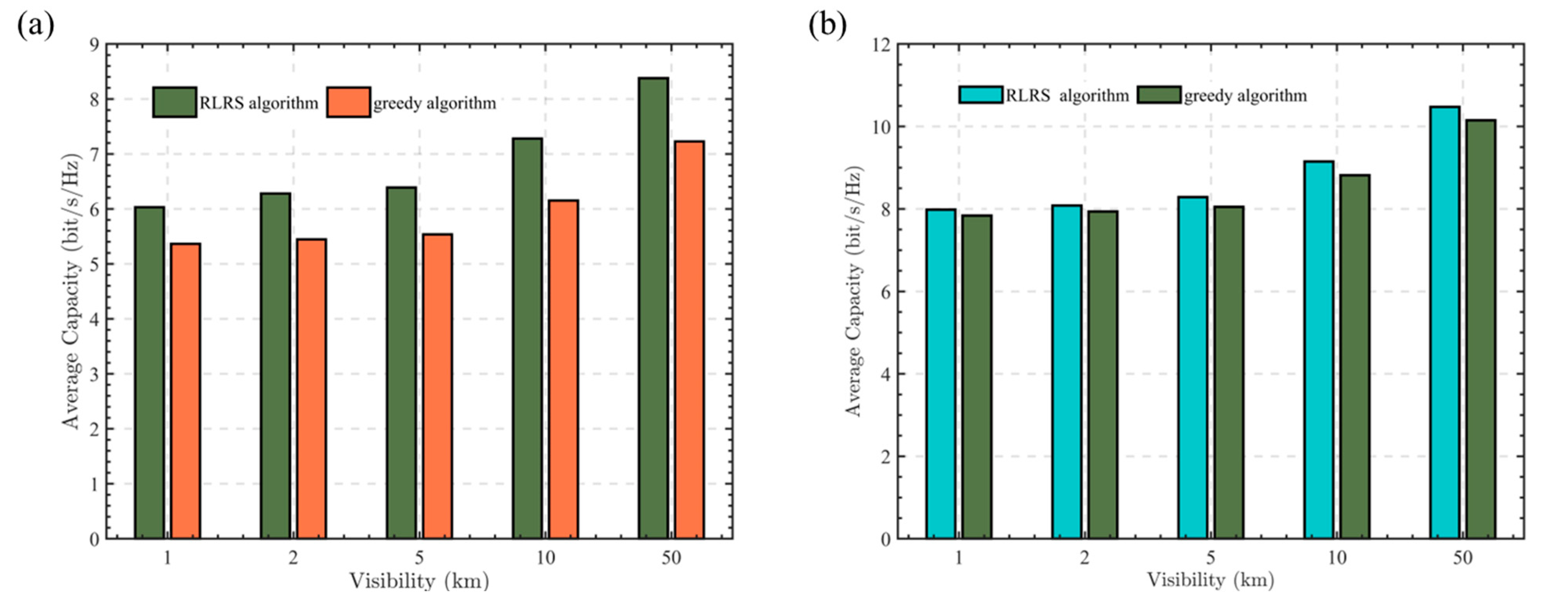
Figure 5.
Average capacity of RLRS and greedy algorithm under Malaga and Gamma-Gamma turbulence with fog. (a) Average capacity under Malaga turbulence with fog. (b) Average capacity under Gamma-Gamma turbulence with fog.
This paper selected the wavelength as 1550 nm. The visibility is set to 1 km, 2 km, 5 km, 10 km, 50 km, respectively. As shown in Figure 5a, which illustrates Malaga turbulence, the average capacity increases with visibility. This is due to the fact that greater visibility results in reduced attenuation. Figure 5b illustrates Gamma-Gamma turbulence with , , where the Malaga turbulence can reduce to Gamma-Gamma turbulence with and . As can be seen from Figure 5a,b, the RLRS algorithm always performs better than the traditional greedy algorithm. Besides the situation of weak turbulence, which has a larger average capacity in both the RLRS and greedy cases, Figure 5a,b also show that the RLRS algorithm performs more effectively under strong turbulence. This is because strong turbulence can cause significant variations in channel gains across multiple potential links. Consequently, during relay selection, the difference in system performance between high-quality and low-quality relays becomes more pronounced, leading to a more noticeable improvement in system performance with the RLRS algorithm.
5. Conclusions
This paper proposes a relay selection algorithm to mitigate the capacity degradation caused by atmospheric turbulence, where there are N transmitting nodes (and N receiving nodes) and P relay nodes. We also consider the handover loss caused by the handover process of different relay nodes. The RLRS algorithm is proposed based on a Dueling DQN structure to maximize the average channel capacity. In the implementation of the RLRS algorithm, the actions are encoded in a multi-digit format, and a reward function with a penalty term is designed based on whether the multi-digit actions are repeated. Finally, through simulation comparison, the RLRS algorithm proposed in this paper is shown to be superior to the greedy comparison algorithm, which can enhance the channel capacity by at least 2.47%, with the gap increasing as handover loss rises. Moreover, under stronger turbulence, the RLRS algorithm demonstrates a noticeable improvement in channel capacity, further validating its effectiveness in combating the capacity loss induced by turbulence. Therefore, this study not only provides a reference design scheme for the relay FSOC system to further fight against turbulence, but also demonstrates the potential of reinforcement learning in improving channel capacity, which offers new insights and directions for future high-performance communication system design.
Author Contributions
Conceptualization, X.S. and Z.L.; Methodology, X.S.; Software, Z.L.; Formal analysis, X.S.; Writing—original draft, X.S.; Writing—review and editing, Z.L.; Supervision, Y.W. All authors have read and agreed to the published version of the manuscript.
Funding
This research received no external funding.
Institutional Review Board Statement
Not applicable.
Informed Consent Statement
Not applicable.
Data Availability Statement
The raw data supporting the conclusions of this article will be made available by the authors on request.
Conflicts of Interest
The authors declare no conflict of interest.
References
- Al-Kinani, A.; Wang, C.X.; Zhou, L.; Zhang, W. Optical Wireless Communication Channel Measurements and Models. IEEE Commun. Surv. Tutor. 2018, 20, 1939–1962. [Google Scholar] [CrossRef]
- Wang, T.; Lin, P.; Dong, F. Progress and Prospect of Space Laser Communication Technology. Strateg. Study CAE 2020, 22, 92–99. (In Chinese) [Google Scholar] [CrossRef]
- Khalighi, M.A.; Uysal, M. Survey on free space optical communication: A communication theory perspective. IEEE Commun. Surv. Tutor. 2014, 16, 2231–2258. [Google Scholar] [CrossRef]
- Safari, M.; Uysal, M. Relay-assisted free-space optical communication. IEEE Trans. Wireless Commun. 2008, 7, 5441–5449. [Google Scholar] [CrossRef]
- Chatzidiamantis, N.; Michalopoulos, D.; Kriezis, E.; Karagiannidis, G.; Schober, R. Relay Selection Protocols for relay-assisted Free Space Optical systems. Opt. Commun. Netw. 2013, 5, 92–103. [Google Scholar] [CrossRef]
- Zhang, Z.; Zhang, P.; Yu, H. Research on polar laser communication based on relay system. Opt. Commun. Technol. 2021, 45, 56–58. (In Chinese) [Google Scholar]
- Boluda-Ruiz, R.; Garcia-Zambrana, A.; Castillo-Vazquez, B. Ergodic capacity analysis of decode-and-forward relay-assisted FSO systems over alpha–Mu fading channels considering pointing errors. IEEE Photonics J. 2016, 8, 1–11. [Google Scholar] [CrossRef]
- Abou-Rjeily, C.; Noun, Z.; Castillo-Vazquez, B. Impact of inter-relay cooperation on the performance of FSO systems with any number of relays. IEEE Trans. Wirel. Commun. 2016, 15, 3796–3809. [Google Scholar] [CrossRef]
- Zhang, R.; Zhang, W.; Zhang, X. Research status and development trend of high earth orbit satellite laser relay links. Laser Optoelectron. Prog. 2021, 58, 9–21. (In Chinese) [Google Scholar]
- Taher, M.; Abaza, M.; Fedawy, M. Relay selection schemes for FSO communications over turbulent channels. Appl. Sci. 2019, 9, 1281. [Google Scholar] [CrossRef]
- Tan, Y.; Liu, Y.; Guo, L.; Han, P. Joint relay selection and link scheduling in cooperative free-space optical system. Opt. Eng. 2016, 55, 111604. [Google Scholar] [CrossRef]
- Ben, H. Round, Robin, Centralized and distributed relay selection for free space optical communications. Wirel. Pers. Commun. 2019, 108, 51–66. [Google Scholar] [CrossRef]
- Abou-Rjeily, C. Improved Buffer-Aided Selective relaying for free space optical cooperative communications. IEEE Trans. Wirel. Commun. 2022, 21, 6877–6889. [Google Scholar] [CrossRef]
- Palitharathna, S.; Godaliyadda, I.; Herath, R. Relay-assisted optical wireless communications in turbid water. In Proceedings of the International Conference on Under Water Networks and Systems, Shenhen, China, 3–5 December 2018; pp. 1–5. [Google Scholar] [CrossRef]
- Gao, Z.; Eisen, M.; Ribeiro, A. Resource Allocation via Model-Free Deep Learning in Free Space Optical Communications. IEEE Trans. Commun. 2021, 70, 920–934. [Google Scholar] [CrossRef]
- Le-Tran, M.; Vu, H.; Kim, S. Performance Analysis of Optical Backhauled Cooperative NOMA Visible Light Communication. IEEE Trans. Veh. Technol. 2021, 70, 12932–12945. [Google Scholar] [CrossRef]
- Dang, H.; Liang, Y.V.; Wei, L. Enabling Relay Selection in Cooperative Networks by Supervised Machine Learning. In Proceedings of the Eighth International Conference on Instrumentation & Measurement, Computer, Communication and Control (IMCCC), Harbin, China, 19–21 July 2018; pp. 1459–1463. [Google Scholar] [CrossRef]
- Dang, S.; Tang, J.; Li, J.; Wen, M.; Abdullah, S. Combined relay selection enabled by supervised machine learning. IEEE Trans. Veh. Technol. 2021, 70, 3938–3943. [Google Scholar] [CrossRef]
- Kapsis, T.; Lyras, K.; Panagopoulos, D. Optimal Power Allocation in Optical GEO Satellite Downlinks Using Model-Free Deep Learning Algorithms. Electronics 2024, 13, 647. [Google Scholar] [CrossRef]
- Su, Y.; Li, W.; Gui, M. Optimal Cooperative Relaying and Power Control for IoUT Networks with Reinforcement Learning. IEEE Internet Things J. 2021, 8, 791–801. [Google Scholar] [CrossRef]
- Su, Y.; Lu, X.; Zhao, Y.; Huang, L.; Du, X. Cooperative communications with relay selection based on deep reinforcement learning in wireless sensor networks. IEEE Sens. J. 2019, 19, 9561–9569. [Google Scholar] [CrossRef]
- Gao, S.; Li, Y.; Geng, T. Deep reinforcement learning-based relay selection algorithm in free-space optical cooperative communications. Appl. Sci. 2022, 12, 4881. [Google Scholar] [CrossRef]
- Jurado-Navas, A.; Garrido-Balsells, J.; Paris, J.; Castillo-Vázquez, M. Impact of pointing errors on the performance of generalized atmospheric optical channels. Opt. Express. 2012, 20, 12550–12562. [Google Scholar] [CrossRef] [PubMed]
- Jurado-Navas, A.; Garrido-Balsells, J.; Paris, J.; Puerta-Notario, A. A unifying statistical model for atmospheric optical scintillation. In Numerical Simulations of Physical and Engineering Processes; Intech: Rijeka, Croatia, 2011; Volume 181, pp. 181–205. [Google Scholar] [CrossRef]
- Ansari, I.S.; Yilmaz, F.; Alouini, M.S. Performance analysis of free-space optical links over Málaga turbulence channels with pointing errors. IEEE Trans. Wirel. Commun. 2015, 15, 91–102. [Google Scholar] [CrossRef]

Disclaimer/Publisher’s Note: The statements, opinions and data contained in all publications are solely those of the individual author(s) and contributor(s) and not of MDPI and/or the editor(s). MDPI and/or the editor(s) disclaim responsibility for any injury to people or property resulting from any ideas, methods, instructions or products referred to in the content. |
© 2024 by the authors. Licensee MDPI, Basel, Switzerland. This article is an open access article distributed under the terms and conditions of the Creative Commons Attribution (CC BY) license (https://creativecommons.org/licenses/by/4.0/).