Abstract
The accurate transformation of multi-camera 2D coordinates into 3D coordinates is critical for applications like animation, gaming, and medical rehabilitation. This study unveils an enhanced multi-camera calibration method that alleviates the shortcomings of existing approaches by incorporating a comprehensive cost function and Adaptive Iteratively Reweighted Least Squares (AIRLS) optimization. By integrating static error components (3D coordinate, distance, angle, and reprojection errors) with dynamic wand distance errors, the proposed comprehensive cost function facilitates precise multi-camera parameter calculations. The AIRLS optimization effectively balances the optimization of both static and dynamic error elements, enhancing the calibration’s robustness and efficiency. Comparative validation against advanced multi-camera calibration methods shows this method’s superior accuracy (average error 0.27 ± 0.22 mm) and robustness. Evaluation metrics including average distance error, standard deviation, and range (minimum and maximum) of errors, complemented by statistical analysis using ANOVA and post-hoc tests, underscore its efficacy. The method markedly enhances the accuracy of calculating intrinsic, extrinsic, and distortion parameters, proving highly effective for precise 3D reconstruction in diverse applications. This study represents substantial progression in multi-camera calibration, offering a dependable and efficient solution for intricate calibration challenges.
1. Introduction
The transformation of multi-camera 2D coordinates into accurate 3D coordinates is fundamental for applications in computer vision such as animation, gaming, sports analysis, and medical rehabilitation [1,2,3,4]. Optical motion capture systems, which depend on this transformation for precise movement capture and reconstruction, require accurate camera calibration. This involves determining the cameras’ intrinsic and extrinsic parameters, which are crucial for forming projection matrices that convert 2D image coordinates into precise 3D world coordinates [5]. Despite extensive research, achieving high accuracy and user convenience in multi-camera calibration continue to pose substantial challenges [4,6].
Traditional multi-camera calibration methods are generally divided into two types: static, which uses a fixed object proportional to the 3D tracking space, and dynamic, which employs a moving object. Static methods, such as the Direct Linear Transformation (DLT) proposed by Abdel-Aziz et al. [7], calculate camera parameters by extracting optimal transformation matrices between the 3D coordinates of markers on the calibration object and their corresponding 2D coordinates in each camera’s image plane. The primary advantage of static calibration is its ability to provide robust and accurate calculations of intrinsic and extrinsic camera parameters within the 3D tracking space fully covered by the calibration object. This accuracy is achieved because precise spatial information and constraints allow for the derivation of exact transformation matrices describing the 2D-to-3D transformations within the limits of the available spatial data. However, a key drawback is the strong dependence on the scale and intricacy of the 3D tracking space, necessitating a calibration object of proportional size and complexity [8]. Consequently, static calibration methods cannot guarantee accuracy outside the area covered by the object. To achieve a large 3D tracking space using a multi-camera system, a larger object with a substantial number of optical markers is required [4,8], making the setup process labor-intensive and time-consuming.
Dynamic calibration methods address the primary limitation of static calibration by eliminating the need for a calibration object that matches the size and complexity of the desired 3D tracking space. These methods use a moving calibration object, enabling the quicker and easier adjustment of the 3D tracking space without the need to develop a specialized static object for each required 3D tracking area. Commonly used moving calibration objects include rigid bars or T-wands, typically equipped with a smaller number of markers (usually two [2,3,9,10,11]) with a known distance between them. Using moving calibration object data eliminates the need for extensive calibration setup, significantly reducing the overall calibration time and labor required. This leads to a more rapid and convenient calibration process. For example, Borghese et al. [12] introduced a method using a rigid bar for dynamic calibration, leveraging the motion of the bar to optimize camera parameters. Similarly, Mitchelson et al. [9] proposed a T-wand-based calibration method, particularly suited for multiple camera studios, which simplifies the setup process and reduces the overall calibration time to approximately 5 min, compared to several hours for static calibration. However, dynamic methods face significant limitations, including reduced accuracy and consistency [3]. These methods typically rely on a geometrically simple moving calibration object, with the distance between markers serving as the primary spatial constraint. Due to the simplicity of using a rigid bar or T-wand with fewer markers, the initial estimation of camera parameters may lack precision, as it heavily depends only on the multi-view geometry of marker image locations and the known marker distance. This can make it difficult to effectively minimize the distance error between markers during iterative multi-camera parameter refinement, potentially leading to a local minimum and resulting in a loss of overall calibration accuracy [3,10].
The combination of the limitations and advantages in static and dynamic calibration methods has led to the development of hybrid approaches that aim to leverage the strengths of both while mitigating their respective drawbacks. Hybrid methods use a simpler, easy-to-install static calibration object, such as an L-frame or a three-axis frame, to calculate accurate initial multi-camera parameters using known spatial constraints like the 3D coordinates of optical markers on the static calibration frame. Combining this with movements within the desired calibration area using a moving calibration object, such as a calibration wand, allows for the expansion of the tracking area to the desired size. The further optimization of multi-camera parameters with a combination of clear spatial constraints from the static calibration object and tracking data within the tracking area using the moving calibration object helps avoid the local minimum problem of the dynamic calibration method. This is achieved by using accurate initial parameters calculated during the static calibration process with a static calibration object with known spatial constraints. Ultimately, this method enables the more precise calculation of multi-camera parameters within the desired tracking area by effectively reducing both static errors (through spatial constraints of the static calibration object) and dynamic errors (through tracking data from the dynamic object with simple constraints). For example, Uematsu et al. [13] utilized an L-frame for static calibration and combined static reprojection error with dynamic distance errors between wand markers for optimization. Pribanić et al. [10] used an orthogonal wand triad for static calibration and a wand for dynamic calibration, improving calibration accuracy by calculating fundamental and essential matrices for each camera. Similarly, Shin et al. [3] employed a three-axis frame and wand, considering both the 3D coordinate errors of spherical markers for static error and the distance errors between spherical markers during wanding for dynamic error. These methods optimize camera parameters using a combined cost function, thereby enhancing user convenience and accuracy.
Despite advancements, existing hybrid methods combining static and dynamic calibration have notable limitations. A significant drawback is the limited use of multiple error components in static calibration, typically focusing only on 3D coordinates or reprojection errors while neglecting crucial factors like distance and angular errors [14,15]. Incorporating 3D coordinate errors ensures precise spatial localization, reducing deviations in reconstructed 3D marker positions and enhancing the accuracy of multi-view triangulation [3]. Distance errors maintain correct scaling in the 3D space by enforcing consistency in known distances between markers, preventing distortions [10]. Angle errors preserve geometric relationships among markers, essential for maintaining the structural integrity of the setup [16]. Reprojection errors correct discrepancies between observed image points and their projections, crucial for addressing lens distortions and quantification inaccuracies, thus preventing these errors from affecting 3D reconstructions [13,17]. The integration of these components forms a comprehensive constraint system, minimizing biases in the calibration process and mitigating calibration and 3D reconstruction errors [3,14,16]. The addition of dynamic error through wand distance error further refines this framework, accommodating temporal variations and improving tracking accuracy during dynamic calibration, ultimately reducing 3D triangulation errors [3,10,13,18]. Existing hybrid methods often excluded multiple error components in static calibration due to several factors. The complexity of simultaneously optimizing diverse error components posed significant computational challenges, risking overfitting to specific errors, particularly in systems with limited computational resources [16]. Furthermore, the theoretical frameworks and software tools available at the time were typically tailored to specific error metrics, making it challenging to integrate a comprehensive cost function covering all error types [13]. As a result, many methods favored simplified calibration approaches [10,14,15,16,17,18,19], which, while sufficient for certain applications, did not fully leverage the potential of all error components, limiting their overall calibration accuracy [3,10,14]. Additionally, hybrid methods often encountered issues due to the unequal data representation between static and dynamic errors, leading to a tendency towards overfitting to dynamic errors, which increased static errors and resulted in suboptimal calibration [14,15].
Therefore, this study aims to overcome the limitations, such as the limited use of error components and the overfitting risk of previous hybrid calibration methods, by developing a comprehensive cost function and employing a balanced optimization approach. The proposed method integrates 3D coordinate, distance, angle, and reprojection errors in static calibration, alongside dynamic wand distance error, to provide a holistic framework for minimizing calibration errors. The optimization is conducted using the adaptive iteratively reweighted least squares (AIRLS) method proposed in this research, which assigns differential weights to static and dynamic errors, ensuring that neither dominates the optimization process, thereby preventing overfitting and achieving a more accurate calibration. This optimization method’s effectiveness was compared with those of previously developed optimization techniques, such as Sparse Bundle Adjustment (SBA) [20,21] and the Levenberg–Marquardt (LM) method [22,23]. In addition, the effectiveness of the proposed method was validated against leading-edge and high-precision multi-camera calibration techniques, including normalized DLT [24,25] and hybrid methods from related research, using commercial calibration wands with marker distances of 390 mm and 500 mm. The evaluation included metrics such as average distance error, standard deviation, minimum and maximum errors, and statistical significance assessed through ANOVA and post-hoc tests. The proposed method retains the simplicity of the calibration process and the rapid setup characteristic of combined methods while significantly enhancing accuracy in 3D reconstruction. These advantages make the proposed method particularly suitable for optical motion capture systems, robotics, surgical navigation systems and other applications requiring precise 3D reconstruction and tracking.
2. Materials and Methods
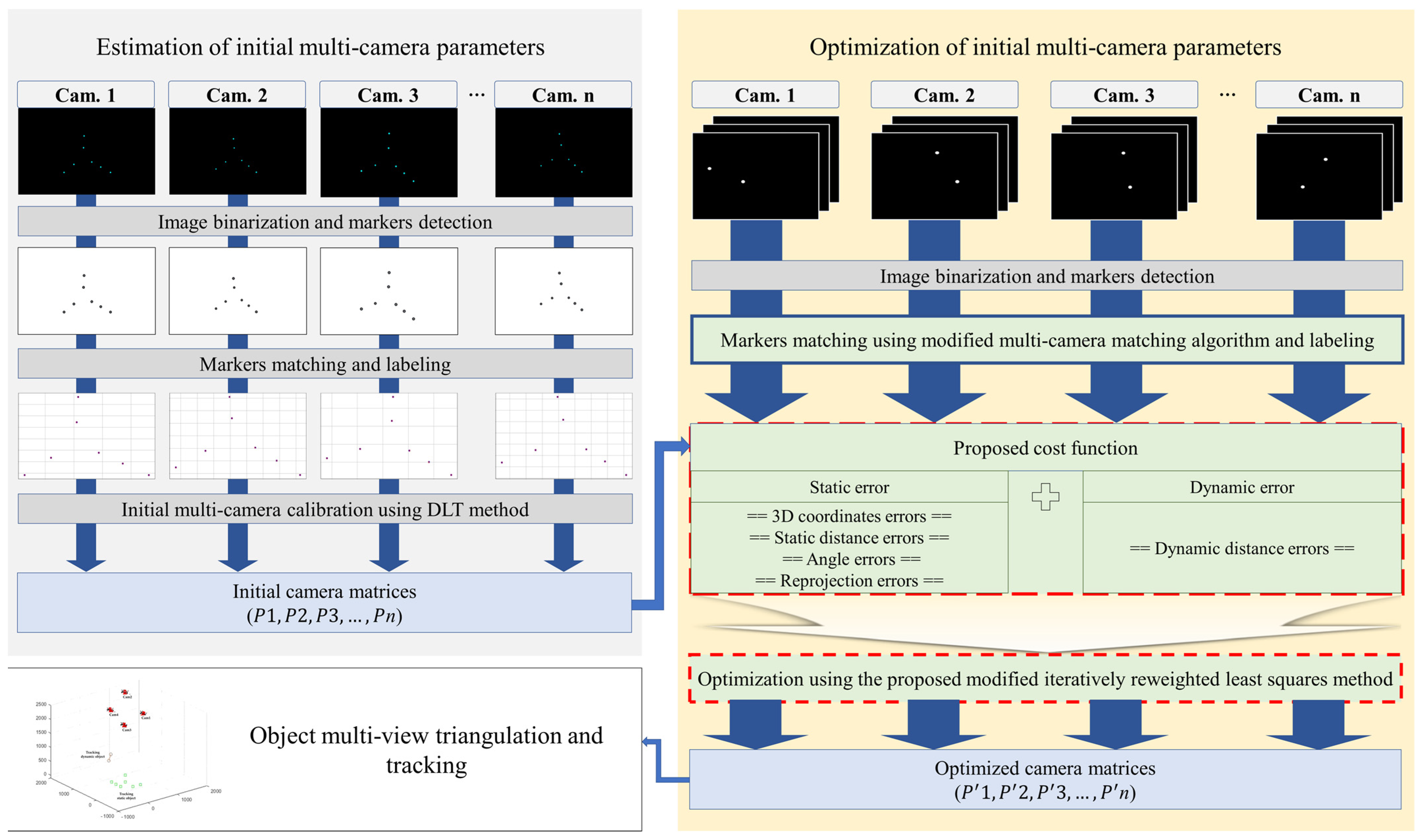
The proposed multi-camera calibration method integrates static and dynamic processes, enhancing both accuracy and usability. Initially, images of a three-axis calibration frame are synchronously acquired from all cameras. These images undergo binary conversion; markers are identified, matched, and labeled in accordance with the structure of the three-axis frame. Using normalized DLT, initial camera matrices are derived. Subsequently, a calibration wand is employed to gather approximately 1000 frames of data, which are then binarized; markers are detected and matched utilizing a proposed modified algorithm. A comprehensive cost function is formulated, incorporating static errors (3D coordinate, distance, angle, and reprojection errors) and dynamic errors (distance errors from wanding data). The AIRLS method optimizes the camera matrices, ensuring a balance between static and dynamic errors. The final intrinsic, extrinsic, and distortion parameters for each camera are extracted from the optimized matrices, facilitating precise multi-view triangulation and tracking. By integrating multiple error components, balanced optimization, and a robust matching algorithm, this method significantly enhances both accuracy and robustness. Figure 1 illustrates the detailed workflow of the proposed method.
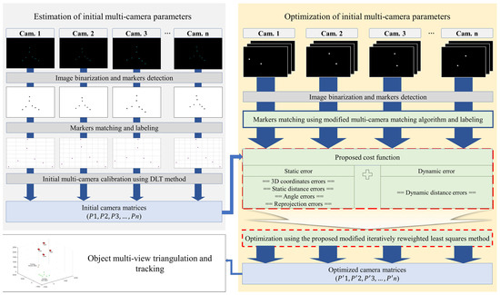
Figure 1.
Workflow of the proposed optimized multi-camera calibration process.
2.1. Experiments
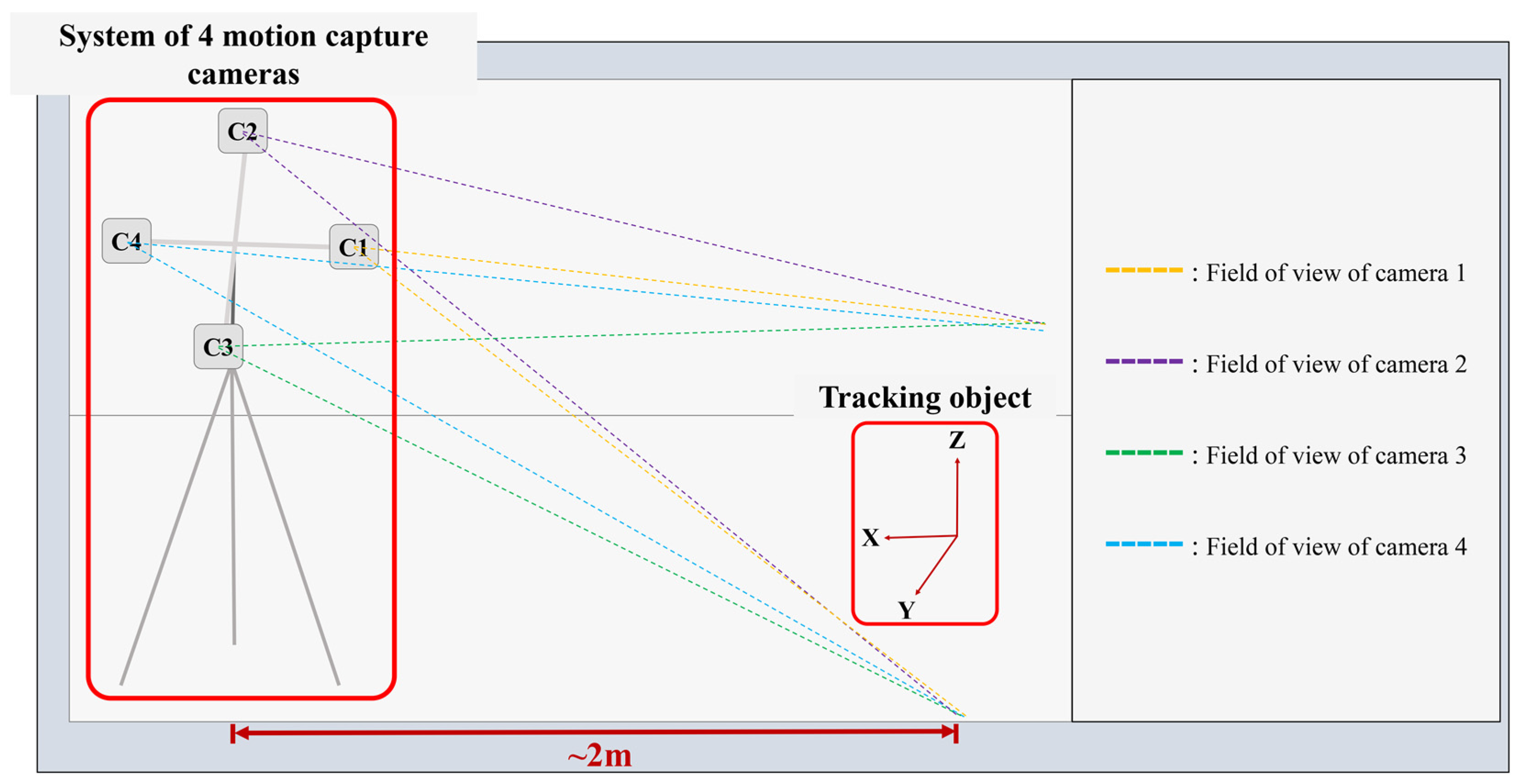
In this experiment, we utilized four CMOS cameras (OptiTrack FLEX 13; Natural Point, Corvallis, OR, USA) synchronized using a synchronization module (OptiHub2; Natural Point, Corvallis, OR, USA). The cameras were mounted on a custom-built multi-camera stand in a cross-axis configuration, with each camera positioned approximately 1 m apart to ensure a sufficient field of view for object tracking. Each camera featured a resolution of 1280 × 1024 pixels and operated at a frame rate of 120 Hz. The activities of multi-camera calibration and object tracking were conducted approximately 2 m from the center of the multi-camera stand, as depicted in Figure 2.
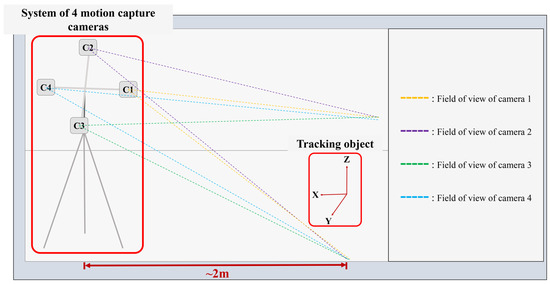
Figure 2.
Experimental setup.
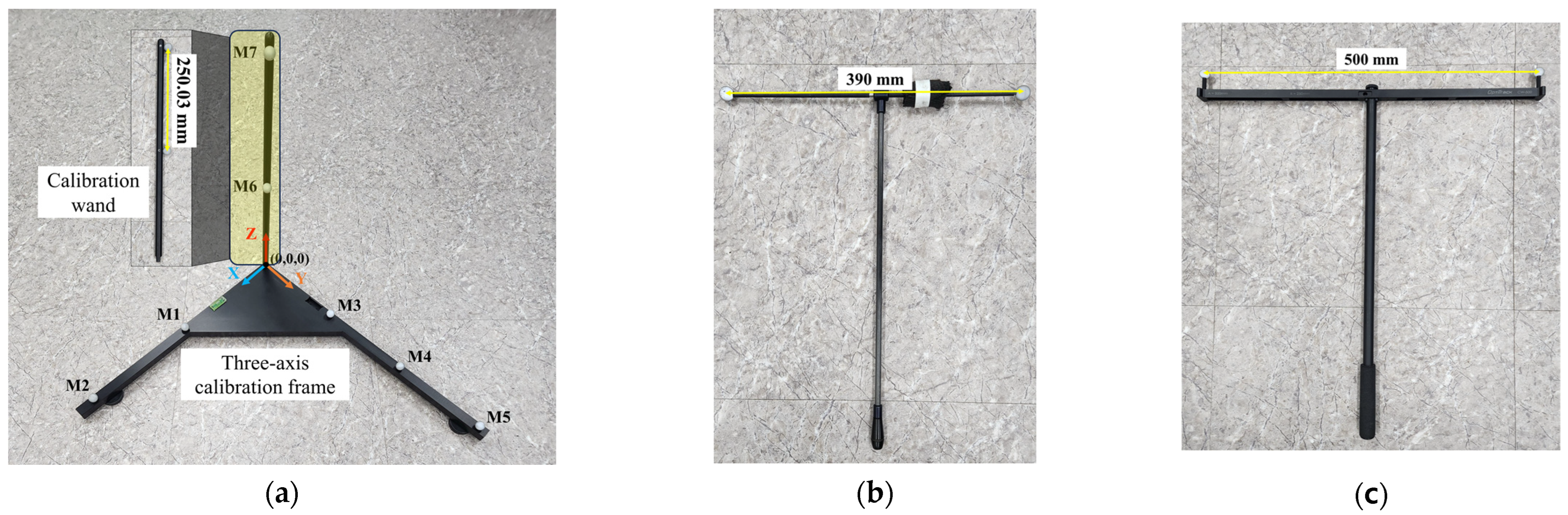
For the static calibration process, a three-axis calibration frame was used to estimate the initial multi-camera parameters. This frame, depicted in Figure 3a, included seven spherical optical markers with accurately measured 3D coordinates relative to the origin. These measurements were obtained using a 3D coordinate measuring machine (VICTOR101208; Dukin, Daejeon, Korea) with an average measurement error of 3.2 μm. The coordinates of the markers were as follows: two markers along the X-axis at (261.0510, −0.0730, 8.9900) and (511.0730, −0.1100, 8.7910); three markers along the Y-axis at (−0.0340, 210.9900, 9.0550), (0.1910, 411.0360, 9.0240), and (0.1210, 610.9330, 9.2030); and two markers along the Z-axis at (11.7680, 12.2170, 249.0830) and (11.5120, 12.7440, 499.1100). Each camera in the multi-camera system synchronously captured a frame of this calibration frame, ensuring all seven markers were within view. The Z-axis of the calibration frame featured a locking mechanism, allowing its detachment and use as a calibration wand. Approximately 1000 frames of wanding data were collected using this wand during dynamic calibration. These data were utilized to optimize the initial multi-camera parameters through the proposed optimization method, leveraging the known real-world distance between the centers of the two spherical markers on the wand.
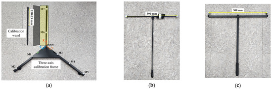
Figure 3.
Calibration and validation tools: (a) three-axis calibration frame employed for initial multi-camera parameter estimation and calibration wand used to optimize the initial parameters; (b) 390 mm commercial calibration wand employed for validation tracking data collection; (c) 500 mm commercial calibration wand employed for validation tracking data collection.
For further evaluation and validation of the proposed algorithm, tracking data were gathered using commercial motion capture system wands, such as the 390 mm commercial calibration wand (Vicon Motion Systems, Oxford, UK), illustrated in Figure 3b, with a marker center distance of 390 mm, and the 500 mm commercial calibration wand (Natural Point, Corvallis, OR, USA), illustrated in Figure 3c, with a marker center distance of 500 mm. The validation data consisted of approximately 1000 frames, with each trial being repeated five times to confirm the robustness of the results.
2.2. Estimation of Initial Multi-Camera Parameters
The process of estimating the initial camera parameters for each camera in the multi-camera system involved several detailed steps, utilizing a variety of computer vision and mathematical techniques as outlined below.
The initial step involves the binarization and detection of the u, v coordinates of markers on the three-axis calibration frame. This process includes converting the images to grayscale and applying Gaussian blurring [26] to reduce noise. A global thresholding method using Otsu’s method [27] is applied to create a binary image. Morphological operations such as closing are then performed to close gaps and remove small blobs using a kernel. The contours within the binary image are detected using the Suzuki-Abe method [28]. The centroids of these contours are calculated using image moments, specifically the spatial moments , , and , with the centroid coordinates defined by and . These centroid positions are then refined with sub-pixel accuracy using an iterative corner refinement algorithm based on minimizing the intensity variance within a window around each centroid.
Markers were automatically matched and labeled using the structural features of the three-axis calibration frame. This was achieved by sorting the detected markers based on their vertical positions (u-coordinates) to identify markers along the Z-axis. The two markers with the highest u-values were identified as the Z-axis markers. If , then Marker 6 is the lower marker and Marker 7 is the upper marker. The remaining markers were sorted based on their horizontal positions (v-coordinates) to differentiate markers along the X and Y axes. For the markers along the X-axis, these were Marker 1 and Marker 2; for the markers along the Y-axis, they were Marker 3, Marker 4, and Marker 5. This methodical sorting and labeling guaranteed the accurate identification of all markers in accordance with the known geometric configuration of the calibration frame.
To perform the initial multi-camera calibration and compute the camera matrices, the normalized DLT method was employed. The procedure involved normalizing the 2D image points and 3D world points to enhance numerical stability. This was achieved by applying transformations that relocated the centroid of the points to the origin and scaled them so that the average distance from the origin was for 2D points and for 3D points [24,25]. The normalization transformations for the 2D points and for the 3D points are presented as follows:
where is the scaling factor, and and , are the coordinates of the centroids.
For each point correspondence, matrix is constructed using the normalized image and world points as follows:
Singular Value Decomposition (SVD) is performed on matrix to determine the projection matrix . The projection matrix is reshaped from the last column of obtained through SVD. The projection matrix is denormalized by applying inverse transformations to convert it back to the original scale.
The camera matrices obtained were decomposed to extract the intrinsic, extrinsic, and distortion parameters for each camera. The intrinsic matrix and the rotation matrix were derived using RQ decomposition of the left sub-matrix of the projection matrix . The translation vector was computed as:
where represents the fourth column of the projection matrix . The intrinsic matrix was normalized such that .
Distortion coefficients were calculated to correct lens distortion using the radial and decentering distortion model. The distortion coefficients were obtained by solving the following equations:
where represent the normalized image coordinates, is the radial distance from the principal point, and are the corrections applied to the image coordinates.
The multi-view triangulation of 3D points was conducted using the DLT method, which involves constructing and solving a linear system for each marker in the frame. The equations are as follows:
where represent the image coordinates from each camera, and is the projection matrix for each camera.
The comprehensive approach outlined above ensures a precise and reliable estimation of initial camera parameters, laying the groundwork for the subsequent optimization stage in the proposed multi-camera calibration method.
2.3. Fine-Tuning of Multi-Camera Parameters Using Optimization Technique
2.3.1. Collection and Preprocessing of Wanding Data
The optimization of initial multi-camera parameters involves collecting dynamic calibration data using a wand. In this experiment, the Z-axis of the three-axis calibration frame, containing two optical markers with a known real distance between their centers (250.03 mm), serves as the calibration wand. The data collection and preprocessing steps are described below.
Data on wand movements are captured over roughly 1000 frames. Each frame includes the u, v coordinates of two markers, as observed by the four cameras in the multi-camera setup. The data are structured such that marker coordinates for each camera are contained within each frame. The image data undergo processing to detect the u, v coordinates of the markers. This process involves applying Gaussian blurring to diminish noise, followed by the use of Otsu’s method for global thresholding to generate a binary image. Subsequently, morphological closing is applied to seal gaps and eliminate small blobs. Contours are identified using the Suzuki–Abe method, and centroids of these contours are calculated through image moments. The centroid positions are precisely refined to sub-pixel accuracy via an iterative corner refinement algorithm. Markers are then matched and identified using the structural features of the three-axis calibration frame. Fundamental matrices between pairs of cameras are computed using the projection matrices and . The following formula calculates the fundamental matrix :
Each element is computed using determinants of submatrices formed from the rows of and .
The epipolar distance between corresponding points across different camera views is calculated to ensure consistent matching. The epipolar distance for points and is calculated as:
where represents the fundamental matrix and denotes the homogeneous coordinates of the points.
For each camera pair, a cost matrix is constructed based on the epipolar and spatial distances between markers. The cost matrix is formed as follows:
where represents the epipolar distance and indicates the Euclidean distance between points and .
Cost matrices are utilized to identify unique marker matches across different camera views, employing the Hungarian algorithm for optimal assignment. The Hungarian algorithm [29] aims to minimize the total cost, thereby finding the optimal assignment of points between cameras. The algorithm is executed as follows:
- Construct a cost matrix where each element represents the cost of assigning marker from one camera to marker in another camera;
- Subtract the minimum value in each row from all elements within that row for the entire cost matrix;
- Subtract the minimum value in each column from all elements within that column for the entire cost matrix;
- Cover all zeros in the resulting matrix using a minimum number of horizontal and vertical lines;
- If the minimum number of covering lines equals the number of rows (or columns), an optimal assignment can be made among the covered zeros. If not, the matrix is adjusted, and the process repeated.
The matched points are reordered according to the matches found, ensuring consistent labeling across all frames. This reordering aligns the detected points with a reference set from one of the cameras, typically the first camera.
The algorithm detects frames with lost data, identifying specific markers and the cameras where the data loss occurred. If the data for a specific marker in a given frame were to be lost in multiple cameras but remain visible in more than two cameras, and if there was data loss in a previous reference camera, another reference camera with available marker data is selected. Epipolar constraint-based matching is then performed on the available data. However, if the data for a specific marker are available in fewer than two cameras (only one), the available data are matched within this camera using frame-to-frame matching.
Frame-to-frame matching involves comparing the detected marker positions in the current frame to those in the previous frame. The distance between each pair of points is calculated, and matching is based on the minimum distance.
- 6.
- Let represent the detected points at time and represent the detected points at time ;
- 7.
- For each point and point , calculate the Euclidean distance ;
- 8.
- Identify the pair such that the distance is minimized. This is typically achieved using the Hungarian algorithm to ensure an optimal assignment;
- 9.
- Update the matches and proceed to the next frame.
Upon completing multi-camera matching, the algorithm restores the lost multi-camera tracking data of the tracking objects using a method developed in our previous research [2]. After restoration, additional control multi-camera matching is performed to verify the correctness of the matched recovered data. The resulting output of this process is a set of matched and labeled coordinates for each marker in each frame, subsequently used to triangulate the 3D coordinates of the markers. By following these steps, we ensure the accurate and reliable matching and labeling of markers, crucial for the subsequent optimization of multi-camera parameters.
2.3.2. Proposed Cost Function and Optimization Method
The optimization of initial multi-camera parameters involves defining a comprehensive cost function and utilizing an iterative optimization method. The objective is to refine the projection matrices of each camera to minimize various errors in a balanced manner, ultimately enhancing the accuracy of the intrinsic, extrinsic, and distortion parameters. The proposed cost function includes both static and dynamic error components.
Static 3D coordinate errors quantify the discrepancy between the reconstructed 3D coordinates and the known true 3D coordinates of the calibration markers. This error is evaluated for all seven optical markers on the three-axis calibration frame, as follows:
where represents the true 3D coordinates, and represents the reconstructed 3D coordinates.
Static distance errors ensure that the distances between reconstructed markers correspond to the known distances between the actual marker positions. The distances between all unique pairs of spherical markers (21 unique pairs, considering seven markers) are determined using their 3D coordinates,
Static angle errors ensure that the angles between vectors formed by reconstructed markers correspond to the angles between the corresponding actual vectors. For each pair of axes, vectors are formed using the 3D coordinates of the markers on those axes. The angles between these vectors are then calculated. For instance, for the X and Y axes, we use the vectors formed by the markers on these axes, as follows:
where indicates the angle between vectors. Specifically, the angle between vectors and formed by the 3D coordinates of the markers is computed as
Here, and .
Static reprojection errors measure the discrepancy between the observed 2D marker positions and their projected positions based on the current projection matrices,
where is the observed 2D coordinates, and is the projected 2D coordinates.
Dynamic distance errors evaluate the difference between the distances of the dynamic wand markers in each frame and the known actual distance between them,
where is the known distance between the wand markers.
The total cost function combines these static and dynamic errors as follows:
The optimization method employed is the AIRLS method, which is based on the LM algorithm. The LM algorithm was chosen as the foundation due to its well-established advantages in nonlinear least squares optimization, particularly its ability to switch between gradient descent and the Gauss–Newton method, making it robust for solving complex calibration problems [30]. However, one of the limitations of LM is that it does not inherently handle the imbalance between different types of errors, such as static and dynamic errors, which is critical in multi-camera calibration [31]. To address this limitation, the proposed AIRLS method introduces an adaptive weighting mechanism that assigns varying weights to static and dynamic error components, ensuring a balanced contribution throughout the optimization process. Additionally, the optimization process incorporates Tikhonov regularization (Ridge regularization), which mitigates the risk of overfitting by constraining the magnitude of the model parameters. This regularization approach enhances stability and reduces sensitivity to minor variations in the data, improving the robustness of the solution [32]. In the AIRLS method, the projection matrices are initially flattened, and equal weights are assigned to static and dynamic errors. Bounds for optimization are defined as the initial projection matrices adjusted by plus or minus 10. During each iteration, the mean static and dynamic errors are computed to adjust the weights and balance the optimization, as follows:
A weighted error function is defined, incorporating the balancing factor.
The least squares optimization method is employed to minimize the weighted error function, as follows:
Weights are updated for the next iteration,
where is a small tolerance value to prevent division by zero. Convergence is evaluated by monitoring changes in the error across successive iterations.
The optimized projection matrices are decomposed to extract both the intrinsic and extrinsic parameters for each camera using RQ decomposition, while the distortion parameters are derived from the previously described distortion model. By adhering to these steps, we ensure a precise and dependable optimization of parameters across multiple cameras, resulting in enhanced intrinsic, extrinsic, and distortion parameters. This holistic approach ensures a holistic and precise calibration by harnessing both static and dynamic data for superior performance.
2.4. Comparative Validation and Performance Evaluation of the Proposed Multi-Camera Calibration Method
To accurately assess the performance of the proposed multi-camera calibration algorithm, we will utilize various evaluation criteria that comprehensively gauge the accuracy and efficiency of the calibration method. Static error will be assessed to gauge the accuracy of 3D reconstruction through the parameters of each camera in the system. This includes 3D coordinate error, distance error among all unique pairs of markers on the static frame, and angle errors computed from vectors based on the 3D coordinates of the marker centers on each axis of the three-axis frame. Dynamic error will be analyzed by observing the variance between known and reconstructed distances of the centers of two optical markers on the calibration wand, calculated from the 3D coordinates of their centroids. Total error, encompassing both static and dynamic errors, provides a thorough measure of the overall accuracy of the calibration method. Evaluation metrics include average error, SD, minimum error, and maximum error.
A detailed sensitivity analysis of the proposed cost function will be conducted to understand its robustness and responsiveness to variations in data and parameters. This analysis systematically varies one parameter at a time and observes the changes in output errors, helping identify which parameters significantly impact calibration accuracy and allowing the fine-tuning of the cost function for enhanced performance. As part of this sensitivity analysis, the proposed cost function will be compared against variations of cost functions from related works using identical tracking data. These variations include static error-based functions, such as those using only reprojection error for each optical marker on the three-axis calibration frame, paired with dynamic error from wand distance discrepancies. Another variation incorporates 3D reconstruction error based on inaccuracies in the 3D coordinates of the markers, alongside dynamic error. The traditional bundle adjustment method with default parameters [3,33] will be employed for optimizing these cost function variations. The same evaluation metrics—average error, SD, minimum error, and maximum error—will be utilized.
The efficacy of the proposed optimization method is assessed through a comparative analysis with advanced optimization techniques from the related literature, including SBA and the LM method. Additionally, the performance of the proposed method is compared to that of normalized DLT, the orthogonal wand triad multi-camera calibration method [10,11] and three-axis frame and wand multi-camera calibration [2,3]. To our knowledge, these methods are considered the most advanced multi-camera calibration techniques using a three-axis frame and dynamic wanding [2,11]. The validation process used consistent camera arrangements, models, settings, and calibration spaces. The multi-camera calibration process adhered to proper methods and utilized all known parameters. To validate the effectiveness of the proposed optimization method, objects not traditionally used for camera calibration, such as the 390 mm and 500 mm commercial calibration wands with known distances between marker centroids, were employed. Each method was evaluated based on the average values from five trials for average error, SD, minimum error, and maximum error. Statistical significance was assessed using ANOVA followed by Tukey’s HSD (Honestly Significant Difference) post-hoc test, with a p-value threshold set at 0.05. The entire methodology was implemented using Python 3.10.14, with performance evaluation and statistical analysis conducted using IBM SPSS Statistics (SPSS 29.0, IBM Corporation, Armonk, NY, USA). All calculations were performed on a computer with an 8-core AMD Ryzen 7 3700X processor at 3.60 GHz, an NVIDIA GeForce RTX 2080 Ti 11 GB GPU, and 48 GB of RAM, running on the Windows 10 system.
3. Results and Discussion
3.1. Sensitivity Analysis of the Proposed Cost Function
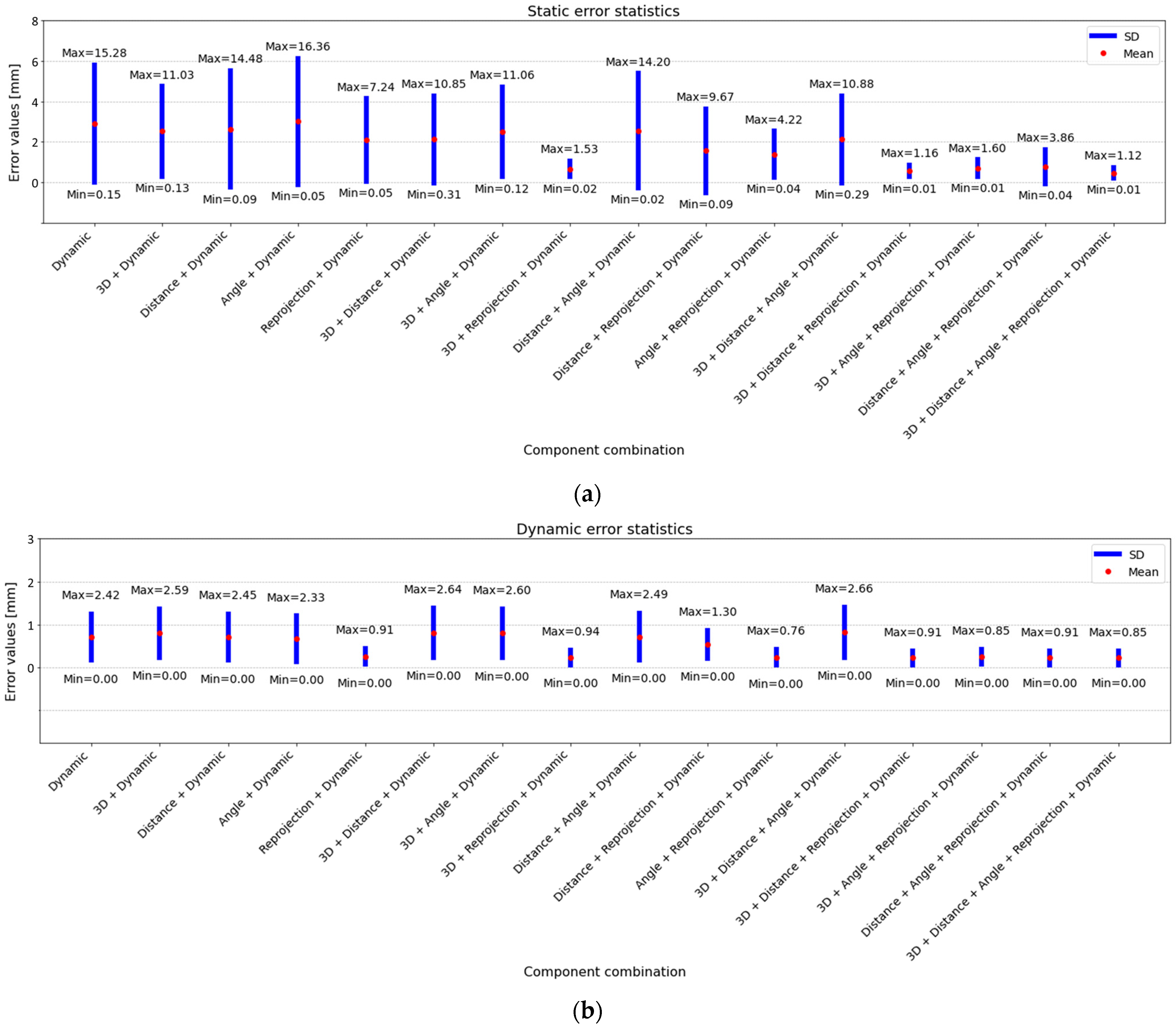
Sensitivity analysis was conducted to evaluate the influence of each error component in the proposed cost function on the final results, focusing on static error statistics, dynamic error statistics, and total error statistics. First, only static error components such as 3D coordinate errors, distance errors, angle errors, and reprojection errors, and their unique combinations without dynamic error components, were analyzed, and the results for static error statistics, dynamic error statistics, and total error statistics are shown in Figure S1. Then, all static error components, dynamic error components, and all their unique combinations were analyzed, and the results for static error statistics, dynamic error statistics, and total error statistics are shown in Figure 4.
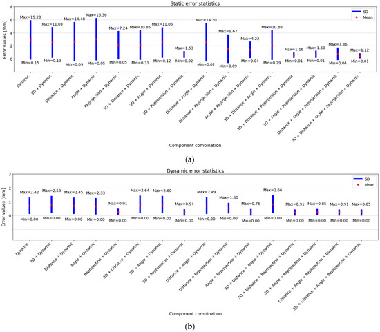
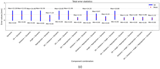
Figure 4.
Sensitivity analysis of static and dynamic error components of the proposed cost function. (a) Analysis of static errors based on 3D coordinates, distance, angle, and reprojection errors. (b) Dynamic error analysis based on the dynamic distance errors between wand markers. (c) Combined analysis of static and dynamic errors.
Among the static error components and their combinations, the combinations of 3D coordinate errors, distance errors and reprojection errors and of 3D coordinate errors, distance errors, angle errors, and reprojection errors produced the best results for static error statistics (Figure S1a). Both combinations resulted in a mean static error of 0.18 mm. However, 3D coordinate errors, distance errors, angle errors, and reprojection errors showed slightly better performance in terms of variability, with a standard deviation of 0.10 mm compared to 0.11 mm for 3D coordinate errors, distance errors, and reprojection errors. Additionally, 3D coordinate errors, distance errors, angle errors, and reprojection errors had a smaller minimum static error of 0.01 mm and a lower maximum static error of 0.41 mm, indicating more consistent accuracy across different test cases. While combinations such as distance errors and reprojection errors (mean: 0.23 mm, std: 0.16 mm) and distance errors and angle errors (mean: 0.32 mm, std: 0.27 mm) also showed relatively low static errors, 3D coordinate errors, distance errors, angle errors, and reprojection errors demonstrated the best overall performance in terms of both low mean error and low error spread.
When evaluating dynamic error statistics (Figure S1b), the best performance was achieved by the distance errors and angle errors combination, which produced a mean dynamic error of 2.12 mm, with a standard deviation of 1.53 mm and a maximum error of 5.34 mm. This was the lowest dynamic error among all combinations, suggesting that this combination effectively reduced discrepancies in wand distance measurements, which are critical for dynamic accuracy. However, the relatively high dynamic error across all other combinations, such as 3D coordinate errors, distance errors and reprojection errors and 3D coordinate errors, distance errors, angle errors and reprojection errors, highlights that static error components alone do not fully address dynamic tracking accuracy. To achieve more robustness and accuracy in tracking within the desired area outside the static frame, it is essential to incorporate dynamic error components into the cost function.
For total error statistics (Figure S1c), the distance errors and angle errors combination also yielded the best overall result, with a mean total error of 2.07 mm, a standard deviation of 1.54 mm, and a maximum error of 5.34 mm. This highlights the strength of this combination in balancing both static and dynamic error components. In contrast, while 3D coordinate errors, distance errors, and reprojection errors had lower static error, the higher dynamic error contributed to a higher total error of 2.60 mm. Similarly, 3D coordinate errors, distance errors, angle errors, and reprojection errors exhibited a total error of 2.61 mm, indicating that while these combinations excel in static error, they are less effective in achieving robust performance in dynamic error. For improved tracking accuracy across the entire target area, it is crucial to integrate dynamic error components into the optimization process.
Following the analysis of the static error components and their combinations, the next stage of the sensitivity analysis incorporates both static and dynamic error components. The inclusion of dynamic error components, such as wand distance errors, is crucial for improving tracking results across the desired area outside the static frame. The results for the sensitivity analysis, considering all static and dynamic error components and their unique combinations, are presented in Figure 4.
For the static error statistics (Figure 4a), the proposed cost function achieved the lowest mean static error of 0.46 mm with an SD of 0.26 mm, a minimum error of 0.01 mm, and a maximum error of 1.12 mm. This indicates that, although integrating both static and dynamic errors results in slightly higher static error compared to the optimal combinations in Figure 4 (which focused solely on static errors), the performance remains strong. By contrast, the cost function utilizing only reprojection errors [11,12] resulted in a mean static error of 2.10 mm, and the one using only 3D reconstruction errors [3] resulted in a mean static error of 2.52 mm. The integration of 3D coordinates and reprojection errors improved performance, with a mean static error of 0.66 mm. This demonstrates that while using individual error components like reprojection or 3D reconstruction alone can achieve some accuracy, integrating multiple error types significantly enhances calibration accuracy.
For dynamic error statistics (Figure 4b), the proposed cost function again demonstrated superior performance, recording a mean dynamic error of 0.23 mm, an SD of 0.16 mm, a minimum error of 0.00 mm, and a maximum error of 0.85 mm. The reprojection-only error component led to a mean dynamic error of 0.26 mm, while the 3D reconstruction-only component recorded a mean dynamic error of 0.80 mm. The combination of 3D coordinates and reprojection errors achieved a mean dynamic error of 0.24 mm. This consistency in reducing dynamic error across different static error combinations underscores the robustness of the proposed method.
For the total error statistics (Figure 4c), the proposed cost function achieved the lowest mean total error of 0.23 mm, an SD of 0.17 mm, a minimum error of 0.00 mm, and a maximum error of 1.12 mm, demonstrating the robustness of the proposed method. In contrast, the reprojection-only cost function resulted in a mean total error of 0.32 mm, while the 3D reconstruction-only cost function yielded a mean total error of 0.85 mm. The combination of 3D coordinates and reprojection errors resulted in a mean total error of 0.25 mm.
The sensitivity analysis reveals that while individual error components contribute to calibration accuracy, their combination in the proposed cost function results in superior performance. Specifically, 3D coordinate errors are crucial for accurate marker position reconstruction, but relying solely on them results in higher errors. Ensuring that distances between markers match known true distances is important, yet distance errors alone are inadequate. Maintaining geometric relationships between markers enhances structural integrity, although angle errors also need to be complemented by other error types. Directly minimizing discrepancies between observed and projected points significantly enhances accuracy, as demonstrated by the standalone reprojection error component. The best results were achieved when all static error components were combined with dynamic errors. This comprehensive approach ensures that all critical aspects of calibration accuracy are addressed, leading to the most accurate and robust calibration results. The proposed cost function, integrating 3D coordinate errors, distance errors, angle errors, and reprojection errors, significantly outperforms methods that use only reprojection or 3D reconstruction errors combined with dynamic errors. This underscores the importance of a holistic approach to error minimization in multi-camera calibration systems.
3.2. Comparative Analysis of the Proposed AIRLS Optimization Method
The performance of the proposed AIRLS optimization method was compared with those of advanced optimization techniques, specifically SBA and the LM method. The evaluation criteria included the average static error (encompassing 3D coordinates error, distance error, angle error), average dynamic error (wand distance error), and combined average error. All optimization methods were applied with default parameters and a tolerance of to terminate the optimization process. The results are summarized in Table 1.

Table 1.
Comparison of the proposed AIRLS optimization method with advanced optimization techniques.
The initial errors, before any optimization, exhibited an average static error of 0.36 mm, a dynamic error of 2.47 mm, and a total average error of 1.42 mm. Following the application of SBA optimization, the results indicated an average static error of 0.59 mm, a dynamic error of 0.25 mm, and a total average error of 0.42 mm. This method exhibited an SD of 0.35 mm for static error and 0.18 mm for dynamic error, with a minimum error of 0.10 mm and a maximum error of 1.26 mm for static error, and 0.00 mm and 0.96 mm for dynamic error, respectively. The LM optimization showed improvement, recording an average static error of 0.48 mm, a dynamic error of 0.23 mm, and a total average error of 0.36 mm. The SDs for static and dynamic errors were 0.28 mm and 0.15 mm, respectively. The minimum and maximum static errors measured 0.03 mm and 1.05 mm, respectively, while the dynamic errors ranged from 0.00 mm to 0.78 mm. The proposed AIRLS optimization method demonstrated superior performance compared to both SBA and LM techniques. The average static error was reduced to 0.28 mm, the dynamic error to 0.25 mm, and the total average error to 0.27 mm. The SD for the static error was 0.19 mm, and for the dynamic error, it was 0.25 mm. The minimum static error was 0.00 mm, with a maximum of 0.74 mm, and the dynamic errors ranged from 0.00 mm to 1.07 mm.
While other methods significantly reduced the dynamic error, they increased the static error. This indicates unbalanced optimization, with a bias towards minimizing dynamic error at the cost of static error accuracy, potentially leading to suboptimal camera parameters in a multi-camera system. Unlike these methods, the proposed AIRLS method effectively balances the optimization of both static and dynamic errors. This balanced approach ensures the simultaneous minimization of both types of errors, contributing to more accurate and robust optimization of the camera parameters. By iteratively adjusting the weights of the error components, the method prevents the dominance of either static or dynamic errors in the optimization process. This balanced and comprehensive approach consequently enhances the overall performance and accuracy of the multi-camera system.
The results clearly demonstrate that the proposed AIRLS optimization method surpassed other techniques in minimizing static and total errors, thereby achieving superior overall accuracy. The integration of the proposed cost function with the AIRLS method led to a substantial enhancement, especially in diminishing static error, which is crucial for precise multi-camera calibration. The inclusion and effective weighting of all static error components (3D coordinates, distances, angles, reprojection errors) in the optimization process were instrumental in this improved performance. Dynamic error remained relatively constant across all methods, indicating consistent wand distance measurements. Nevertheless, the proposed method’s balanced strategy in reducing both static and dynamic errors underscores its robustness in various calibration scenarios. The statistical analysis of errors, which includes average error, SD, minimum, and maximum values, further validates the precision and reliability of the AIRLS method for multi-camera calibration. Overall, the comparative analysis highlights the efficacy of the AIRLS optimization method in refining camera parameters, thus enhancing high-accuracy 3D reconstruction and tracking applications.
The analysis of the intrinsic, extrinsic, and distortion parameters for each camera in the multi-camera system, before and after optimization using AIRLS, shows marked improvements in calibration accuracy. Key parameters of each camera before and after optimization are concisely summarized in Table 2.
Table 2.
Camera parameters for each camera before and after optimization using AIRLS.
For Camera 1, the focal lengths and decreased slightly after optimization, indicating a refinement of the camera’s internal geometry. The skew parameter remained relatively constant, suggesting minimal corrections were needed for the angle between the image axes. The principal point coordinates and exhibited minor adjustments, likely correcting minor displacements from the image center. These adjustments in intrinsic parameters suggest more precise camera calibration, enhancing imaging accuracy. Camera 2 experienced an increase in the focal lengths and after optimization, which could be attributed to improved lens property estimations. The skew parameter increased slightly, indicating a minor adjustment in the angle between the image axes. The principal point coordinates and were adjusted to more accurately center the image. These changes reflect a more refined estimation of the intrinsic properties, resulting in improved calibration accuracy. For Camera 3, the focal lengths and exhibited minor changes, reflecting refined estimations of the intrinsic properties. The skew parameter decreased, correcting any angular deviations between the image axes. The principal point coordinates and were adjusted to correct the principal point offset. These adjustments indicate a precise calibration of the camera’s internal geometries. Camera 4 showed a decrease in the focal lengths and , indicating enhanced lens calibration accuracy. The skew parameter decreased slightly, suggesting a minor adjustment in the alignment of the image axes. The principal point coordinates and were significantly adjusted to correct the image center. These significant changes in intrinsic parameters post-optimization can be attributed to several factors. First, the initial camera parameters were computed using the normalized DLT method, which is known for its limitations in handling lens distortion and sensitivity to noise. DLT assumes a linear projection model and does not account for nonlinear distortions, leading to less accurate initial intrinsic estimates [17]. Additionally, the AIRLS method employed in the optimization process incorporates a combined cost function that accounts for both static and dynamic error components, along with regularization, which reduces overfitting and ensures a more robust parameter estimation. By refining these initial estimates through iterative optimization and integrating error minimization from multiple error sources, the camera’s intrinsic properties were corrected to reflect a more accurate and precise model of the internal camera geometry.
The extrinsic parameters also showed notable improvements. Camera 1′s rotation matrix and translation vector exhibited minor adjustments, indicating improved alignment of the camera’s orientation and position within the multi-camera setup. The minor adjustments to rotation angles and translation components suggest the fine-tuning of the camera’s spatial configuration. Camera 2 experienced significant changes in its rotation matrix and translation vector , indicating a considerable realignment of the camera’s orientation and position. This realignment could be attributed to the correction of the initial miscalibration post-optimization. Camera 3′s rotation matrix and translation vector displayed slight adjustments, reflecting minor corrections in the camera’s orientation and position. These changes suggest that the initial calibration was relatively accurate but required fine-tuning. Camera 4 exhibited significant modifications in its rotation matrix and translation vector , indicating substantial corrections to the camera’s spatial configuration. The likely correction of initial misalignments led to a more accurate overall setup. The alterations in extrinsic parameters across all cameras indicate that the optimization process effectively enhanced the spatial configuration of the multi-camera system, achieving improved alignment and positioning. The refinement of distortion coefficients across all cameras signifies that the lens distortion models were substantially improved, leading to enhanced image quality and diminished distortion artifacts. Specifically, Camera 1′s distortion coefficients underwent slight modifications, highlighting minor corrections in its lens distortion model. Camera 2 displayed substantial changes in its distortion coefficients, indicating major corrections in the lens distortion model. Adjustments in Camera 3′s distortion coefficients reflect enhancements in its lens distortion model, while significant alterations in Camera 4′s distortion coefficients point to major corrections in its lens distortion model.
Overall, the optimization process for camera parameters, as detailed in Table 2, clearly demonstrates that the proposed AIRLS method significantly enhances the accuracy of the intrinsic, extrinsic, and distortion parameters of the multi-camera system. The fine-tuning of intrinsic parameters augments the internal geometry of each camera, while adjustments in extrinsic parameters optimize spatial configuration and alignment. The refined distortion coefficients contribute to reduced lens distortions, thereby improving image quality.
In addition to the data presented in Table 2, further insights from the supplementary Table S1 allow for a deeper understanding of the optimization outcomes when comparing the AIRLS method with the LM approach. Table S1 highlights the intrinsic, extrinsic, and distortion parameter changes for each camera after optimization using both methods. The results from Table S1 reveal a consistent trend where both methods improve the calibration accuracy, but the AIRLS method generally provides finer adjustments, particularly in handling intrinsic parameters and minimizing lens distortion errors. This trend of more precise corrections extends across all cameras, where AIRLS offers a more controlled reduction in parameter deviations, particularly for the skew parameter and the principal point coordinates and , as demonstrated by smaller post-optimization adjustments in AIRLS.
Furthermore, the analysis of the five error components in the cost function (Equations (10)–(12), (14) and (15)) in Table S2 provides crucial insights into which aspects of the calibration process benefited the most from the AIRLS optimization. The results demonstrate that all error components showed improvements after optimization, with the most significant reduction observed in the dynamic wand distance error (Equation (15)). Initially averaging 2.47 mm, the dynamic error dropped dramatically to 0.25 mm post-optimization. This substantial reduction is vital, as it directly impacts the accuracy of dynamic calibration, enhancing the overall tracking performance across the target space. In terms of static errors, the 3D coordinate error (Equation (10)) experienced a marked improvement, decreasing from an average of 0.61 mm to 0.40 mm. This reduction underscores the AIRLS method’s efficacy in refining 3D reconstructions of marker positions. The reprojection error (Equation (14)) also saw significant improvement, with the error reduced from 0.16 mm to 0.12 mm, which reflects the better projection accuracy of 3D points onto the 2D image plane—an important factor for precise image-based tracking. The distance error (Equation (11)) and angle error (Equation (12)) showed more moderate but still notable improvements. The distance error decreased from 0.31 mm to 0.28 mm, while the angle error was reduced from 0.18 mm to 0.15 mm. These reductions contribute to better spatial relationships among the markers, further strengthening the calibration’s overall precision. The analysis confirms that while dynamic calibration experienced the greatest improvement, the reductions in 3D coordinate error and reprojection error also play crucial roles in enhancing static calibration accuracy. The comprehensive approach of the AIRLS method, which balances improvements across all error components, ensures a robust and reliable multi-camera calibration system that minimizes overfitting and delivers high-precision results.
The results in Table 3 offer a detailed comparison of the proposed multi-camera calibration method against the traditional normalized DLT and other related research methods. Each method underwent evaluation based on the average values from five trials, encompassing average error, SD, minimum error, and maximum error, with statistical significance determined using ANOVA and post-hoc tests.
Table 3.
Comparative analysis of multi-camera calibration techniques using 390 mm and 500 mm commercial calibration wands.
The proposed method demonstrated exceptional accuracy when validated using the 390 mm commercial calibration wand, achieving an average error of 0.42 ± 0.09 mm. This performance was significantly superior to the errors recorded for the normalized DLT (5.50 ± 1.80 mm), related research 1 (3.45 ± 0.15 mm), and related research 2 (1.21 ± 0.17 mm). The ANOVA results (F = 31.98, p = 0.00) confirm the statistical significance of these differences, indicating the superior accuracy of the proposed method.
Similarly, with the 500 mm commercial calibration wand, the proposed method recorded an average error of 0.46 ± 0.13 mm, surpassing the performance of the normalized DLT (6.73 ± 1.83 mm), related research 1 (3.77 ± 0.44 mm), and related research 2 (1.74 ± 0.07 mm). The ANOVA results (F = 42.01, p = 0.00) reinforce the statistical significance, underscoring the method’s robust performance across different validation tools.
Additionally, the analysis of SD across trials revealed that the proposed method not only achieved lower mean errors but also exhibited less variability in its measurements. For the 390 mm commercial calibration wand, the proposed method’s SD was 0.32 ± 0.10 mm, compared to the normalized DLT’s 3.02 ± 0.56 mm, related research 1′s 2.06 ± 0.15 mm, and related research 2′s 1.03 ± 0.23 mm. The 500 mm commercial calibration wand results mirrored this trend, with the proposed method exhibiting an SD of 0.43 ± 0.12 mm. This lower SD emphasizes the proposed method’s robustness and reliability, ensuring consistent results across different trials and conditions.
Minimum errors across all methods approached zero, demonstrating effective calibration capabilities. However, the proposed method consistently recorded significantly lower maximum errors (390 mm commercial calibration wand—1.48 ± 0.64 mm; 500 mm commercial calibration wand—1.82 ± 0.29 mm) compared to the normalized DLT and related research methods. This reflects the proposed method’s superior capability in handling outliers and extreme cases, offering a more stable and accurate calibration.
The discrepancy in errors between the validations using the 390 mm and 500 mm commercial calibration wands can likely be attributed to the varying distances between marker centers. The longer distance in the 500 mm commercial calibration wand likely led to a broader tracking zone, increasing the 3D triangulation error across all methods. Despite this, the increase in error for the proposed method was less pronounced, demonstrating its robustness in maintaining accuracy even within a broader tracking zone. This robustness is crucial as it suggests that the proposed method can adapt more effectively to varying calibration scenarios than the other methods.
The superior performance of the proposed method is attributed to its comprehensive cost function, which integrates multiple error components—3D coordinate, distance, angle, and reprojection errors for static errors, alongside dynamic wand distance error. This holistic approach significantly enhances the accuracy of calibration and 3D data triangulation by providing a more comprehensive assessment of potential discrepancies. Historically, simpler cost functions were often employed, which, while simpler to optimize, typically resulted in lower calibration accuracy. The complexity of this comprehensive cost function could potentially lead to an imbalance during the optimization process, wherein certain error components might dominate, causing inaccuracies. This challenge was effectively addressed by utilizing the AIRLS optimization method. AIRLS ensures balanced optimization by appropriately weighting both static and dynamic error components, preventing any single component from dominating the process. This balance mitigates the risk of overfitting or underfitting specific error types, thereby leading to more precise and robust calibration outcomes. The combination of the comprehensive cost function and the AIRLS optimization method represents a significant advancement in achieving precise multi-camera calibration.
Although the proposed method has its advantages, it shares some common limitations with other calibration techniques, such as the significant impact of input data quality on calibration accuracy. Errors may arise from poor marker detection or noise. Environmental factors, including lighting conditions and reflections, may also affect the precision of the calibration. Additionally, the method presupposes the rigidity of the calibration setup, which might not be consistent in all practical scenarios. Furthermore, the complexity of the proposed method, particularly due to the intricate cost function and AIRLS optimization, leads to longer computational time compared to other multi-camera calibration methods. While this additional time contributes to improved calibration accuracy by addressing key limitations in existing methods, it may be a concern in applications requiring faster performance or limited computational resources. Addressing this issue in future work could improve the method’s applicability across a wider range of resource-constrained settings. Additional research on regularization techniques and parameter correlation minimization would also be necessary to further enhance the robustness of the method. These limitations should be taken into account when implementing the proposed method across various environments and use cases.
4. Conclusions
This study introduces a novel multi-camera calibration method that merges static and dynamic calibration methods to improve accuracy and robustness. By integrating a comprehensive cost function with an AIRLS optimization method, the proposed technique adeptly balances static and dynamic error components, enabling precise 3D reconstruction and tracking. Extensive validation with 390 mm and 500 mm commercial calibration wands confirms that our method significantly outperforms traditional and other recently proposed methods. Despite some commonly shared limitations concerning data quality, environmental factors, and rigidity assumptions, the proposed method marks a notable advancement in multi-camera calibration, offering a dependable and efficient approach for complex calibration tasks. It provides a robust and efficient solution for high-precision applications across various fields, including optical motion capture, robotics, and surgical navigation systems.
Supplementary Materials
The following supporting information can be downloaded at https://www.mdpi.com/article/10.3390/photonics11090867/s1. Figure S1. Sensitivity analysis of static error components of the proposed cost function. (a) Analysis of static errors based on 3D coordinates, distance, angle, and reprojection errors. (b) Dynamic error analysis based on the dynamic distance errors between wand markers. (c) Combined analysis of static and dynamic errors; Table S1. Comparison of camera parameters before and after optimization using Levenberg-Marquardt (LM) and Adaptive Iter-atively Reweighted Least Squares (AIRLS) methods. Below each parameter in brackets, the difference from the parameter before optimization is indicated; Table S2. Comparison of initial and post-optimization errors for each cost function component using the proposed AIRLS method.
Author Contributions
Conceptualization, O.Y. and A.C.; methodology, O.Y.; validation, O.Y.; formal analysis, O.Y.; resources, Y.C. and J.H.M.; data curation, O.Y. and Y.C.; writing—original draft preparation, O.Y. and A.C.; writing—review and editing, O.Y. and A.C.; supervision, J.H.M.; project administration, J.H.M.; funding acquisition, J.H.M. All authors have read and agreed to the published version of the manuscript.
Funding
This research was funded by the Technology Innovation Program (project no: 20016285) funded by the Ministry of Trade, Industry and Energy (MOTIE, Korea).
Institutional Review Board Statement
Not applicable.
Informed Consent Statement
Not applicable.
Data Availability Statement
The data that support the findings of this study are available on request from the corresponding author. The data are not publicly available due to privacy or ethical restrictions.
Conflicts of Interest
The authors declare no conflicts of interest.
Abbreviations
| AIRLS | Adaptive iteratively reweighted least squares |
| DLT | Direct Linear Transformation |
| SBA | Sparse Bundle Adjustment |
| LM | Levenberg–Marquardt optimization method |
| P | Projection matrix |
| Intrinsic matrix | |
| R | Rotation matrix |
| T | Translation vector |
| F | Fundamental matrix |
| Focal lengths of the camera along the x and y axes | |
| Skew coefficient | |
| Principal point coordinates | |
| Rotation angles around the x, y, and z axes | |
| Translation vector along the x, y, and z axes | |
| Radial distortion coefficients | |
| Tangential distortion coefficients | |
| Static 3D coordinate error | |
| Static distance error | |
| Static angle error | |
| Static reprojection error | |
| Dynamic wand distance error |
References
- Wibowo, M.C.; Nugroho, S.; Wibowo, A. The use of motion capture technology in 3D animation. Int. J. Comput. Digit. Syst. 2024, 15, 975–987. [Google Scholar] [CrossRef] [PubMed]
- Yuhai, O.; Choi, A.; Cho, Y.; Kim, H.; Mun, J.H. Deep-Learning-Based Recovery of Missing Optical Marker Trajectories in 3D Motion Capture Systems. Bioengineering 2024, 11, 560. [Google Scholar] [CrossRef] [PubMed]
- Shin, K.Y.; Mun, J.H. A multi-camera calibration method using a 3-axis frame and wand. Int. J. Precis. Eng. Manuf. 2012, 13, 283–289. [Google Scholar] [CrossRef]
- Yoo, H.; Choi, A.; Mun, J.H. Acquisition of point cloud in CT image space to improve accuracy of surface registration: Application to neurosurgical navigation system. J. Mech. Sci. Technol. 2020, 34, 2667–2677. [Google Scholar] [CrossRef]
- Guan, J.; Deboeverie, F.; Slembrouck, M.; Van Haerenborgh, D.; Van Cauwelaert, D.; Veelaert, P.; Philips, W. Extrinsic Calibration of Camera Networks Using a Sphere. Sensors 2015, 15, 18985–19005. [Google Scholar] [CrossRef]
- Jiang, B.; Hu, L.; Xia, S. Probabilistic triangulation for uncalibrated multi-view 3D human pose estimation. In Proceedings of the 2023 IEEE/CVF International Conference on Computer Vision (ICCV), Paris, France, 1–6 October 2023; pp. 14850–14860. [Google Scholar] [CrossRef]
- Abdel-Aziz, Y.I.; Karara, H.M. Direct Linear Transformation from Comparator Coordinates into Object Space Coordinates in Close-Range Photogrammetry. Photogramm. Eng. Remote Sens. 2015, 81, 103–107. [Google Scholar] [CrossRef]
- Cohen, E.J.; Bravi, R.; Minciacchi, D. 3D reconstruction of human movement in a single projection by dynamic marker scaling. PLoS ONE 2017, 12, e0186443. [Google Scholar] [CrossRef]
- Mitchelson, J.; Hilton, A. Wand-Based Multiple Camera Studio Calibration. Center Vision, Speech and Signal Process Technical Report. Guildford, England. 2003. Available online: http://info.ee.surrey.ac.uk/CVSSP/Publications/papers/vssp-tr-2-2003.pdf (accessed on 8 May 2024).
- Pribanić, T.; Sturm, P.; Cifrek, M. Calibration of 3D kinematic systems using orthogonality constraints. Mach. Vis. Appl. 2007, 18, 367–381. [Google Scholar] [CrossRef]
- Petković, T.; Gasparini, S.; Pribanić, T. A note on geometric calibration of multiple cameras and projectors. In Proceedings of the 2020 43rd International Convention on Information, Communication and Electronic Technology (MIPRO), Opatija, Croatia, 28 September–2 October 2020; pp. 1157–1162. [Google Scholar] [CrossRef]
- Borghese, N.A.; Cerveri, P. Calibrating a video camera pair with a rigid bar. Pattern Recogn. 2000, 33, 81–95. [Google Scholar] [CrossRef]
- Uematsu, Y.; Teshima, T.; Saito, H.; Honghua, C. D-Calib: Calibration Software for Multiple Cameras System. In Proceedings of the 14th International Conference on Image Analysis and Processing, Modena, Italy, 10–14 September 2007; pp. 285–290. [Google Scholar] [CrossRef]
- Loaiza, M.E.; Raposo, A.B.; Gattass, M. Multi-camera calibration based on an invariant pattern. Comput. Graph. 2011, 35, 198–207. [Google Scholar] [CrossRef]
- Zhang, J.; Zhu, J.; Deng, H.; Chai, Z.; Ma, M.; Zhong, X. Multi-camera calibration method based on a multi-plane stereo target. Appl. Optics. 2019, 58, 9353–9359. [Google Scholar] [CrossRef] [PubMed]
- Zhou, C.; Tan, D.; Gao, H. A high-precision calibration and optimization method for stereo vision system. In Proceedings of the 2006 9th International Conference on Control, Automation, Robotics and Vision, Singapore, 5–8 December 2006; pp. 1–5. [Google Scholar] [CrossRef]
- Zhang, Z. A flexible new technique for camera calibration. IEEE Trans. Pattern Anal. Mach. Intell. 2000, 22, 1330–1334. [Google Scholar] [CrossRef]
- Pribanić, T.; Peharec, S.; Medved, V. A comparison between 2D plate calibration and wand calibration for 3D kinematic systems. Kinesiology 2009, 41, 147–155. [Google Scholar]
- Siddique, T.H.M.; Rehman, Y.; Rafiq, T.; Nisar, M.Z.; Ibrahim, M.S.; Usman, M. 3D object localization using 2D estimates for computer vision applications. In Proceedings of the 2021 Mohammad Ali Jinnah University International Conference on Computing (MAJICC), Karachi, Pakistan, 15–17 July 2021; pp. 1–6. [Google Scholar] [CrossRef]
- Lourakis, M.I.A.; Argyros, A.A. SBA: A software package for generic sparse bundle adjustment. ACM Trans. Math. Softw. (TOMS) 2009, 2, 1–30. [Google Scholar] [CrossRef]
- Nutta, T.; Sciacchitano, A.; Scarano, F. Wand-based calibration technique for 3D LPT. In Proceedings of the 2023 15th International Symposium on Particle Image Velocimetry (ISPIV), San Diego, CA, USA, 19–21 June 2023. [Google Scholar]
- Zheng, H.; Duan, F.; Li, T.; Li, J.; Niu, G.; Cheng, Z.; Li, X. A Stable, Efficient, and High-Precision Non-Coplanar Calibration Method: Applied for Multi-Camera-Based Stereo Vision Measurements. Sensors 2023, 23, 8466. [Google Scholar] [CrossRef]
- Zhang, S.; Fu, Q. Wand-Based Calibration of Unsynchronized Multiple Cameras for 3D Localization. Sensors 2024, 24, 284. [Google Scholar] [CrossRef]
- Hartley, R.I. In defense of the eight-point algorithm. IEEE Trans. Pattern Anal. Mach. Intell. 1997, 19, 580–593. [Google Scholar] [CrossRef]
- Fan, B.; Dai, Y.; Seo, Y.; He, M. A revisit of the normalized eight-point algorithm and a self-supervised deep solution. Vis. Intell. 2024, 2, 3. [Google Scholar] [CrossRef]
- Gonzalez, R.C.; Woods, R.E. Digital Image Processing, 4th ed.; Pearson Education: Rotherham, UK, 2002; ISBN 978-0-13-335672-4. [Google Scholar]
- Otsu, N. A Threshold Selection Method from Gray-Level Histograms. IEEE Trans. Syst. Man Cybern. 1979, 9, 62–66. [Google Scholar] [CrossRef]
- Suzuki, S.; Be, K. A Topological structural analysis of digitized binary images by border following. Comput. Vis. Graph. Image Process. 1985, 30, 32–46. [Google Scholar] [CrossRef]
- Kuhn, H.W. The Hungarian method for the assignment problem. Nav. Res. Logist. Q. 1955, 2, 83–97. [Google Scholar] [CrossRef]
- Troiano, M.; Nobile, E.; Mangini, F.; Mastrogiuseppe, M.; Conati Barbaro, C.; Frezza, F. A Comparative Analysis of the Bayesian Regularization and Levenberg-Marquardt Training Algorithms in Neural Networks for Small Datasets: A Metrics Prediction of Neolithic Laminar Artefacts. Information 2024, 15, 270. [Google Scholar] [CrossRef]
- Bellavia, S.; Gratton, S.; Riccietti, E. A Levenberg-Marquardt method for large nonlinear least-squares problems with dynamic accuracy in functions and gradients. Numer. Math. 2018, 140, 791–825. [Google Scholar] [CrossRef]
- Wang, T.; Karel, J.; Bonizzi, P.; Peeters, R.L.M. Influence of the Tikhonov Regularization Parameter on the Accuracy of the Inverse Problem in Electrocardiography. Sensors 2023, 23, 1841. [Google Scholar] [CrossRef]
- Silvatti, A.P.; Salve Dias, F.A.; Cerveri, P.; Barros, R.M. Comparison of different camera calibration approaches for underwater applications. J. Biomech. 2012, 45, 1112–1116. [Google Scholar] [CrossRef]

Disclaimer/Publisher’s Note: The statements, opinions and data contained in all publications are solely those of the individual author(s) and contributor(s) and not of MDPI and/or the editor(s). MDPI and/or the editor(s) disclaim responsibility for any injury to people or property resulting from any ideas, methods, instructions or products referred to in the content. |
© 2024 by the authors. Licensee MDPI, Basel, Switzerland. This article is an open access article distributed under the terms and conditions of the Creative Commons Attribution (CC BY) license (https://creativecommons.org/licenses/by/4.0/).