First Demonstration of Calibrated Color Imaging by the CAOS Camera

Abstract

The Coded Access Optical Sensor (CAOS) camera is a novel, single unit, full spectrum (UV to short-wave IR bands), linear, high dynamic range (HDR) camera. In this paper, calibrated color target imaging using the CAOS camera and a comparison to a commercial HDR CMOS camera is demonstrated for the first time. The first experiment using a calibrated color check chart indicates that although the CMOS sensor-based camera has an 87 dB manufacturer-specified HDR range, unrestricted usage of this CMOS camera’s output range greatly fails quality color recovery. On the other hand, the intrinsically linear full dynamic range operation CAOS camera color image recovery generally matches the restricted linear-mode commercial CMOS sensor-based camera recovery for the presented 39.5 dB non-HDR target that also matches the near 40 dB linear camera response function (CRF) range of the CMOS camera. Specifically, compared to the color checker chart manufacturer provided XYZ values for the calibrated target, percentage XYZ mean errors of 8.3% and 10.9% are achieved for the restricted linear range CMOS camera and CAOS camera, respectively. An alternate color camera assessment gives CIE ΔE₀₀ mean values of 4.59 and 5.7 for the restricted linear range CMOS camera and CAOS camera, respectively. Unlike the CMOS camera lens optics and its photo-detection electronics, no special linear response optics and photo-detector designs were used for the experimental CAOS camera, nevertheless, a good and equivalent color recovery was achieved. Given the limited HDR linear range capabilities of a CMOS camera and the intrinsically wide linear HDR capability of a CAOS camera, a combined CAOS-CMOS mode of the CAOS smart camera is prudent and can empower HDR color imaging. Applications for such a hybrid camera includes still photography imaging, especially for quantitative imaging of biological samples, valuable artworks and archaeological artefacts that require authentic color data generation for reliable medical decisions as well as forgery preventing verifications.

1. Introduction

There are many natural and human-made scenes with HDR near-continuous linear irradiance variation image content. To capture and display this linear HDR irradiance information, both linear HDR cameras as well as linear HDR displays are needed [1,2,3]. Specifically, to enable low contrast authentic target quantitative information detection embedded within these HDR scenes, it is critical that the camera have a linear camera response function (CRF) over the entire irradiance detection range. Recent results have shown that although classic silicon CMOS sensor-based cameras have excellent positive attributes for visible light operations such as high sensitivity, small pixel sizes, low power consumption, compact size, and large pixel counts [4], they can have a difficult time recovering low contrast (<6 dB step) targets within a linear HDR scene such as within a 90 dB range [5]. It is also known that both motion picture digital cinema production studios (e.g., use of 16 bits encoding for up-to 180 dB HDR scenes) [6] and display manufacturers (e.g., Apple Liquid Crystal HDR = 120 dB color display) [7] are looking to transition from classic 8-bit limited dynamic range sRGB or equivalent standard color images to 10 bits and higher color image generation and viewing to produce higher quality color scenes using a wider color gamut of the CIE 1931 XYZ color space. In fact, it is known that today’s color image capture and generation technologies do not have the capability to produce all perceivable colors called the human gamut in the CIE XYZ color space [8]. In addition, recent studies indicate that for HDR displays, conventional (gamma encoding) mapping “increasingly diverges from a perceptually uniform mapping, so 8-bit gray-levels are increasingly inadequate” [9]. Thus, it would be desirable to have an HDR linear response camera to enable the future potential for a near full human gamut color image capture and display. In addition, such a linear HDR camera if operating over a full spectrum from UV to short-wave IR (SWIR), i.e., 350 nm to 2600 nm can empower quantitative imaging of biological samples, precious artworks and archaeological artefacts that need authentic color data generation for accurate medical decisions and forgery prevention.

To provide an overall perspective on robust imager design using computational processing, early works using moving spatial masks such as via a spinning disk date back to 1949, when simultaneous capture of multiple optical wavelength channels using a single point photodetector was used to make a noise-robust infrared spectrometer [10,11]. Efforts to realize irradiance mappers using these spatial coding concepts evolved in the 1960s and 1970s [12,13,14,15]. In the late 1990s, with the emergence of the Texas Instruments (TI) digital micro-mirror device (DMD) as a highly programmable spatial mask generator, researchers proposed and demonstrated a variety of DMD-based imaging systems [16,17,18] including those based on the use of single point photodetectors for classical imaging [19,20] as well as compressive sensing imaging [21]. In particular, works popularly called “single pixel imaging” linked to the compressive camera described in [21] continue to evolve using the DMD to implement various compressive sensing algorithms for imaging [21,22,23,24].

Motivated by advances in the TI DMD technology with device pixel counts reaching 2 million micromirrors and micromirror temporal on-off modulation rates reaching 25 KHz with large (e.g., 170 × 1024 pixels) region-of-interest (ROI) frame rates of 50 KHz, proposed and demonstrated is a 177 dB HDR linear response [25] full spectrum capability high dynamic range camera called the coded access optical sensor or CAOS camera that is designed on the principles of the HDR RF mobile wireless cellular phone and data network. In the CAOS design, each pixel in the selected optical image space is treated like an independent cellular phone transmitting its unique data on a specific time-frequency RF code. Using the current DMD and the passive operational mode of the CAOS camera where the light source entering the camera aperture is temporally unmodulated, the unique CAOS RF frequency code assigned to a given pixel in the imaged irradiance can be designed to be as high as 25 KHz, providing ample temporal bandwidth for low noise high dynamic range photo-detection for the time-frequency image coded signal. With many (e.g., 4096) optical image RF coded data signals simultaneously detected by a few (e.g., 2) optical-to-RF antenna transducers, i.e., large area moderately high-speed point photodetectors, the time-frequency RF coded signals carrying all the harvested selected image pixel information are generated. Much like RF receivers in mobile phones, these RF signals from the point photodetectors are digitized and next undergo low noise filtering with time correlation signal processing and RF spectrum analysis using digital signal processing (DSP) techniques. These processing steps are used to recover the full optical spectrum image data over a linear HDR with signal-to-noise ratio (SNR) control for both pixel crosstalk reduction and HDR optimization. In effect, this single camera unit can simultaneously engage multiple spectral-band sensitive point detectors including using a DSLR-mode CMOS/CCD silicon sensor to form a full spectrum smart CAOS camera that can provide UV-SWIR imaging capabilities.

Most importantly, since the point photodetectors in the CAOS camera operate as linear response detectors with linear correlation and spectrum analysis signal processing low noise operations, a fundamentally linear camera with high linear dynamic range is possible. Given these capabilities with broadband optical spectrum operations, a hybrid CAOS-CMOS camera [26] for linear high dynamic range color imaging is a potential application where the linear dynamic range limitations (e.g., <60 dB) of the CMOS camera can be offset by the higher (i.e., >60 dB) linear dynamic range capabilities of the pixels-of-interest CAOS camera. In effect, the CMOS camera provides the fast access (e.g., 30 ms global frame time) high pixel count limited dynamic range color image while the CAOS camera recovers the much smaller pixel count (e.g., 1000) selective higher linear dynamic range pixel irradiances of the color image. CAOS image extraction time depends on the specific CAOS mode most effective for the given imaging scenario. Considering that the frequency modulated (FM) code division access multiplexed (CDMA) mode [25] of the CAOS camera is extracting 1024 CAOS pixels with an FM carrier rate of 25 KHz and 10 FM cycles allocated per CDMA bit, a (1024 × 10)/25 = 0.4096 s CAOS frame time is achieved. In other words, there is a tradeoff between the CAOS pixel count requiring high linear dynamic range access and the CAOS pixels frame recovery time. Hence, the hybrid CAOS-CMOS camera using the current DMD technology is suited for non-dynamic or slower speed applications such as high linear dynamic range color still photography.

Previously, basic uncalibrated CAOS white light color imaging was demonstrated without deploying camera color correction matrix and coordinate matrix transformations for color constancy and s-RGB format 8-bit displaying [27,28]. Given the potential of the CAOS camera for high quality quantitative color imaging including for human viewing, the present paper takes the first step towards this journey by designing and demonstrating the first calibrated white light color target CAOS imaging that engages color constancy matrix transformations. Furthermore, given the CAOS smart camera approach combines both CAOS and CMOS camera modes, the present paper also demonstrates CMOS-mode color imaging for comparison with CAOS color imaging. The rest of the paper provides details of these experiments and their data analysis highlighting the linear operation of the CAOS camera that is critical for linear HDR quantitative color imaging.

2. CMOS and CAOS Camera Color Imaging Testing Methods

Classic CMOS and CCD sensor cameras follow a specific signal processing chain when producing color images for human vision [29]. Consistent with prior camera testing methods, the methodology described next is deployed for testing both the CMOS camera and the CAOS camera. A 24 patch color checker calibrated TE 188 test chart model from Image Engineering (Kerpen, Germany) is chosen. This commercial vendor also provided the LG3 LED light source used in the experiments. The vendor uses a spectrophotometer to provide the CIE XYZ values for each patch of the TE 188 target using the LG3 5000 K illumination at 5000 lux. The following detailed steps are followed in the camera testing operations:

(1)

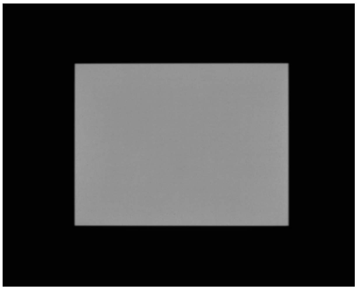
Use the camera under test to image the LG3 lightbox source illuminated test area without the transmissive color chart target placed in the lightbox. Confirm ≥ 95% spatial response uniformity of camera output over the white light screen test area given the LG3 lightbox is specified with a ≥95% spatial response uniformity over its illumination area. It has been pointed out earlier that camera spatial response uniformity is important for color imaging camera testing [30].

(2)

Using the TE 188 color checker chart placed at the LG3 lightbox illuminated test area, use the camera under test to take the three red (R), green (G), and blue (B) primary color images in time sequence using the selected Thorlabs (Newton, NJ, USA) R, G, B color filters models FD1R, FD1G, FD1B, respectively. The raw RGB pixel data is next averaged over its specific test patch area to provide averaged raw RGB data values R_raw, G_raw, and B_raw for the 24 test patches.

(3)

The test chart must include a white color patch that is needed for white balancing the raw RGB image data to introduce color constancy [31]. The averaged raw RGB data for the white patch is used to compute the camera raw RGB data weight balancing factors labelled as w_R = 1/[R_raw (white)], w_G = 1/[G_raw (white)], w_B = 1/[B_raw (white)]. For example, with camera provided white patch raw vector [R, G, B] = [5 7 9], the white balancing weights are w_R, = 1/5, w_G = 1/7, w_B =1/9. One implements the white balancing operation on the raw tri-simulus RGB data by using the formulas R_WB = w_R R_raw, G_WB = w_G G_raw, and B_WB = w_B B_raw.

(4)

Using the camera acquired RGB image data with the pre-calibrated CIE XYZ 3-D color space data provided by Image Engineering for the 24 patches of the TE-188 chart under LG3 illumination, next compute via an irradiance independent least squares regression optimization technique [32] the deployed camera color correction matrix that maps the camera white balanced RGB values to the CIE XYZ color space standard. The basics of the computation of the camera under test color correction matrix are as follows:

-

Let A represent the 3 × N matrix of experimentally acquired white balanced RGB (R_WB, G_WB, B_WB) camera outputs for N known color patches. Let B represent the 3 × N matrix of the known corresponding tristimulus X, Y, Z values provided by the commercial vendor using the measured spectral power distribution of the illuminant, the spectral function of each patch, and the CIE color matching functions. Using the known A and B matrices, compute the color correction matrix using the formula Φ = (AA^T)⁻¹.

-

Find the XYZ values for unknown (or new color patches) using the same illumination and deployed color filters for the test camera by deploying the computed 3 × 3 color correction Φ-matrix and using the following equation:

$$\left[\begin{array}{c}X\\ Y\\ Z\end{array}\right] = \left[\begin{array}{ccc}{\Phi }_{11}& {\Phi }_{12}& {\Phi }_{13}\\ {\Phi }_{21}& {\Phi }_{22}& {\Phi }_{23}\\ {\Phi }_{31}& {\Phi }_{32}& {\Phi }_{33}\end{array}\right]\left[\begin{array}{c}{R}_{WB} \\ G_{WB}\\ B_{WB}\end{array}\right]$$

For example, with the TE188 24 color patches chart, 23 colors are used to compute a Φ color correction matrix, and the one color left in the test chart is used as the test color transformed with the computed Φ matrix to generate the test color XYZ values. These experimentally determined XYZ values for this color are compared with the provided ground truth XYZ values provided by the commercial vendor for the deployed test color. Such a testing and comparison method is called leave-one-out cross-validation (LOOCV) [33] and its implementation using the TE188 24 color patches test chart is explained as follows:

LOOCV is a particular case of leave-p-out cross-validation with p = 1. LOOCV involves using one observation as the validation set and the remaining observations as the training set. This process is repeated for all observations, N and generates N test results. Given that the TE188 color checker target has 24 average RGB patch values, engaging LOOCV implies that one color from the chart is taken out and used for validation. This means that the other 23 colorss’ average RGB values and the corresponding X, Y, Z Image Engineering-provided ground truth values are used to find the color transformation matrix. Next one uses this specific Φ color correction matrix to find the X, Y, Z values for the left out one color, given its average RGB patch value provided by the test camera. Hence one can compare the camera provided X, Y, Z values with the ground truth X, Y, Z values for the left out one color. This color patch validation process one test color at a time is repeated for all 24 patches in the test camera viewed pre-calibrated color test chart. Completion of this process generates 24 XYZ values observed for all 24 colors of the TE 188 target seen by the test camera.

(5)

Both CIE XYZ and CIE L*a*b* are used for color camera performance analysis. First to assess visual observation via calibration error, Image Engineering-provided ground truth XYZ values are compared with the test camera measured XYZ values called X′, Y′, Z′ using the following root mean square (RMS) error and percentage error metrics [34]:

$$\begin{gathered} \mathrm{RMS} \mathrm{Error} = \sqrt{\frac{\Delta X^2+\Delta Y^2+\Delta Z^2}{3}} \\ \% \mathrm{Error} = 100\times \frac{\sqrt{\Delta X^2+\Delta Y^2+\Delta Z^2}}{\sqrt{X^2+Y^2+Z^2}} \end{gathered}$$

where ΔX = X − X′, ΔY = Y − Y′ and ΔZ = Z − Z′.

(6)

In addition, to calculate Delta E (CIE 2000) that is often considered for assessing the calibration error in terms of visual performance, we convert the XYZ values to L*a*b* values [35]. This conversion requires a reference white X_r, Y_r, Z_r which in our case is:

X_r = 95.047

Y_r = 100

Z_r = 108.833

$$\begin{gathered} \mathrm{L} = 116 f_y-16 \\ \mathrm{a} = 500 (f_x-f_y) \\ \mathrm{b} = 200 (f_y-f_z) \end{gathered}$$

where:

$$\begin{gathered} f_x = \{\begin{array}{c}\sqrt[3]{x_r} if x_r>ϵ \\ \frac{\kappa x_r+16}{116} otherwise\end{array} \\ {f}_y = \{\begin{array}{c}\sqrt[3]{y_r} if y_r>ϵ \\ \frac{\kappa y_r+16}{116} otherwise\end{array} \\ {f}_z = \{\begin{array}{c}\sqrt[3]{z_r} if y_r>ϵ \\ \frac{\kappa z_r+16}{116} otherwise\end{array} \\ {x}_r = \frac{X}{X_r} \\ {y}_r = \frac{Y}{Y_r} \\ {z}_r = \frac{Z}{Z_r} \\ ϵ = 0.008856 \\ \kappa = 903.3 \end{gathered}$$

Given Image Engineering-provided ground truth L*a*b* values and the test camera measured L*a*b* values, we calculate the ΔE₀₀ (CIE 2000) [36,37] which measures the difference or distance between two colors. A small value for ΔE₀₀ indicates that the colors are similar while a high value means that the colors are different.

(7)

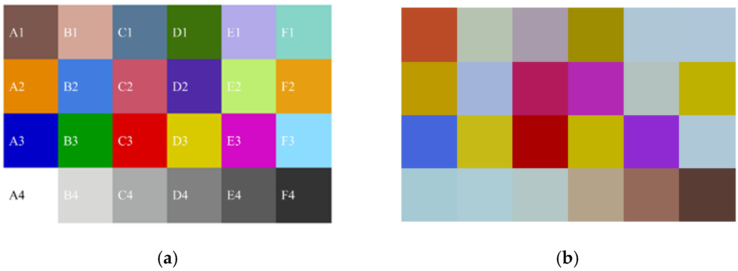
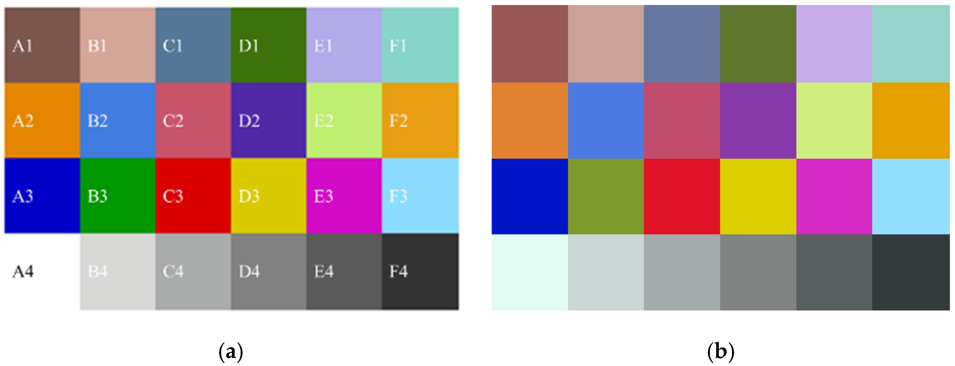
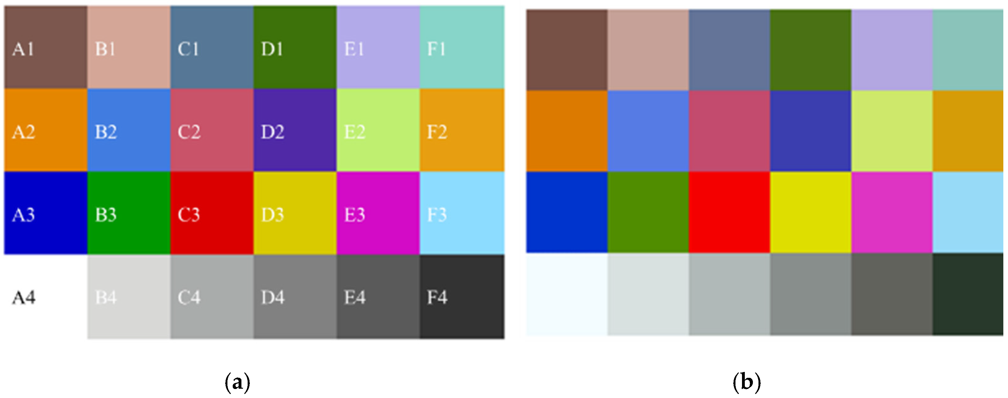
In order to visually observe both the Image Engineering-provided TE188 chart XYZ values and the test camera captured TE188 target 24 color patches on a standard 8-bit computer display, the following procedure is implemented [38]:

Find the chromaticity coordinates of an RGB system (x_R, y_R), (x_G, y_G) and (x_B, y_B) where:

x_R = X_R/(X_R + Y_R + Z_R); y_R = Y_R/(X_R + Y_R + Z_R)

x_G = X_G/(X_G + Y_G + Z_G); y_G = Y_G/(X_G + Y_G + Z_G)

x_B = X_B/(X_B + Y_B + Z_B); y_B = Y_B/(X_B + Y_B + Z_B)

Here X_R, Y_R, Z_R are the X, Y, and Z values of the red primary color patch, X_G, Y_G, Z_G are the X, Y, Z values of the green primary color patch, and X_B, Y_B, Z_B are the X, Y, Z values of the blue primary color patch. Given the XYZ values of the reference white patch for the LG3 light source as X_W, Y_W, Z_W, one can write:

$$\begin{gathered} {X^{\prime }}_R = x_R/(y_R {Z^{\prime }}_R) = (1 - x_R - y_R)/y_R \\ {X^{\prime }}_G = x_G/(y_G {Z^{\prime }}_G) = (1 - x_G - y_G)/y_G \\ {X^{\prime }}_B = x_B/(y_B {Z^{\prime }}_B) = (1 - x_B - y_B)/y_B \end{gathered}$$

Next, the following equations are used to find the RGB values for the test camera and Image Engineering-measured XYZ values:

$$\left[\begin{array}{c}{S}_R\\ S_G\\ S_B\end{array}\right] = {\left[\begin{array}{ccc}{X^{\prime }}_R& {X^{\prime }}_G& {X^{\prime }}_B\\ 1& 1& 1\\ {Z^{\prime }}_R& {Z^{\prime }}_G& {Z^{\prime }}_B\end{array}\right]}^{-1}\left[\begin{array}{c}{X}_W\\ X_W\\ X_W\end{array}\right] \mathrm{and} M = {\left[\begin{array}{ccc}{S}_R{X^{\prime }}_R& S_G{X^{\prime }}_G& S_B{X^{\prime }}_B\\ S_R& S_G& S_B\\ S_R{Z^{\prime }}_R& S_G{Z^{\prime }}_G& S_B{Z^{\prime }}_B\end{array}\right]}^{}$$

The computed M color coordinate matrix is used to find M⁻¹ and then used to find the measured linear RGB values for display operations via the equation given next:

$$\left[\begin{array}{c}{R}_{Linear}\\ G_{Linear}\\ B_{Linear}\end{array}\right] = M^{-1}\left[\begin{array}{c}X \\ Y\\ Z\end{array}\right]$$

(8)

Implemented is Gamma encoding and 8-bit scale conversion for the computed linear RGB values to display via the s-RGB standard on a commercial 8-bit color computer display. This operation is done using the following equations with a 2.4 gamma rating for the display [39]:

$$\begin{array}{c}if R_{Linear},G_{Linear},B_{Linear} \le 0.003031308 \\ R_{sRGB} = 12.92\times R_{Linear}\\ G_{sRGB} = 12.92\times G_{Linear}\\ B_{sRGB} = 12.92\times B_{Linear}\\ Otherwise if\\ R_{Linear},G_{Linear},B_{Linear}>0.003031308\\ R_{sRGB} \le 1.055\times {\left[R_{Linear}\right]}^{\left(1/2.4\right)}-0.055\\ G_{sRGB} \le 1.055\times {\left[G_{Linear}\right]}^{\left(1/2.4\right)}-0.055\\ B_{sRGB} \le 1.055\times {\left[B_{Linear}\right]}^{\left(1/2.4\right)}-0.055\end{array}$$

As the deployed color display is rated as a standard 8-bit display, the earlier equations provided R_sRGB, G_sRGB and B_sRGB values are multiplied by 255 and rounded off to nearest integer value to provide the final sRGB values that form the final 8-bit color images.

(9)

As the final step in the test camera pre-calibrated color imaging evaluation, in order to visually observe and compare the ground truth and test camera 24 color patches on standard 8-bit computer display, the final 8-bit s-RGB data for the two comparative images is fed to a display. One should note that for regular camera color imaging operations with unknown color scenes versus a comparative color checking operation using LOOCV with a known color checker, one deploys a single color correction matrix derived using a large (e.g., 140) set of known colors using Calibrite Digital ColorChecker SG [40] that can enable accurate and robust recovery of unknown colors on a per pixel basis [41].

3. CMOS Camera Color Imaging Experiment

The CMOS camera is set up in the laboratory to image the TE188 color chart under LG3 lightbox illumination. This camera uses a Thorlabs monochrome CMOS sensor model Quantalux S2100-M with 5.04 μm pixel pitch, 2.1 Mpixels and up-to an 87 dB HDR rating with a 16-bit (i.e., 0 to 65,535 levels) v_p output. The camera is fitted with a C-mount model GMZ18108 1.8 cm to 10.8 cm high quality multi-lens element color autofocus zoom lens that images the target screen illumination zone placed 234.7 cm from the sensor end of the camera. As the CMOS sensor size and target screen size are known, a demagnification factor of 95.75 is realized from target to sensor plane using the autofocus zoom lens. The LG3 illumination is set to 5000 lux and the CMOS camera with an exposure time of 4 ms is used to image the illumination screen without the color checker target. Figure 1 shows the captured CMOS camera image that confirms a high-quality spatial illumination uniformity of 96% given that the LG3 is specified with a ≥95% uniformity. In other words, pixel irradiance data analysis shows that 96% of the pixels in the CMOS camera imaged LG3 screen zone without placement of the color chart has the same irradiance values within a 0.25% irradiance fluctuation level set by the LG3 illumination controls. The lighter zone in Figure 1 is the illuminated LG3 screen zone where later the transmissive TE188 color target is placed for imaging. The average CMOS sensor output v_p(avg) is ~40,000 in a maximum 16-bit output keeping the CMOS sensor well under saturation for a robust spatial uniformity test.

The TE188 color checker chart is placed on the LG3 illumination screen and the CMOS camera takes the R, G, B images of the color target using a rotating color filter wheel fitted with the R, G and B optical filters. The HDR CMOS sensor exposure time is set to 50 ms as all three images brightest patches (i.e., the A4 white patch) are not saturating the 16-bit CMOS sensor output. Specifically, the highest CMOS pixel v_p value recorded is 46,801, indicating no saturated pixels in the three images. Unrestricted use of all the CMOS sensor 16-bit v_p outputs are deployed for the Section 2 described color image processing for 8-bit display.

Figure 2a shows the reconstructed 8-bit color images from the TE188 chart provided calibrated XYZ values for the 24 color patches while Figure 2b shows the reconstructed 8-bit color image using the unrestricted full 16-bit CMOS sensor output (i.e., v_p values ranging from 0 to 2¹⁶ − 1 = 65,535. When comparing with the actual ground truth patch colors shown in Figure 2a, the image in Figure 2b shows poor color recovery of the target patches. This poor recovery is due to the unrestricted use of the HDR CMOS v_p outputs in the 16-bit range. Recent experimental work with this specific CMOS sensor camera has shown an overall non-linear CRF over the 16-bit full range [5,41], hence one should expect a poor color recovery as proved by the current experiment. Earlier experiments for this CMOS sensor have also shown a highly improved linear response for CMOS sensor when maximum v_p output < 40,000 [5,42]. Clearly, linear CRF operations of a camera are vital to accurate color imaging. In order to demonstrate this point in the context of the experiments in this paper, the CMOS camera exposure time is reduced to 30 ms giving a restricted maximum v_p ≤ 38,045 regime. This v_p maximum restricted RGB data set is deployed to engage the linear region of the CMOS sensor’s CRF with

Table 1. Restricted linear CRF zone 16-bit CMOS sensor output usage CMOS camera color imaging experimental data table including patch averaged raw R, G, B Values and the TE188 chart provided calibrated XYZ values-based comparative error metrics data. CMOS sensor Exposure Time = 30 ms.

		Raw Values			Estimated			Real (Theoretical)
		R	G	B	X	Y	Z	X	Y	Z	RMS	%
A1	dark skin	1665.06	3690.63	1485.27	0.14	0.12	0.09	0.14	0.12	0.09	0.0022	1.91
B1	light skin	4498.57	14,979.84	5808.80	0.44	0.43	0.36	0.49	0.45	0.36	0.03	6.17
C1	blue sky	1208.35	6426.06	4931.85	0.17	0.17	0.29	0.15	0.17	0.30	0.01	6.38
D1	foliage	580.55	6437.22	367.16	0.10	0.14	0.04	0.07	0.12	0.04	0.02	20.69
E1	blue flower	4106.65	15,479.12	13,703.65	0.49	0.46	0.79	0.47	0.44	0.79	0.02	3.50
F1	bluish green	2074.91	23,971.33	10,455.57	0.43	0.56	0.64	0.41	0.55	0.64	0.01	2.72
A2	orange	5998.90	9353.95	833.50	0.44	0.34	0.06	0.46	0.36	0.07	0.02	4.54
B2	purplish blue	904.73	6560.23	11,425.79	0.20	0.19	0.64	0.21	0.20	0.69	0.03	7.22
C2	moderate red	4471.01	3337.52	2797.74	0.31	0.19	0.16	0.34	0.21	0.16	0.02	8.61
D2	purple	667.83	1459.02	6238.31	0.10	0.07	0.34	0.11	0.06	0.34	0.01	3.11
E2	yellow green	4142.87	30,837.50	3639.99	0.57	0.72	0.27	0.54	0.73	0.33	0.04	6.34
F2	orange yellow	6024.13	14,545.68	1355.44	0.49	0.45	0.11	0.50	0.44	0.10	0.01	3.03
A3	blue	151.93	518.05	9545.91	0.09	0.05	0.53	0.09	0.04	0.50	0.02	6.20
B3	green	556.26	9678.52	297.83	0.13	0.20	0.05	0.09	0.21	0.06	0.02	16.20
C3	red	6436.24	520.18	513.38	0.39	0.18	0.02	0.35	0.17	0.02	0.03	12.22
D3	yellow	4884.49	24,368.69	321.45	0.52	0.62	0.10	0.50	0.57	0.05	0.04	8.71
E3	magenta	6392.00	1251.79	9251.63	0.47	0.24	0.50	0.41	0.20	0.50	0.04	10.45
F3	cyan	2358.29	26,752.05	17,481.68	0.53	0.66	1.04	0.50	0.62	1.01	0.03	4.22
A4	white	7373.14	34,331.59	18,062.25	0.87	0.91	1.08	0.95	1.00	1.09	0.07	6.85
B4	neutral 65	5103.04	26,305.31	12,254.68	0.64	0.69	0.74	0.65	0.69	0.74	0.01	1.26
C4	neutral 39	3189.23	16,336.23	7453.54	0.40	0.43	0.45	0.38	0.41	0.44	0.02	4.28
D4	neutral 21	1817.73	9042.79	4101.63	0.22	0.24	0.25	0.21	0.22	0.24	0.01	6.65
E4	neutral 10	992.74	4331.11	2038.16	0.11	0.12	0.12	0.10	0.10	0.11	0.01	14.29
F4	neutral 3	401.19	1495.90	815.89	0.04	0.04	0.05	0.03	0.03	0.04	0.01	33.74
		RMSE					Percentage Difference
		Mean	Median	95%	Max		Mean	Median	95%	Max
		0.022	0.018	0.041	0.069		8.30	6.36	20.02	20.69

and

Table 2. Restricted linear CRF zone 16-bit CMOS sensor output usage CMOS camera color imaging experimental data table including patch averaged raw R, G, B Values and the TE188 chart provided calibrated L*a*b* values-based comparative error metrics data. CMOS sensor Exposure Time = 30 ms.

Patch	Camera Measured RGB Values			Camera Measured			Lab Image Engg. Reference
	R	G	B	L	a	b	L	a	b	∆E00
A1	1665.06	3690.63	1485.27	41.43	17.94	11.92	41.23	16.55	11.79	0.96
B1	4498.57	14,979.84	5808.80	71.64	10.04	13.25	72.58	18.37	14.17	6.49
C1	1208.35	6426.06	4931.85	48.87	1.66	−16.45	48.39	−7.26	−19.36	8.36
D1	580.55	6437.22	367.16	44.63	−27.03	38.38	41.93	−37.07	35.23	5.71
E1	4106.65	15,479.12	13,703.65	73.69	15.19	−25.10	72.11	14.68	−27.82	1.90
F1	2074.91	23,971.33	10,455.57	79.69	−28.11	−2.94	79.21	−32.76	−2.98	2.04
A2	5998.90	9353.95	833.50	65.08	36.26	62.15	66.36	36.53	61.82	1.07
B2	904.73	6560.23	11,425.79	50.72	11.18	−52.14	52.18	6.59	−54.09	3.55
C2	4471.01	3337.52	2797.74	50.77	55.33	10.54	53.38	54.42	14.97	3.49
D2	667.83	1459.02	6238.31	31.43	31.93	−54.49	29.46	45.42	−57.34	6.15
E2	4142.87	30,837.50	3639.99	88.09	−27.94	53.33	88.56	−35.82	46.06	5.27
F2	6024.13	14,545.68	1355.44	72.93	18.74	59.67	71.97	23.75	62.02	2.81
A3	151.93	518.05	9545.91	26.47	42.63	−83.80	22.95	61.04	−86.92	8.20
B3	556.26	9678.52	297.83	52.36	−38.49	48.66	53.39	−67.75	42.32	10.73
C3	6436.24	520.18	513.38	50.09	87.03	62.97	48.76	77.63	58.60	2.45
D3	4884.49	24,368.69	321.45	82.84	−17.45	81.20	80.20	−10.32	92.36	5.28
E3	6392.00	1251.79	9251.63	55.90	85.78	−29.91	51.94	85.25	−37.50	4.56
F3	2358.29	26,752.05	17,481.68	84.75	−21.67	−23.46	83.03	−22.34	−24.48	1.25
A4	7373.14	34,331.59	18,062.25	96.35	1.75	−5.78	100.00	0.00	0.00	5.94
B4	5103.04	26,305.31	12,254.68	86.64	−4.87	0.82	86.33	−0.41	0.43	5.70
C4	3189.23	16,336.23	7453.54	71.62	−3.88	1.68	69.85	−0.29	−0.13	5.15
D4	1817.73	9042.79	4101.63	56.03	−2.34	1.79	54.04	−0.28	0.00	3.76
E4	992.74	4331.11	2038.16	40.91	1.35	1.35	38.27	−0.22	−0.15	3.53
F4	401.19	1495.90	815.89	24.55	4.24	−1.04	21.14	0.22	−0.61	5.79
	∆E
	Mean	Median	0.95	Max
	4.59	4.85	8.34	10.73

and Figure 3 showing the XYZ values, L*a*b* values, and recovered color image, respectively.

As expected, compared to the Figure 2b recovered color image using the unrestricted full 16-bit HDR CMOS sensor output data that uses a nonlinear CRF, the Figure 3b color image with restricted CMOS sensor data processing using only smaller but linear zone of the CRF creates a greatly improved color image when compared to the ground truth image. This experiment also shows that although many CMOS cameras may be specified as HDR cameras, their high-quality color image recovery is restricted to a non-HDR zone as achieving continuous linear photo-pixel operation over a HDR range is highly limited due to various factors that include silicon CMOS array sensor device fabrication physics limits to optoelectronic and electronic circuit readout signal noise issues.

4. CAOS Camera Color Imaging Experiment

The CAOS camera design shown in Figure 4 is implemented in the laboratory using the following key components: National Instruments (Austin, TX, USA) 16-bit Analog-to-Digital Converter (ADC) model 6366, LG3 5000 K Lightbox, Vialux (Chemnitz, Germany) DMD model V-700, DELL (Round Rock, TX, USA) Latitude model 5480 laptop for control and DSP, and Thorlabs components that include model PDA100A2 silicon point photo-detectors (PDs) set at 40 dB electronic gain, 1.62 cm diameter Iris A1, 5.08 cm diameter 10 cm focal length front imaging lens L1, 5.08 cm diameter spherical mirrors SM1 and SM2 with 3.81 cm focal lengths, and 2.54 cm diameter FD1 model RGB color filters within the F1 filter wheel. The inter-component distances are: L1: DMD of 10.4 cm; SM1/SM2:DMD of 9.8 cm; SM1/SM2:PD1/PD2 of 6.3 cm and target:L1 of 265 cm. A factor of 25.5 demagnification takes place between target plane and DMD plane and a demagnification factor of 1.56 between the DMD and PD1/PD2 planes.

The basics of the CAOS camera operations are as follows: Light from the target is imaged on to the DMD plane using lens L1 that is a basic visible light spherical lens. The on/off binary tilt state micromirrors in the DMD are programmed in the CAOS code-division multiple access (CDMA)-imaged light time-frequency encoding mode such that each CAOS pixel on the DMD has its unique 4096-bits Walsh time sequence code [25]. The encoded image zone on the DMD consists of 4060 = 70 × 58 CAOS pixels with each CAOS pixel containing 13 × 13 micromirrors. Each micromirror is 13.68 μm × 13.68 μm size. The first experimental step for the CAOS camera is to conduct the camera spatial uniformity check by imaging the white light screen on LG3 without placing the TE188 target. This is done without using any color filter inside the F1 color filter wheel. A 1 KHz CDMA bit rate is used for an ADC rate of 1 Msps with the LG3 illumination at 65.8 Klux. The recovered CAOS camera image is shown in Figure 5 using a color bar for irradiance normalized gray-scaling with a mean scaled irradiance of 0.76. Irradiance data analysis from the CAOS camera Figure 5 image for the LG3 white screen indicates a 95% uniformity suited for TE188 color chart imaging. In other words, pixel irradiance data analysis shows that 95% of the pixels in the CAOS camera imaged LG3 screen zone without placement of the color chart has the same irradiance values within a 0.25% (i.e., 1/4000) irradiance fluctuation level set by the LG3 illumination controls.

Next, the TE188 color chart is imaged by the CAOS camera with the F1 color filter wheel containing the R, G, B filters and CAOS encoding using a 16 KHz CDMA bit rate with an ADC rate of 1.6 Msps with the LG3 illumination at 39.5 Klux.

Table 3. CAOS camera color imaging experimental data table including patch averaged raw R, G, B values and the TE188 chart provided calibrated XYZ values-based comparative error metrics data.

	Raw Values			Estimated			Real (Theoretical)
	R	G	B	X	Y	Z	X	Y	Z	RMS	%
A1	0.173	0.078	0.064	0.12	0.11	0.08	0.14	0.12	0.09	0.01	11.82
B1	0.519	0.327	0.298	0.43	0.40	0.35	0.49	0.45	0.36	0.04	9.83
C1	0.114	0.149	0.270	0.16	0.17	0.31	0.15	0.17	0.30	0.01	3.79
D1	0.041	0.151	0.016	0.09	0.13	0.04	0.07	0.12	0.04	0.01	10.93
E1	0.428	0.339	0.660	0.46	0.43	0.73	0.47	0.44	0.79	0.03	5.76
F1	0.191	0.485	0.444	0.37	0.47	0.54	0.41	0.55	0.64	0.08	14.54
A2	0.693	0.206	0.039	0.41	0.31	0.05	0.46	0.36	0.07	0.04	12.13
B2	0.100	0.157	0.649	0.23	0.21	0.71	0.21	0.20	0.69	0.02	4.84
C2	0.545	0.080	0.161	0.31	0.19	0.16	0.34	0.21	0.16	0.02	7.52
D2	0.062	0.031	0.352	0.10	0.07	0.38	0.11	0.06	0.34	0.02	10.83
E2	0.463	0.742	0.190	0.57	0.72	0.31	0.54	0.73	0.33	0.02	3.88
F2	0.630	0.318	0.054	0.43	0.39	0.09	0.50	0.44	0.10	0.05	12.17
A3	0.014	0.010	0.492	0.10	0.06	0.52	0.09	0.04	0.50	0.02	6.69
B3	0.033	0.238	0.011	0.12	0.20	0.05	0.09	0.21	0.06	0.02	12.41
C3	0.845	0.008	0.021	0.43	0.19	−0.02	0.35	0.17	0.02	0.06	24.69
D3	0.598	0.638	0.009	0.57	0.68	0.12	0.50	0.57	0.05	0.08	18.65
E3	0.735	0.034	0.495	0.46	0.24	0.50	0.41	0.20	0.50	0.04	8.99
F3	0.237	0.606	0.823	0.51	0.62	0.95	0.50	0.62	1.01	0.03	4.60
A4	0.817	0.870	0.910	0.89	0.96	1.08	0.95	1.00	1.09	0.04	4.15
B4	0.603	0.654	0.671	0.68	0.73	0.81	0.65	0.69	0.74	0.05	7.09
C4	0.380	0.428	0.430	0.44	0.47	0.52	0.38	0.41	0.44	0.07	16.07
D4	0.214	0.241	0.234	0.24	0.26	0.28	0.21	0.22	0.24	0.04	18.12
E4	0.107	0.108	0.101	0.11	0.12	0.12	0.10	0.10	0.11	0.02	14.46
F4	0.016	0.035	0.022	0.03	0.03	0.03	0.03	0.03	0.04	0.01	17.28
	RMSE					Percentage Difference
	Mean	Median	95%	Max		Mean	Median	95%	Max
	0.034	0.034	0.077	0.082		10.88	10.88	18.57	24.69

shows the CAOS camera provided experimental data along with the Image Engineering provided calibrated XYZ values-based comparative error metrics data. In addition,

Table 4. CAOS camera color imaging experimental data table including patch averaged raw R, G, B values and the TE188 chart provided calibrated L*a*b* values-based comparative error metrics data.

Patch	Camera Measured RGB Values			Camera Measured			Camera Measured RGB Values
	R	G	B	L	a	b	L	a	b	∆E00
A1	0.173	0.078	0.064	38.95	17.14	12.65	41.23	16.55	11.79	2.09
B1	0.519	0.327	0.298	69.59	14.44	10.27	72.58	18.37	14.17	3.84
C1	0.114	0.149	0.270	48.34	0.60	−20.29	48.39	−7.26	−19.36	7.27
D1	0.041	0.151	0.016	43.29	−31.34	34.64	41.93	−37.07	35.23	2.63
E1	0.428	0.339	0.660	71.27	15.12	−24.92	72.11	14.68	−27.82	1.66
F1	0.191	0.485	0.444	74.10	−24.40	−2.71	79.21	−32.76	−2.98	5.26
A2	0.693	0.206	0.039	62.54	38.88	64.91	66.36	36.53	61.82	3.30
B2	0.100	0.157	0.649	52.96	14.20	−54.92	52.18	6.59	−54.09	4.88
C2	0.545	0.080	0.161	51.04	56.33	9.02	53.38	54.42	14.97	3.96
D2	0.062	0.031	0.352	32.12	30.87	−57.53	29.46	45.42	−57.34	7.91
E2	0.463	0.742	0.190	87.86	−26.02	47.85	88.56	−35.82	46.06	4.80
F2	0.630	0.318	0.054	68.96	17.36	59.98	71.97	23.75	62.02	4.28
A3	0.014	0.010	0.492	29.03	39.16	−79.11	22.95	61.04	−86.92	9.37
B3	0.033	0.238	0.011	52.06	−43.03	44.93	53.39	−67.75	42.32	8.33
C3	0.845	0.008	0.021	51.06	94.49	118.79	48.76	77.63	58.60	15.94
D3	0.598	0.638	0.009	85.98	−18.20	80.88	80.20	−10.32	92.36	6.62
E3	0.735	0.034	0.495	56.19	80.58	−30.03	51.94	85.25	−37.50	4.68
F3	0.237	0.606	0.823	82.88	−19.65	−20.89	83.03	−22.34	−24.48	1.90
A4	0.817	0.870	0.910	98.28	−2.97	−2.58	100.00	0.00	0.00	4.72
B4	0.603	0.654	0.671	88.40	−3.29	−1.26	86.33	−0.41	0.43	4.36
C4	0.380	0.428	0.430	74.39	−4.13	−0.43	69.85	−0.29	−0.13	6.08
D4	0.214	0.241	0.234	58.43	−3.54	0.83	54.04	−0.28	0.00	5.99
E4	0.107	0.108	0.101	41.28	−0.89	2.39	38.27	−0.22	−0.15	3.69
F4	0.016	0.035	0.022	21.62	−11.48	5.61	21.14	0.22	−0.61	13.35
	∆E
	Mean	Median	95%	Max
	5.70416	4.75777	12.7495	15.9409

shows the CAOS camera color imaging experimental data table including patch averaged raw R, G, B values and the TE188 chart provided calibrated L*a*b* values-based comparative error metrics data.

XYZ mean error of 10.9 is achieved for the CAOS camera. The alternate color camera assessment gives ΔE₀₀ mean value of 5.7 for the CAOS camera.

Figure 6 shows the reconstructed 8-bit color images from the Image Engineering-provided calibrated XYZ values for the 24 color patches versus the CAOS camera-captured image. Review of Table 3 and Table 4 and Figure 6 indicates a color patch recovery of the presented 39.5 dB dynamic range color checker target to be similarly good quality in performance to the restricted CMOS camera mode recovery. In particular, these comparisons indicate the robustness of the intrinsically linear operation CAOS camera that allows unrestricted usage of its output that is highly desirable when operating with HDR color targets. Given the CAOS smart camera design engages both the CMOS and CAOS modes of the camera system, a combined CAOS-CMOS mode would combine the best attributes of CMOS and CAOS. One should note that none of the lens and mirror optics as well as the large area silicon point detectors and electronics in the CAOS camera assembly were optimized for linear and uniform gain operations over the visible color band. On the contrary, the commercial CMOS camera uses a high quality commercial multi-element zoom lens designed for color imaging. These aspects can be linked to the slight mismatch in color imaging performance metrics for the restricted range CMOS camera and the unrestricted range CAOS camera.

5. Conclusions

Presented is the first experimental proof-of-concept color imaging CAOS camera. For first stage comparison studies with the CAOS camera, a commercial CMOS-sensor based camera with a monochrome CMOS sensor specified with up-to an 87 dB dynamic range is tested in the laboratory. R, G, B color filters deployed time-sequentially provide raw RGB image data via the two cameras under test. The experiments use a commercial imaging test house LG3 LED white light 5000 K spectrum source that illuminates a calibrated 24 color patches target with a 39.5 dB maximum instantaneous dynamic range that matches the restricted linear CRF region of the CMOS camera. After raw RGB data white balancing and camera color correction matrix computations for the two cameras for color constancy processing, CIE standard XYZ values are computed for the observed target. Compared to the TE188 chart provided XYZ values for the calibrated target, percentage XYZ mean errors of 8.3% and 10.9% are achieved for the restricted linear range CMOS camera and the unrestricted range CAOS camera, respectively. An alternate color camera assessment gives ΔE₀₀ mean values of 4.59 and 5.7 for the restricted linear range CMOS camera and unrestricted range CAOS camera, respectively.

For visual display on a standard computer display, the four different experimental XYZ data are used to produce comparative 8-bit color images for the 24-patch target using XYZ to sRGB LG3 source color coordinate matrix-based conversion with gamma encoding. Results indicate that although the CMOS sensor has an HDR range, unrestricted usage of sensor output fails color recovery and the intrinsically linear operation unrestricted range CAOS camera color image recovery generally matches the restricted linear-mode commercial CMOS sensor-based camera recovery for the presented non-HDR target. It is to be noted that unlike the CMOS camera lens optics and its photo-detection electronics, no special linear response optics and photo-detector designs were used for the CAOS camera experiment. Nevertheless, an equivalent color recovery was achieved indicating that given the limited HDR linear range capabilities of a CMOS camera and the intrinsically wide linear HDR capability of a CAOS camera, a combined hybrid CAOS-CMOS mode is an optimal approach to achieve linear HDR color imaging. Hence, the CAOS smart camera that combines CAOS and CMOS modes can empower high quality HDR color imaging such as for HDR color still photography. Future work relates to using a calibrated HDR color target with a linearity optimized CAOS camera design for color imaging tests and deployment of this CAOS camera for testing of HDR colored human-made [43] and natural scenes.

References

1. McCann, J.J.; Rizzi, A. The Art and Science of HDR Imaging; John Wiley & Sons: Hoboken, NJ, USA, 2012. [Google Scholar]
2. Reinhard, E.; Ward, G.; Pattanaik, S.; Debevec, P. High Dynamic Range Imaging: Acquisition, Display, and Image-Based Lighting; Elsevier Morgan Kaufmann Publisher: Burlington, MA, USA, 2005. [Google Scholar]
3. Banterle, F.; Artusi, A.; Debattista, K.; Chalmers, A. Advanced High Dynamic Range Imaging—Theory and Practice; CRC Press, Taylor & Francis Group: Oxfordshire, UK, 2011. [Google Scholar]
4. Gouveia, L.C.P.; Choubey, B. Advances on CMOS image sensors. Sens. Rev. 2016, 36, 231–239. [Google Scholar] [CrossRef] [Green Version]
5. Riza, N.A.; Mazhar, M.A. Robust Low Contrast Image Recovery over 90 dB Scene Linear Dynamic Range using CAOS Camera. In Proceedings of the IS & T Electronic Imaging; Society for Imaging Science and Technology: Burlingame, CA, USA, 2020; pp. 1–10. [Google Scholar]
6. Academy of Motion Picture Arts and Sciences (AMPAS). S-2008–001. Academy Color Encoding Specification (ACES) Version 1.0; Academy of Motion Picture Arts and Sciences: Los Angeles, CA, USA, 2008. [Google Scholar]
7. Apple. Pro Display XDR. Available online: https://www.apple.com/ie/pro-display-xdr (accessed on 20 February 2021).
8. Hoffmann, G. CIE Color Space; Technical Report; University of Applied Sciences: Emden, Germany, 2000. [Google Scholar]
9. Vargas, A.; Johnson, P.; Kim, J.; Hoffman, D. A perceptually uniform tone curve for OLED and other high dynamic range displays. J. Vis. 2014, 14, 83. [Google Scholar] [CrossRef]
10. Golay, M.J.E. Multi-Slit Spectrometry. J. Opt. Soc. Am. 1949, 39, 437–444. [Google Scholar] [CrossRef]
11. Fellgett, P.I. —les principes généraux des méthodes nouvelles en spectroscopie interférentielle-A propos de la théorie du spectromètre interférentiel multiplex. J. Phys. Radium 1958, 19, 187–191. [Google Scholar] [CrossRef] [Green Version]
12. Gottlieb, P. A television scanning scheme for a detector-noise limited system. IEEE Trans. Inform. Theory 1968, 14, 428–433. [Google Scholar] [CrossRef]
13. Ibbett, R.N.; Aspinall, D.; Grainger, J.F. Real-Time Multiplexing of Dispersed Spectra in Any Wavelength Region. Appl. Opt. 1968, 7, 1089–1093. [Google Scholar] [CrossRef]
14. Decker, J.A., Jr.; Harwitt, M.O. Sequential Encoding with Multislit Spectrometers. Appl. Opt. 1968, 7, 2205–2209. [Google Scholar] [CrossRef]
15. Decker, J.A., Jr. Hadamard-Transform Image Scanning. Appl. Opt. 1970, 9, 1392–1395. [Google Scholar] [CrossRef]
16. Kearney, K.; Ninkov, Z. Characterization of a digital micro-mirror device for use as an optical mask in imaging and spectroscopy. Proc. SPIE 1998, 3292, 81–92. [Google Scholar]
17. Castracane, J.; Gutin, M. DMD-based bloom control for intensified imaging systems. Proc. SPIE 1999, 3633, 234–242. [Google Scholar]
18. Nayar, S.; Branzoi, V.; Boult, T. Programmable imaging using a digital micro-mirror array. Proc. IEEE Conf. Comput. Vis. Pattern Recognit. 2004, 1, 436–443. [Google Scholar]
19. Sumriddetchkajorn, S.; Riza, N.A. Micro-electro-mechanical system-based digitally controlled optical beam profiler. Appl. Opt. 2002, 41, 3506–3510. [Google Scholar] [CrossRef]
20. Riza, N.A.; Mughal, M.J. Optical power independent optical beam profiler. Opt. Eng. 2004, 43, 793–797. [Google Scholar] [CrossRef]
21. Takhar, D.; Laska, J.N.; Wakin, M.; Duarte, M.; Baron, D.; Sarvotham, S.; Kelly, K.; Baraniuk, R.G. A new compressive imaging camera architecture using optical-domain compression. Proc. SPIE 2006, 6065, 606509. [Google Scholar] [CrossRef]
22. Durán, V.; Clemente, P.; Fernández-Alonso, M.; Tajahuerce, E.; Lancis, J. Single-pixel polarimetric imaging. Opt. Lett. 2012, 37, 824–826. [Google Scholar] [CrossRef] [PubMed] [Green Version]
23. Shin, J.; Bosworth, B.T.; Foster, M.A. Single-pixel imaging using compressed sensing and wavelength-dependent scattering. Opt. Lett. 2016, 41, 886–889. [Google Scholar] [CrossRef]
24. Zhang, Z.; Liu, S.; Peng, J.; Yao, M.; Zheng, G.; Zhong, J. Simultaneous spatial, spectral, and 3D compressive imaging via efficient Fourier single-pixel measurements. Optica 2018, 5, 315–319. [Google Scholar] [CrossRef]
25. Riza, N.A.; Mazhar, M.A. 177 dB Linear Dynamic Range Pixels of Interest DSLR CAOS Camera. IEEE Photonics J. 2019, 11, 1–10. [Google Scholar] [CrossRef]
26. Riza, N.A.; La Torre, J.P.; Amin, M.J. CAOS-CMOS camera. Opt. Express 2016, 24, 13444–13458. [Google Scholar] [CrossRef]
27. Riza, N.A.; Mazhar, M.A. Demonstration of CAOS Smart Camera Imaging for Color and Super Blue Moon Targets. In Proceedings of the OSA Advanced Photonics Congress on Sensors, Zurich, Switzerland, 2–5 July 2018. paper SeW2E.3. [Google Scholar]
28. Riza, N.A.; Mazhar, M.A.; Ashraf, N. Solar Limb Darkening Color Imaging of the Sun with the Extreme Brightness Capability CAOS Camera. In London Imaging Meeting; Society for Imaging Science and Technology: London, UK, 2020; Volume 2020, pp. 69–73. [Google Scholar]
29. Ramantha, R.; Snyder, W.E.; Yoo, Y.; Drew, M.S. Color Image Processing Pipeline: A general survey of digital still cameras. IEEE Signal Process. Mag. 2005, 22, 34–43. [Google Scholar] [CrossRef]
30. Pointer, M.R.; Attridge, G.G.; Jacobson, R.E. Practical camera characterization for colour measurement. Imaging Sci. J. 2001, 49, 63–80. [Google Scholar] [CrossRef]
31. Ebner, M. Color Constancy; Kriss, M.A., Ed.; Wiley-IS&T Series in IS&T; Wiley: Hoboken, NJ, USA, 2007. [Google Scholar]
32. Bastani, P.; Funt, B. Simplifying irradiance independent color calibration. Proc. SPIE 2014, 9015, 90150N. [Google Scholar]
33. Celisse, A. Optimal cross-validation in density estimation with the L2-loss. Ann. Stat. 2014, 42, 1879–1910. [Google Scholar] [CrossRef]
34. Hyndman, R.; Koehler, A.B. Another look at measures of forecast accuracy. Int. J. Forecast. 2006, 22, 679–688. [Google Scholar] [CrossRef] [Green Version]
35. Lindblom, B. XYZ to Lab. Available online: http://www.brucelindbloom.com/index.html?Eqn_XYZ_to_Lab.html (accessed on 15 January 2021).
36. Fraser, B.; Murphy, C.; Bunting, F. Real World Color Management; Peachpit Press: San Francisco, CA, USA, 2004. [Google Scholar]
37. Lindblom, B. Delta E (CIE 2000 B). Available online: http://www.brucelindbloom.com/index.html?Eqn_DeltaE_CIE2000.htm (accessed on 15 January 2021).
38. Lindblom, B. RGB/XYZ Matrices. Available online: http://www.brucelindbloom.com/Eqn_RGB_XYZ_Matrix.html (accessed on 15 January 2021).
39. IEC 61966-2-1:1999. IEC Webstore; International Electrotechnical Commission: Geneva, Switzerland, 1999. [Google Scholar]
40. Imatest LLC. Calibrite Digital ColorChecker SG. Available online: https://store.imatest.com/test-charts/color-charts/colorchecker-sg.html (accessed on 15 January 2021).
41. Imatest LLC. Color Correction Matrix. Available online: http://www.imatest.com/docs/colormatrix (accessed on 15 January 2021).
42. Riza, N.A.; Ashraf, N. Calibration Empowered Minimalistic MultiExposure Image Processing Technique for Camera Linear Dynamic Range Extension. In Proceedings of the IS & T Elect. Imaging Conference; Society for Imaging Science and Technology: Burlingame, CA, USA, 2020; pp. 2131–2136. [Google Scholar]
43. Riza, N.A.; Mazhar, M.A. Robust Testing of Displays using the Extreme Linear Dynamic Range CAOS Camera. In Proceedings of the 2019 IEEE 2nd British and Irish Conference on Optics and Photonics (BICOP), London, UK, 11–13 December 2019. [Google Scholar]
Figure 1. CMOS camera image of the illumination screen to confirm a camera spatial response uniformity of 96% desirable for camera color imaging testing.
Photonics 08 00538 g001
Figure 2. Reconstructed 8-bit color images from (a) TE188 chart provided calibrated XYZ values for the 24 color patches and (b) Un-Restricted Full 16-bit CMOS Sensor Output Usage CMOS camera operations engaging a nonlinear CRF.
Photonics 08 00538 g002
Figure 3. Reconstructed 8-bit color images from (a) Image Engineering provided calibrated XYZ values for the 24 color patches and (b) Restricted 16-bit CMOS Sensor Output Usage CMOS camera linear CRF operations.
Photonics 08 00538 g003
Figure 4. Basic CAOS camera design implemented in the laboratory.
Photonics 08 00538 g004
Figure 5. CAOS camera image of the illumination screen to confirm a camera spatial response uniformity of 95% desirable for camera color imaging testing.
Photonics 08 00538 g005
Figure 6. Reconstructed 8-bit color images from (a) TE188 chart provided calibrated XYZ values for the 24 color patches and (b) CAOS camera.
Photonics 08 00538 g006