Laser Self-Mixing Sensor for Simultaneous Measurement of Young’s Modulus and Internal Friction


Abstract
:1. Introduction
2. Measurement Principle
2.1. The Equations for Young’s Modulus and Internal Friction
2.2. The Sensing Principle of SMI
3. Results
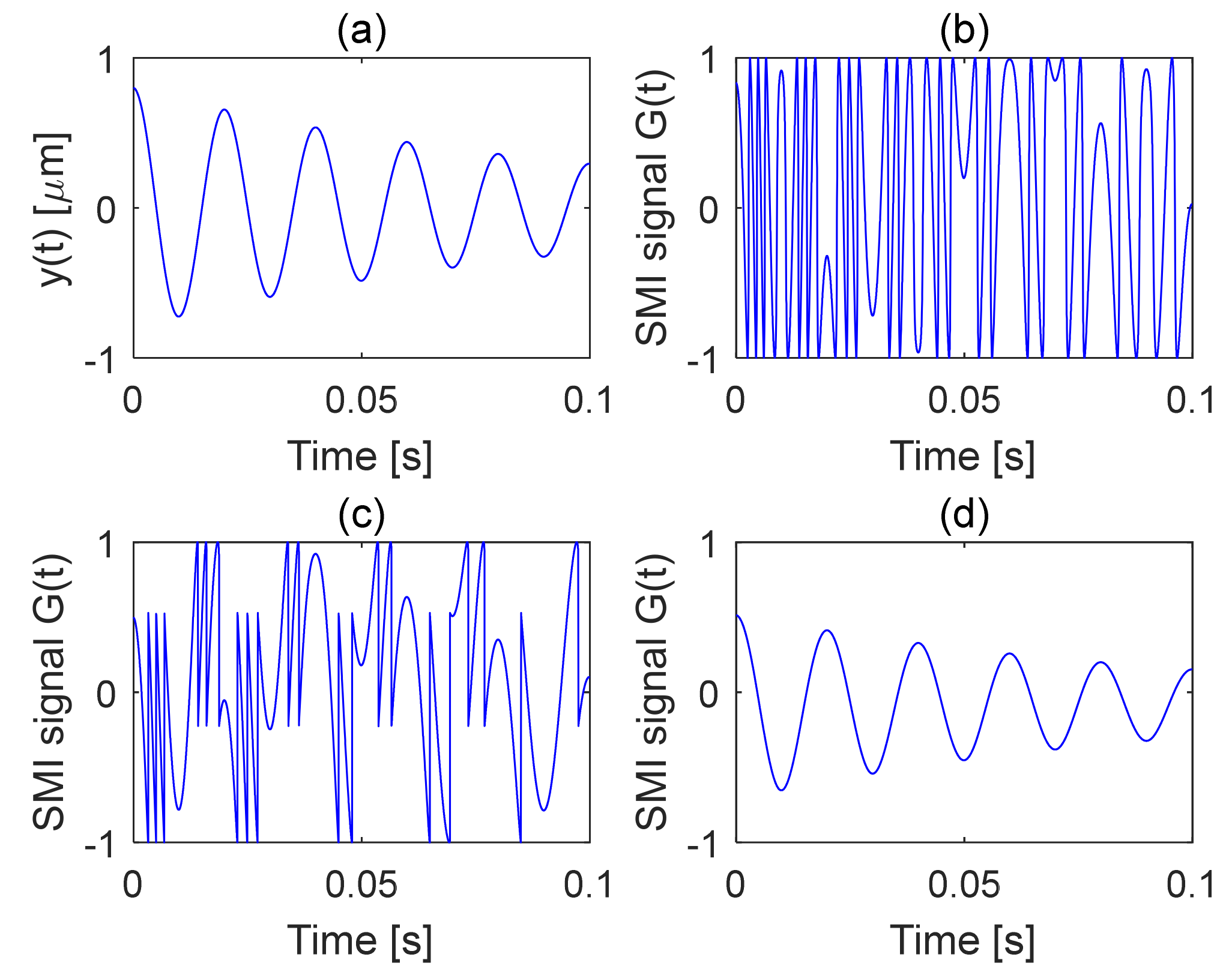
3.1. Simulation
3.2. Experiment
4. Discussion
5. Conclusions
Author Contributions
Funding
Institutional Review Board Statement
Informed Consent Statement
Data Availability Statement
Conflicts of Interest
References
- Roebben, G.; Bollen, B.; Brebels, A.; Van Humbeeck, J.; Van der Biest, O. Impulse excitation apparatus to measure resonant frequencies, elastic moduli, and internal friction at room and high temperature. Rev. Sci. Instrum. 1997, 68, 4511–4515. [Google Scholar] [CrossRef]
- Xie, M.; Ding, G.; Jiang, M.; Li, F. High-frequency elastic moduli and internal frictions of Zr41.2Ti13.8Cu12.5Ni10Be22.5 bulk metallic glass during glass transition and crystallization. J. Non-Cryst. Solids 2021, 560, 120754. [Google Scholar] [CrossRef]
- Lord, J.D.; Morrell, R.M. Elastic modulus measurement—Obtaining reliable data from the tensile test. Metrologia 2010, 47, S41–S49. [Google Scholar] [CrossRef]
- Shetty, D.K.; Rosenfield, A.R.; McGuire, P.; Bansal, G.K.; Duckworth, W.H. Biaxial flexure tests for ceramics. Am. Ceram. Soc. Bull. 1980, 59, 1193–1197. [Google Scholar]
- Suansuwan, N.; Swain, M.V. Determination of elastic properties of metal alloys and dental porcelains. J. Oral Rehabil. 2001, 28, 133–139. [Google Scholar] [CrossRef] [PubMed]
- Schmidt, R.; Alpern, P.; Tilgner, R. Measurement of the Young’s modulus of moulding compounds at elevated temperatures with a resonance method. Polym. Test. 2005, 24, 137–143. [Google Scholar] [CrossRef]
- Lin, K.; Yu, Y.; Xi, J.; Li, H.; Guo, Q.; Tong, J.; Su, L. A Fiber-Coupled Self-Mixing Laser Diode for the Measurement of Young’s Modulus. Sensors 2016, 16, 928. [Google Scholar] [CrossRef] [Green Version]
- Xia, F.; Liu, B.; Cao, L.; Yu, Y.; Xi, J.; Guo, Q.; Tong, J. Experimental study on simultaneously measuring Young’s modulus and internal fraction using self-mixing system. In Semiconductor Lasers and Applications VIII, (International Society for Optics and Photonics; SPIE: Beijing, China, 2018; p. 1081212. [Google Scholar]
- Taimre, T.; Nikolić, M.; Bertling, K.; Lim, Y.L.; Bosch, T.; Rakić, A.D. Laser feedback interferometry: A tutorial on the self-mixing effect for coherent sensing. Adv. Opt. Photonics 2015, 7, 570–631. [Google Scholar] [CrossRef]
- Amin, S.; Zabit, U.; Bernal, O.D.; Hussain, T. High Resolution Laser Self-Mixing Displacement Sensor under Large Variation in Optical Feedback and Speckle. IEEE Sens. J. 2020, 20, 9140–9147. [Google Scholar] [CrossRef]
- Guo, D.; Shi, L.; Yu, Y.; Xia, W.; Wang, M. Micro-displacement reconstruction using a laser self-mixing grating interferometer with multiple-diffraction. Opt. Express 2017, 25, 31394–31406. [Google Scholar] [CrossRef] [Green Version]
- Zhu, D.; Zhao, Y.; Tu, Y.; Li, H.; Xu, L.; Yu, B.; Lu, L. All-fiber laser feedback interferometer using a DBR fiber laser for effective sub-picometer displacement measurement. Opt. Lett. 2021, 46, 114–117. [Google Scholar] [CrossRef]
- Guo, D.; Wang, M. Self-mixing interferometry based on a double-modulation technique for absolute distance measurement. Appl. Opt. 2007, 46, 1486–1491. [Google Scholar] [CrossRef]
- Norgia, M.; Melchionni, D.; Pesatori, A. Self-mixing instrument for simultaneous distance and speed measurement. Opt. Lasers Eng. 2017, 99, 31–38. [Google Scholar] [CrossRef]
- Zhao, Y.; Wang, C.; Zhao, Y.; Zhu, D.; Lu, L. An All-Fiber Self-Mixing Range Finder with Tunable Fiber Ring Cavity Laser Source. J. Light. Technol. 2021, 39, 4217–4224. [Google Scholar] [CrossRef]
- Chen, J.; Zhu, H.; Xia, W.; Guo, D.; Hao, H.; Wang, M. Self-mixing birefringent dual-frequency laser Doppler velocimeter. Opt. Express 2017, 25, 560–572. [Google Scholar] [CrossRef] [PubMed]
- Zhang, X.; Gu, W.; Jiang, C.; Gao, B.; Chen, P. Velocity measurement based on multiple self-mixing interference. Appl. Opt. 2017, 56, 6709–6713. [Google Scholar] [CrossRef]
- Usman, M.; Zabit, U.; Bernal, O.D.; Raja, G.; Bosch, T. Detection of Multimodal Fringes for Self-Mixing-Based Vibration Measurement. IEEE Trans. Instrum. Meas. 2019, 69, 258–267. [Google Scholar] [CrossRef]
- Zabit, U.; Bony, F.; Bosch, T.; Rakić, A.D. A Self-Mixing Displacement Sensor with Fringe-Loss Compensation for Harmonic Vibrations. IEEE Photonics Technol. Lett. 2010, 22, 410–412. [Google Scholar] [CrossRef]
- Wang, C.; Fan, X.; Guo, Y.; Gui, H.; Wang, H.; Liu, J.; Yu, B.; Lu, L. Full-circle range and microradian resolution angle measurement using the orthogonal mirror self-mixing interferometry. Opt. Express 2018, 26, 10371–10381. [Google Scholar] [CrossRef] [PubMed]
- Zhao, Y.; Fan, X.; Wang, C.; Lu, L. An improved intersection feedback micro-radian angle-measurement system based on the Laser self-mixing interferometry. Opt. Lasers Eng. 2020, 126, 105866. [Google Scholar] [CrossRef]
- Annovazzi-Lodi, V.; Merlo, S.; Norgia, M. Measurements on a micromachined silicon gyroscope by feedback interferometry. IEEE/ASME Trans. Mechatron. 2001, 6, 1–6. [Google Scholar] [CrossRef]
- Yu, Y.; Xi, J.; Chicharo, J.F. Measuring the feedback parameter of a semiconductor laser with external optical feedback. Opt. Express 2011, 19, 9582–9593. [Google Scholar] [CrossRef] [PubMed] [Green Version]
- El Assad, J.; Bosch, T.; Plantier, G. Laser Diode Under Strong Feedback for Mechatronics Applications. In Proceedings of the SENSORS, 2007 IEEE, Atlanta, GA, USA, 28–31 October 2007; pp. 387–390. [Google Scholar]
- Liu, B.; Ruan, Y.; Yu, Y. All-Fiber Laser-Self-Mixing Sensor for Acoustic Emission Measurement. J. Light. Technol. 2021, 39, 4062–4068. [Google Scholar] [CrossRef]
- ASTM. ASTM E1876 01, Standard Test Method for Dynamic Young’s Modulus, Shear Modulus, and Poisson’s Ratio by Impulse Excitation of Vibration; ASTM International: West Conshohocken, PA, USA, 2005; Available online: https://www.astm.org/Standards/E1876.htm (accessed on 11 February 2005).
- Donati, S.; Giuliani, G.; Merlo, S. Laser diode feedback interferometer for measurement of displacements without ambiguity. IEEE J. Quantum Electron. 1995, 31, 113–119. [Google Scholar] [CrossRef]
- Yu, Y.; Xi, J.; Chicharo, J.F.; Bosch, T.M. Optical Feedback Self-Mixing Interferometry with a Large Feedback Factor C: Behavior Studies. IEEE J. Quantum Electron. 2009, 45, 840–848. [Google Scholar] [CrossRef]
- Liu, B.; Ruan, Y.; Yu, Y.; Xi, J.; Guo, Q.; Tong, J.; Rajan, G. Laser Self-Mixing Fiber Bragg Grating Sensor for Acoustic Emission Measurement. Sensors 2018, 18, 1956. [Google Scholar] [CrossRef] [Green Version]
- Donati, S. Developing self-mixing interferometry for instrumentation and measurements. Laser Photonics Rev. 2012, 6, 393–417. [Google Scholar] [CrossRef]


| Specimen | Brass | Aluminum | |||
|---|---|---|---|---|---|
| Parameters | Average Value | Standard Deviation | Average Value | Standard Deviation | |
| Resonant frequency fRO | 453 Hz | 0.50 Hz | 596 Hz | 0.60 Hz | |
| Damping factor k | |||||
| Young’s modulus E | 117.9 GPa | 0.20 GPa | 69.4 GPa | 0.14 GPa | |
| Internal friction | 0.00080 | 0.00174 | |||
Publisher’s Note: MDPI stays neutral with regard to jurisdictional claims in published maps and institutional affiliations. |
© 2021 by the authors. Licensee MDPI, Basel, Switzerland. This article is an open access article distributed under the terms and conditions of the Creative Commons Attribution (CC BY) license (https://creativecommons.org/licenses/by/4.0/).
Share and Cite
Wang, B.; Liu, B.; An, L.; Tang, P.; Ji, H.; Mao, Y. Laser Self-Mixing Sensor for Simultaneous Measurement of Young’s Modulus and Internal Friction. Photonics 2021, 8, 550. https://doi.org/10.3390/photonics8120550
Wang B, Liu B, An L, Tang P, Ji H, Mao Y. Laser Self-Mixing Sensor for Simultaneous Measurement of Young’s Modulus and Internal Friction. Photonics. 2021; 8(12):550. https://doi.org/10.3390/photonics8120550
Chicago/Turabian StyleWang, Bo, Bin Liu, Lei An, Pinghua Tang, Haining Ji, and Yuliang Mao. 2021. "Laser Self-Mixing Sensor for Simultaneous Measurement of Young’s Modulus and Internal Friction" Photonics 8, no. 12: 550. https://doi.org/10.3390/photonics8120550