Three-Dimensional Laser Imaging with a Variable Scanning Spot and Scanning Trajectory

Abstract

Traditional lidar scans the target with a fixed-size scanning spot and scanning trajectory. Therefore, it can only obtain the depth image with the same pixels as the number of scanning points. In order to obtain a high-resolution depth image with a few scanning points, we propose a scanning and depth image reconstruction method with a variable scanning spot and scanning trajectory. Based on the range information and the proportion of the area of each target (PAET) contained in the multi echoes, the region with multi echoes (RME) is selected and a new scanning trajectory and smaller scanning spot are used to obtain a finer depth image. According to the range and PAET obtained by scanning, the RME is segmented and filled to realize the super-resolution reconstruction of the depth image. By using this method, the experiments of two overlapped plates in space are carried out. By scanning the target with only forty-three points, the super-resolution depth image of the target with 160 × 160 pixels is obtained. Compared with the real depth image of the target, the accuracy of area representation (AOAR) and structural similarity (SSIM) of the reconstructed depth image is 99.89% and 98.94%, respectively. The method proposed in this paper can effectively reduce the number of scanning points and improve the scanning efficiency of the three-dimensional laser imaging system.

1. Introduction

Three-dimensional (3D) imaging lidar obtains the intensity and distance information of the target at the same time [1,2]. According to different working modes, 3D imaging lidar can be categorized into two types, scanning and non-scanning. Scanning imaging lidar works by scanning the targets point by point with a small scanning spot [3,4]. In contrast, non-scanning imaging lidar needs large detector arrays because of the large laser spot. Therefore, a laser source with a large diameter and a high power leads to the bulky volume of the system [5,6]. However, the production and manufacture of large detector arrays are relatively difficult [7,8], and the use of a high-power laser increases the manufacturing cost. Compared with non-scanning mode, the scanning mode has the advantages of low laser energy and manufacturing costs [9,10]. Therefore, it is widely used in automatic driving [11,12], mapping [13], 3D image measurement [14], remote sensing [15,16] and environmental monitoring [17,18,19].

No matter whether the scanning mode is mechanical scanning [20,21] or non-mechanical scanning [22,23,24], the location of the scanning spot needs to be changed gradually to cover the whole field of view. The commonly used scanning methods include progressive scanning [25], circular scanning [26], and retina-like scanning [27,28]. These traditional scanning methods use a fixed-size scanning spot to scan the whole field of view (FOV) in a fixed trajectory. This kind of scanning method needs to ensure the number of scanning points consistent with the number of pixels of the reconstructed depth image. However, the interested region is usually smaller than the background region in the FOV. It increases the number of unnecessary scanning points and reduces the scanning efficiency, when scanning the interested region and the background region with the scanning points of the same density. Therefore, these traditional scanning methods are difficult to obtain high-resolution depth image with high scanning efficiency by using the scanning points of the same density to scan the whole FOV. Aimed at addressing this problem, Ling Ye et al. proposed an adaptive target profile acquiring method, and this method uses the depth hop of adjacent pixels based on photon counting to determine the depth boundaries of targets [29]. However, this method cannot accurately judge the region of multi-target by comparing the depth hop of adjacent pixels. At the same time, it uses bicubic interpolation to reconstruct the super-resolution depth image. This method does not consider the real reflection area of the target, so the reconstructed super-resolution depth image using this method is not accurate.

Therefore, we propose a scanning and depth image reconstruction method with the variable scanning spot and scanning trajectory. Based on the intensity and range contained in the multi echoes generated by different targets in a single scanning, the range of each target and PAET are obtained from the multi echoes. Firstly, a large scanning spot is used to scan the target to obtain the location information of the sub-region with multi-target and the PAET. After that, the scanning spot is reduced, and a new scanning trajectory is planned to scan sub-regions to obtain more precise information of targets. Then according to the location and PAET obtained by scanning, the RME is segmented and filled to realize the super-resolution reconstruction of the depth image. Compared with traditional scanning methods, the proposed method can significantly reduce the number of scanning points and obtain high-resolution depth images.

In this paper, the model of the reflection area and range of each target in multi echoes is established. Then, the scanning strategy of the variable scanning spot and scanning trajectory and the depth image restoration method are established. In the laboratory test, the target is scanned by a large-scale scanning spot to obtain RMEs, and the reduced scanning spot is used to fine scan these RMEs. The depth image with 160 × 160 pixels is reconstructed from the collected echo. Compared with the real depth image of the target, the AOAR and SSIM of the reconstructed depth image are 99.89% and 98.94%, respectively. The scanning and depth image reconstruction method proposed in this paper ensures the high resolution of the reconstructed depth image of the target, and it significantly reduces the number of scanning points and improves the scanning efficiency.

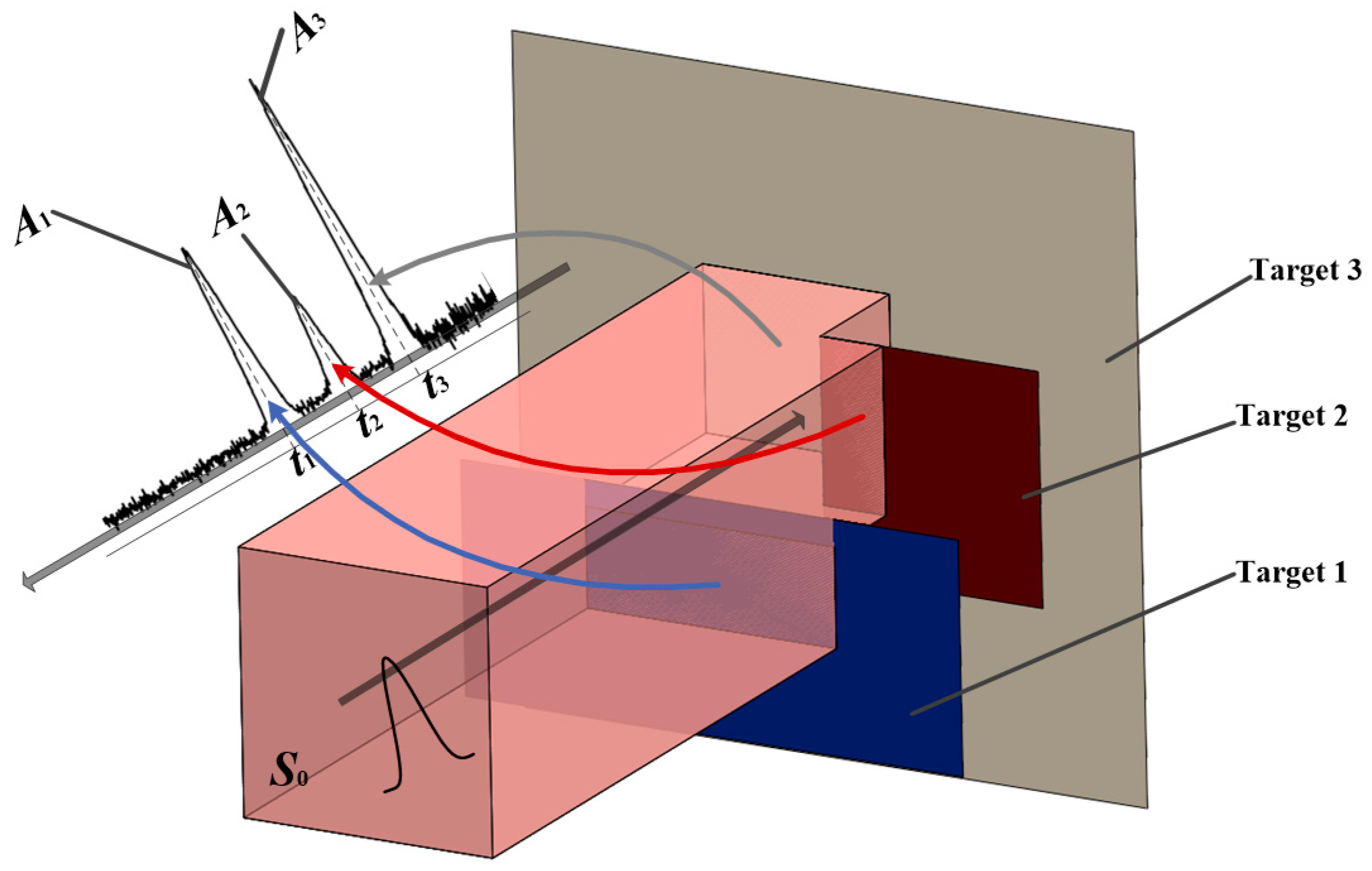
2. Multi Echoes in 3D Laser Imaging

The pulse emitted by the 3D laser imaging system is a Gaussian pulse, shown in Figure 1. The multi echoes received by the detector is expressed as [30].

$$P\left(t\right)={\displaystyle \sum _{i=1}^N{\eta }_s{\eta }_a}\frac{\pi d_r^2}{4R_i^2{S}_0}E\frac{\rho }{\mathsf{\Omega }}{A}_i\frac{{\sigma }_s}{\sqrt{{\sigma }_s^2+{\sigma }_i^2}}\exp \left(-\frac{{\left(t-t_i\right)}^2}{2\left({\sigma }_s^2+{\sigma }_i^2\right)}\right)$$

(1)

where, η_s is the system transmission factor and η_a is the atmospheric transmission factor, R_i is the range of the i-th scatterer, S₀ is the area of the projection spot, ρ is the reflectivity and A_i is the i-th receiving area of the scatter, d_r is the aperture diameter of the receiver optics, E is the original pulse energy, Ω is a cone of solid angle of scattered light, σ_s is the pulse width of the original pulse, σ_i is the received pulse width of the i-th pulse, t is the time, t_i = 2R_i/c is the time of flight (TOF) of the i-th echo.

The correlation terms with the area and distance of the target in Equation (1) are extracted, and other coefficients are taken as constants; then, the deformed formula is shown in Equation (2), where P_r is the total energy of the echo received by the detector and P_i is the energy of the i-th echo:

$$P_r={\displaystyle \sum _{i=1}^N{P}_i}$$

(2)

where,

$$P_i={\eta }_s{\eta }_a\frac{\pi d_r^2}{4R_i^2{S}_0}E\frac{\rho }{\mathsf{\Omega }}{A}_i\frac{1}{\sqrt{2}}\exp \left(-\frac{{\left(t-2R_i/c\right)}^2}{4{\sigma }_s^2}\right)$$

(3)

By further simplifying Equations (2) and (3), Equation (4) is inferred by Equations (2) and (3). Where M is the term that does not contain the distance and reflection area of the target, as shown in Equation (5). For the multi echoes generated by different targets under the same scanning spot, M is regarded as a constant.

$$P_i=M\frac{A_i}{R_i^2}\exp \left(-\frac{{\left(t-2R_i/c\right)}^2}{4{\sigma }_s^2}\right)$$

(4)

where,

$$M=\frac{\pi }{4\sqrt{2}}{\eta }_s{\eta }_a\frac{d_r^2}{S_0}E\frac{\rho }{\mathsf{\Omega }}$$

(5)

When assuming that the sensor can measure and recognize an arbitrary number of pulses and the reflectivity of the target is constant, the ratio of the reflection area of the i-th target and the sum of the reflection areas of each target is expressed as:

$${\tau }_i=\frac{A_i}{{\displaystyle \sum A_i}}=\frac{R_i^2\cdot P_i}{{\displaystyle \sum R_i^2\cdot P_i}}$$

(6)

Since R = c·t, Equation (6) is expressed as:

$${\tau }_i=\frac{c^2{t}_i^2\cdot P_i}{{\displaystyle \sum c^2{t}_i^2\cdot P_i}}=\frac{t_i^2\cdot P_i}{{\displaystyle \sum t_i^2\cdot P_i}}$$

(7)

By decomposing multi echoes, the TOF and echo intensity of each target are obtained. Then the PAET (τ_i) is obtained through Equation (7).

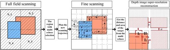
3. Scanning Strategy and Depth Image Reconstruction

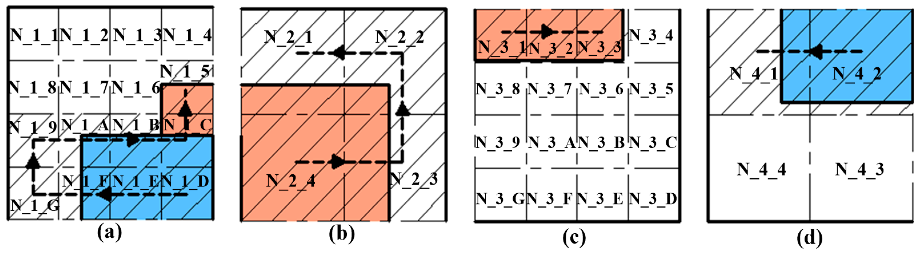
3.1. Scanning Strategy of Variable Scanning Spot and Scanning Trajectory

According to the fixed-size laser sport, the details of targets are difficult to obtain because of the unable difficulty of fully scanning the boundary of two objects. Therefore, setting the size of the scanning spot and planning a reasonable scanning trajectory can effectively reduce the number of scanning points. At the same time, the PAET is calculated according to the intensity and TOF of each echo in the multi echoes.

The scanning strategy to realize variable scanning spot and scanning trajectory is shown in Figure 2.

Step 1. Rough scanning. For the target with the area of S, set the scanning step of this region, i.e., T_i, where T is the flag of scanning order, and i is the i-th scanning step. Using the scanning spot with the area of D₁ = S/n² (n is the number of the sub-region of the target, n ≥ 2) to scan the target, shown in Figure 3a. Then the waveform processing and pulse extraction are carried out on the echo signal of each region received by the detector [31].

Step 2. RME classification. Calculate the reflection area (δ) of the smallest target in each RME. If δ > D₁/4ⁱ, such as N_2 and N_4 in Figure 3, the scanning step of these regions are marked as T_i + 1. If δ < D₁/4ⁱ, such as N_1 and N_3 in Figure 3, the scanning step of these regions are marked as T_i + 2.

Step 3. Scanning trajectory scheme. Plan the scanning trajectory of the region, whose scanning step is marked as T_i + 1. Such as N_2 in Figure 3b, the region N_2 is equally divided into four sub-regions. Subsequently, it is judged whether there are the same targets in the adjacent regions of N_2. As shown in Figure 3, two adjacent regions (N_1, N_3) of N_ 2 have the same echo of Target 2. Therefore, the scanning trajectory of the sub-region of N_2 starts from the N_2_4, which is close to N_1 and N_3, and the direction away from N_1 and N_3 is taken as the scanning direction. The scanning trajectory of the sub-region of N_2 is shown in Figure 4b. In the same way, the scanning trajectory of the sub-region of N_4 is planned with the same method.

Step 4. Fine scanning. According to the reduction of the size of the scanning spot, the area of the new scanning spot is D₂ = D₁/4ⁱ. Scanning the sub-regions of N_2 by using the scanning trajectory planned in step 3. When scanning each sub-region of N_2, the reflection area of each target in each sub-region is calculated and accumulated according to the echo signal. When the sum of the areas of the target in the scanned sub-region is greater than or equal to the total area of this target in N_2, the scanning of this region is completed, and the sub-regions of N_4 can be scanned in the same way. The scanning trajectory of sub-regions of N_2 and N_4 are shown in Figure 4b,d, respectively. Then, the scanning steps of the sub-areas with multi echoes in N_2 and N_4 are marked as T_i + 2.

Step 5. Repeat steps 2–4 until there is no RME, or the scanning spot is no longer reduced.

Step 6. Record the location and the PAET of all scanned regions.

Scanning points and scanning trajectories in each scanning step from T_1 to T_3 are shown in Figure 5.

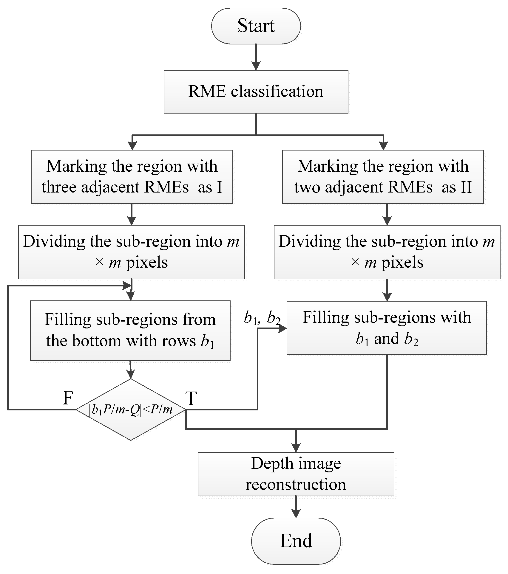
3.2. Super-Resolution Reconstruction of Depth Image

By scanning the target with the variable scanning spot and scanning trajectory, the number of targets in each sub-region and the PAET is obtained. Due to the influence of the scanning trajectory and the area of the scanning spot, the scanning spot usually covers the region with multi-targets. Therefore, the region of targets is divided into the region with single echo (RSE) and RME, as shown in Figure 6. For the region marked as ‘1′, there is one echo single in this region, and it can be uniquely reconstructed. If there are two targets in the region marked as ‘2’, this region cannot be uniquely reconstructed. However, the PAET and location of each target in the RME can be obtained by scanning with the above scanning strategy. Therefore, each target in the RME is restored more accurately by segmenting the region and filling the sub-region according to the PAET and the location of each target.

The method of depth image super-resolution reconstruction is shown in Figure 7.

Step 1. RME classification. The region with three adjacent RMEs is marked as “I”, such as the region I₁ and I₂ in Figure 6b. The region with two adjacent RMEs is marked as “II”.

Step 2. Region segmentation. For the RME with the area of P, set the number of sub-regions to be divided as m × m. After sub-region segmentation, the area of each sub-region is P/m².

Step 3. Edge region filling. The region marked as I is divided into m × m sub-regions, and these sub-regions are filled line by line from the bottom. As shown in Figure 6c, the number of rows b₁ is filled. If the difference between the filled area and the calculated area of this region (Q = τ_i ∙ P) satisfies |b₁P/m − Q| < P/m, record the number of pixels and rows in this filled sub-region.

Step 4. Corner region filling. The region marked as II is divided into m × m sub-regions. The row and column of the adjacent region are regarded as the boundary of the region to be filled. Such as region II showed in Figure 6b, the number of rows and columns (b₁, b₂) obtained from the two adjacent regions (I₁, I₂) is used as the boundary of the filled region to fill region II. The filling result is shown in Figure 6d.

Step 5. Depth image reconstruction. The depth image of RSE is enhanced to m × m pixels. Then the super-resolution depth image of the target is reconstructed by combining the depth images of RSE and the region I and II.

4. Experiment and Results

The experimental setup is shown in Figure 8. A summary of the system parameters is listed in

Table 1. Summary of the system parameters.

System Parameters	Values
Wavelength	532 nm
Laser Repetition Rate	10 kHz
Laser Pulse Width	1.5 ns
Average Output Power	500 mW
Receiving lens	f = 50 mm
Emission lens	f = 35 mm/f = 45 mm
Photosensitive surface of APD	3 × 3 mm2
Scanning speed	1 s/point

. The laser passes through the emission lens (EL), and the spot of the emission laser is expanded. The expanded laser is projected onto the surface of the target via a dual galvanometer (DG) which scans the target area directing the emission laser in the x and y planes. The laser pulse reflected by the target passes through the receiving lens (RL) and is received by APD.

The target is composed of two plates with the size of 0.45 × 0.24 m and 0.9 × 0.9 m respectively. The distance between the two plates is 3 m, shown in Figure 9.

The EL is adjusted to expand the emission laser, and the scanning spot with 180 × 180 mm is formed on the surface of the target. Using this scanning spot to scan the target, the reflected echoes of twenty-five sub-regions are obtained. The scanning time is 25 s. Using the method from Reference [31] to process the echo signal and calculating the PAET of target A in each RME, as shown in Figure 10a. Then the depth image is reconstructed according to the PAET in each sub-region. The depth image of the target with 5 × 5 pixels is shown in Figure 10b.

By changing the focal length of the EL, the size of the scanning spot is reduced to 90 × 90 mm. The new scanning spot is used to scan these RMEs in Figure 10a. The scanning trajectory of each sub-region is shown in Figure 11f. The scanning time is 18 s. The echo signal and PAET of each sub-region are shown in Figure 11a–e. In order to ensure that each sub-region of the target has the same number of pixels, the RSEs in Figure 10a are enhanced to 4 × 4 pixels. By combining the extended depth image of the RSEs with the depth image of RMEs, the depth image of the target with 10 × 10 pixels is obtained, as shown in Figure 12.

After scanning the RME in Figure 10a, there are still ten RMEs in the scanned sub-regions, as shown in Figure 11a–e. Therefore, we divide each RME into 16 × 16 sub-regions. Then using the proposed depth image reconstruction method to fill the area of each sub-region and reconstruct the depth image. Finally, we get a super-resolution depth image of the target with 160 × 160 pixels, as shown in Figure 13.

5. Discussion

We compare each reconstructed depth image with the real depth image of the target. The AOAR and SSIM [32] between each reconstructed depth image and the real depth image are shown in Figure 14.

From the comparison results, the AOAR and SSIM of each reconstructed depth image have obvious changes. There are several reasons for these changes.

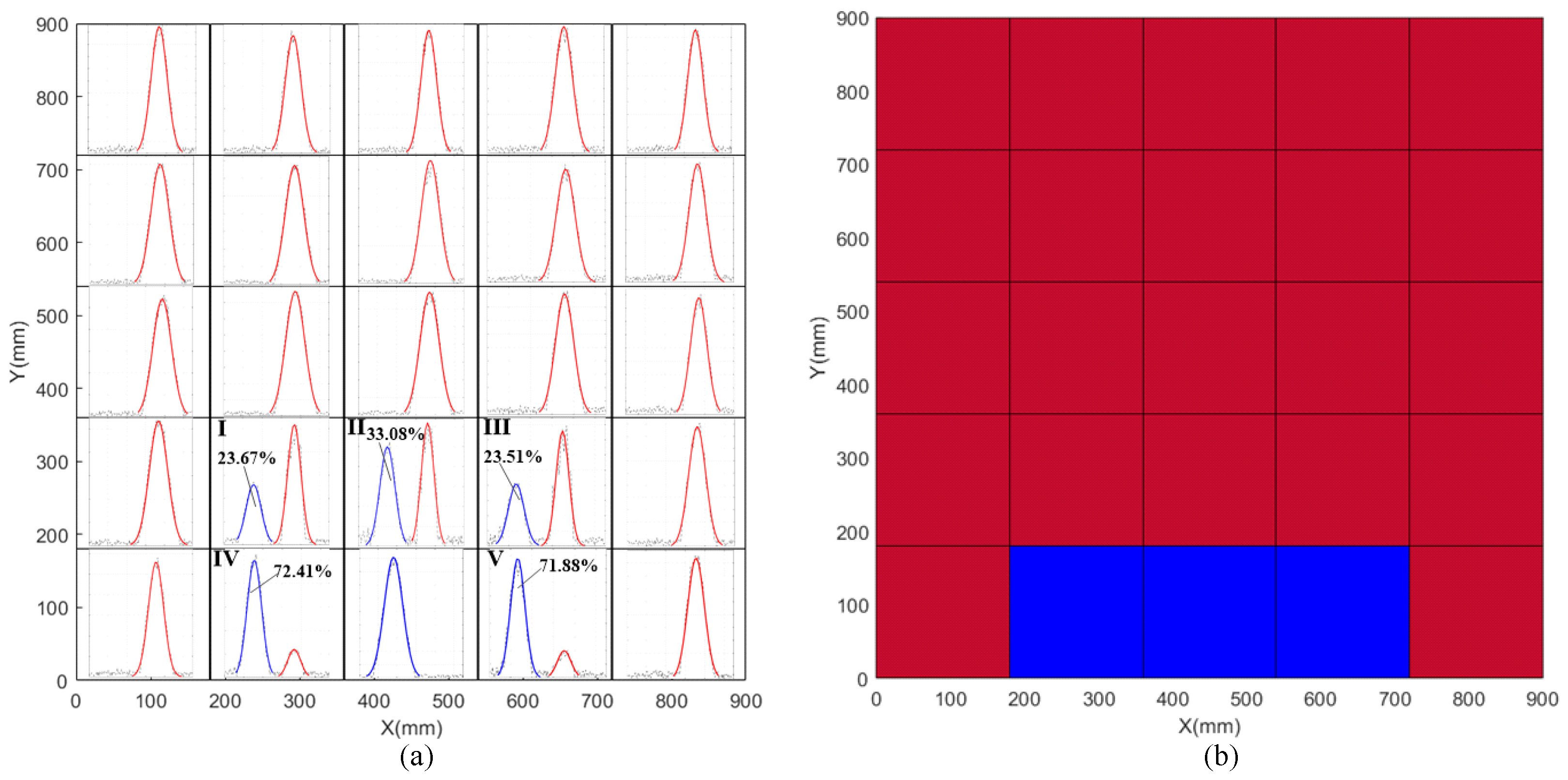
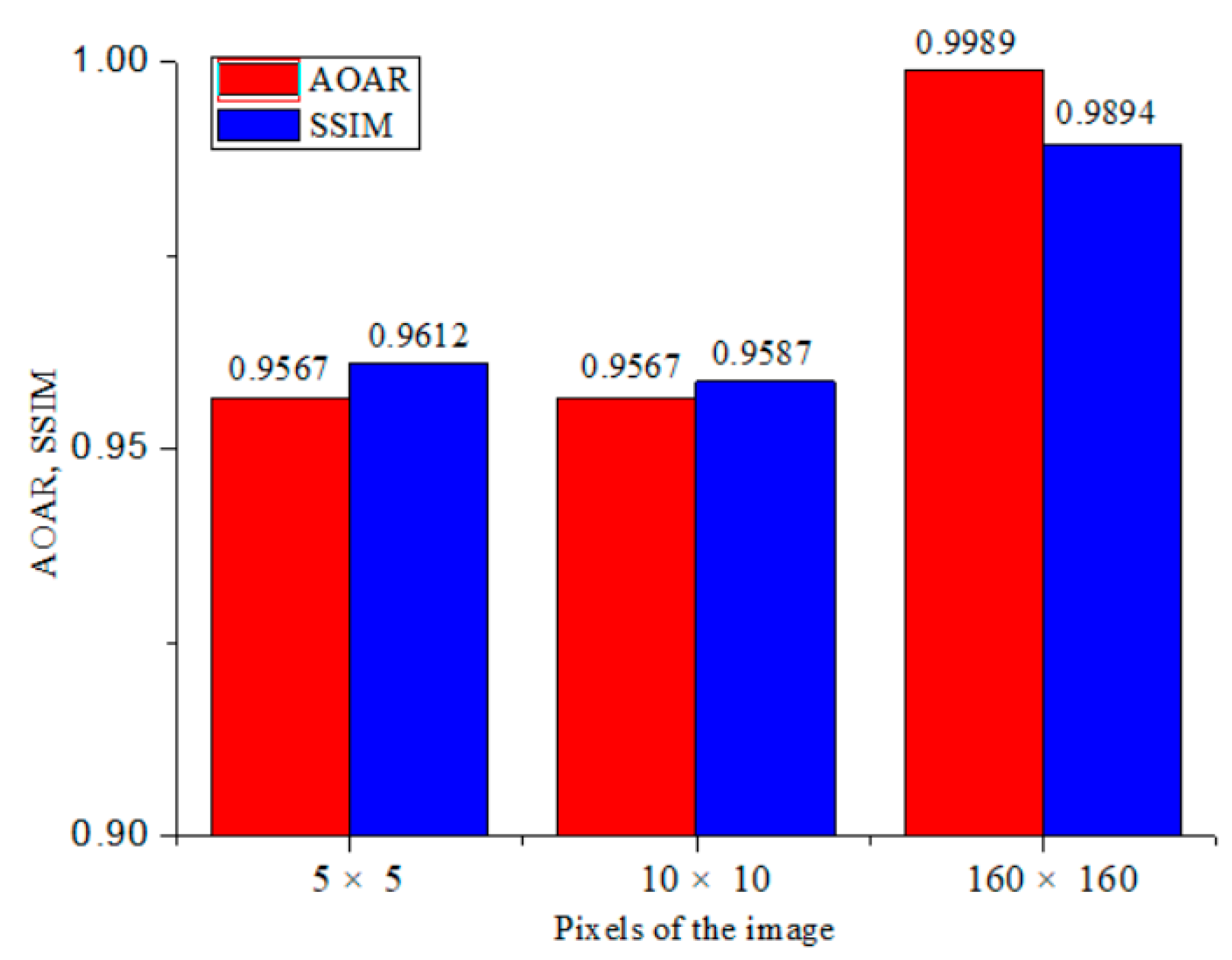
• When scanning the target with a large-scale scanning spot, a single scanning spot covers a large area of the target, which results in many RMEs. When an RME is represented by one pixel, this RME cannot be represented accurately. Therefore, the AOAR and SSIM of the reconstructed depth image with 5 × 5 pixels are relatively low.
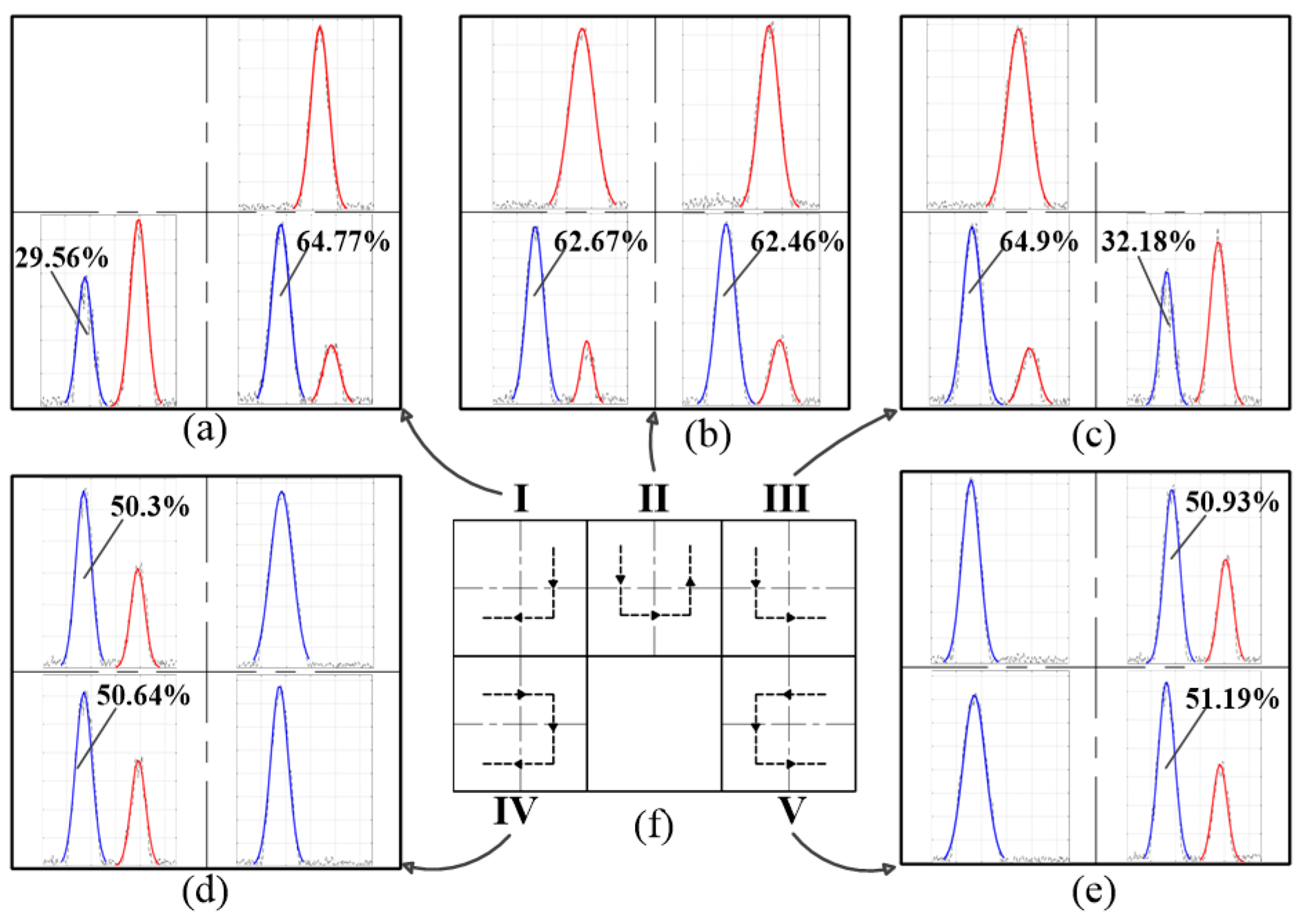
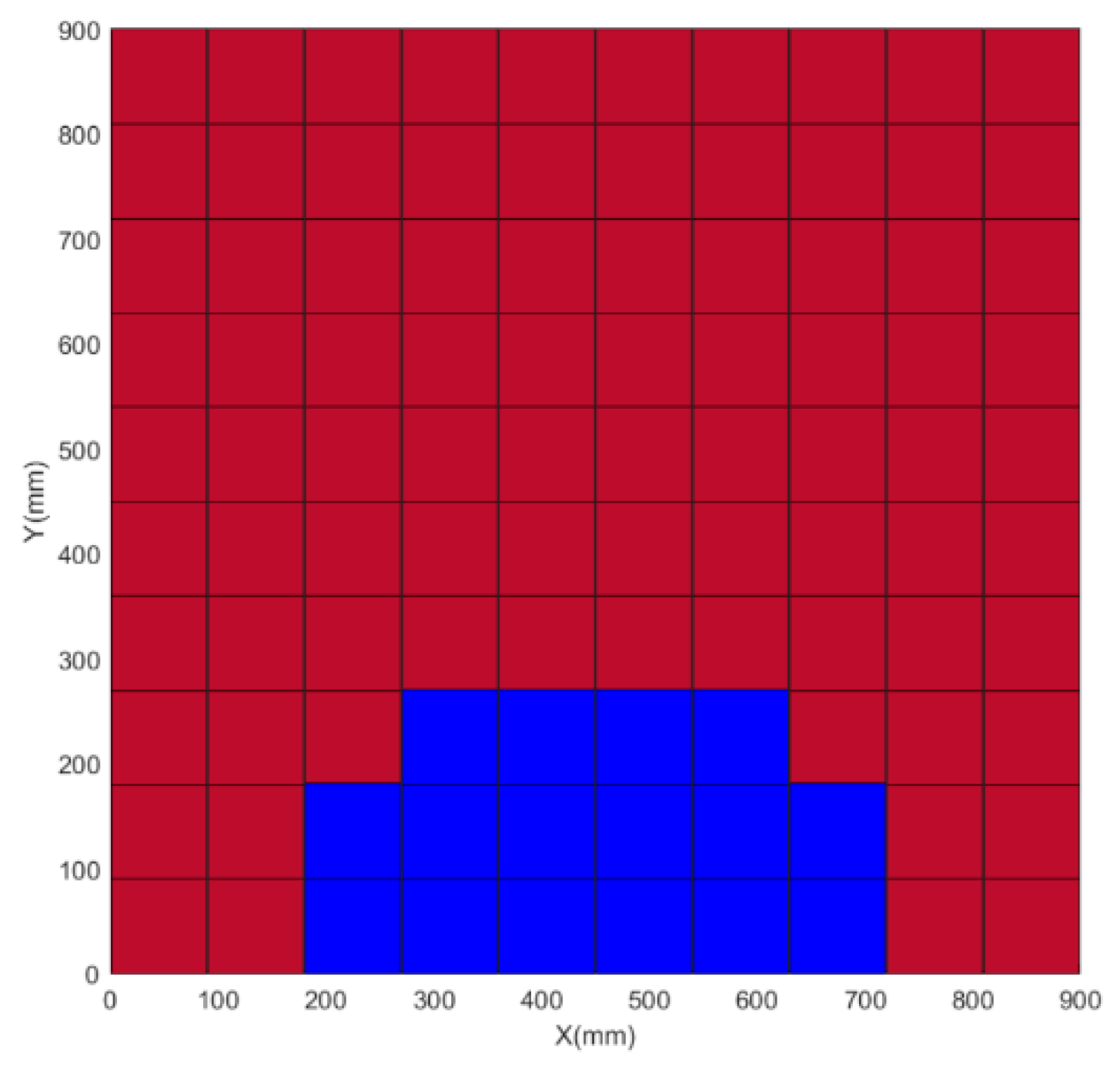
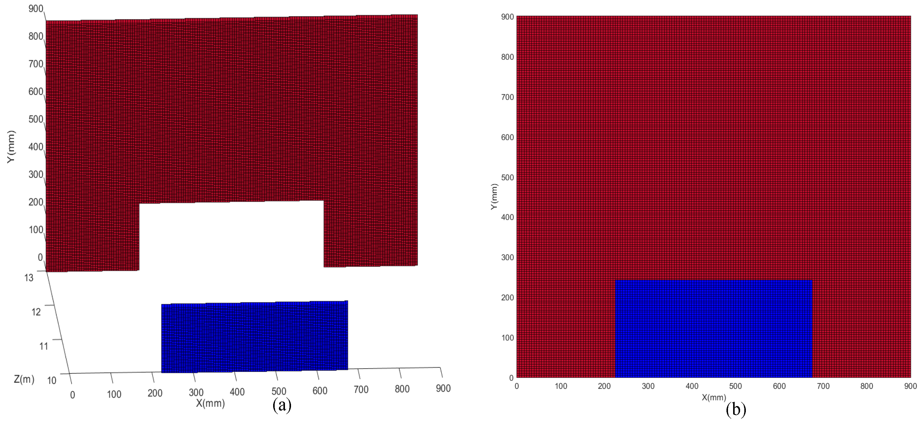
• When the size of the scanning spot is reduced and the RME is scanned more precisely with the new scanning spot, the number of the RME decreases. However, due to the influence of the small scanning spot and the newly scanning trajectory, the PAET at the edge has changed. Therefore, these RMEs at the edge cannot be accurately reconstructed. As shown in Figure 12, the edge of the blue region is missing. It leads to the decrease of the SSIM of the reconstructed depth image with 10 × 10 pixels.
• When the depth image is super-resolution reconstructed, the RME is reconstructed more accurately by segmenting the RME and filling the sub-region. Therefore, the reconstructed depth image with 160 × 160 pixels is consistent with the real depth image in terms of AOAR and SSIM.

In the experiment, the number of scanning points is 43, and the number of pixels of the reconstructed depth image is 160 × 160. Therefore, the sampling rate is only 0.17%, which is much better than the sampling rate in Reference [29].

However, it is obvious that the reflected echoes of the two targets overlap each other when the distance between two targets is less than R_m = c·τ₀/2 (c is the speed of light, τ₀ is the pulse width). Therefore, when the distance between two targets is less than R_m, lidar cannot distinguish two targets by the overlapping echo.

Meanwhile, in our previous research, we found that when the scanned target is curved and the target surface rotates, its echo peak, the center position of the echo, and the pulse width are changed [33]. We analyze the echo of the plane target and spherical target with a diameter of 180 mm. The echoes of the plane and sphere rotating at different angles are shown in Figure 15.

As shown in Figure 15a, when the plane is tilted, the pulse width of the echo is broadened, and the peak value of the echo decreases rapidly with the increase of the rotation angle. As shown in Figure 15b, when the curved surface target is tilted, the pulse width of the echo is also be broadened, and the center position of the echo is shifted. From the comparison of Figure 15a,b, the echo of the spherical target is broadened, and the peak value of the echo is reduced compared with that of the plane target.

In order to analyze the reason for the echo change in the width and peak shift, a laser beam is regarded as a set of five sub-rays (L1~L5). After each sub-ray is reflected by the target, these sub-rays are accumulated at the detector to form an echo of this laser beam. The echoes reflected from a plane and an inclined plane are shown in Figure 16a. When the plane is not tilted, the TOFs of the reflected echo of these sub-rays are the same. Therefore, the pulse width and the center position of the echo formed by the superposition of five sub-rays are not changed, as shown by the dotted line in Figure 16a. When the plane rotates an angle counterclockwise, the optical paths of L1 and L2 increase, i.e., the TOF increase, while the optical paths of L4 and L5 decrease, i.e., the TOF decrease. The central position of the echo of each sub-ray, therefore, is separated, and the pulse width of the echo accumulated of five sub-rays is broadened, as shown by the black solid line in Figure 16a. The echoes reflected from a sphere and an inclined sphere are shown in Figure 16b. Similarly, when the sphere rotates an angle counterclockwise, the optical path of each sub-ray is changed, which leads to the pulse width broadening of the echo accumulated of five sub-rays. In contrast to the case where the plane is tilted, the height of each point on the spherical surface is not the same. When the sphere is tilted, the absolute values of the changed optical paths of L1 and L2 are not equal to that of L4 and L5. It causes the center position of the echo accumulated of five sub-rays to be shifted, as shown by the black solid line in Figure 16b.

Therefore, when a curved or inclined target is scanned and imaged, the echoes of these targets occur in deformation. The depth and reflection area of the target extracted from the echo are less than their true values. It reduces the accuracy of the reconstructed depth image by using the proposed depth image super-resolution reconstruction method. Therefore, it is necessary to further study the characteristics of multi echoes in complex scenes and improve the accuracy of the range and reflection area of the target extracted from the multi echoes to adapt to target scanning and depth image super-resolution reconstruction in complex scenes.

6. Conclusions

In this paper, we propose a scanning and depth image reconstruction method with variable the scanning spot and scanning trajectory. This method obtains the location and area of each target in the scanned region based on the TOF and the echo intensity contained in the multi echoes of this region. Firstly, the location and area of RME are obtained by scanning the target with a large scanning spot. Then, by reducing the size of the scanning spot and planning a new scanning trajectory, the RME is scanned precisely, and the PAET in each RME is obtained. Through the scanning and imaging experiment of the target composed of two plates, we reconstruct the super-resolution depth image of the target with 160 × 160 pixels by scanning the target with only forty-three points. Compared with the real depth image of the target, the AOAR and SSIM of the reconstructed depth image are 99.89% and 98.94%, respectively. Therefore, the scanning and image reconstruction method proposed in this paper can significantly reduce the number of scanning points, improve the scanning efficiency, and improve the AOAR and SSIM of the reconstructed depth image. In addition, the low accuracy of the range and reflection area of the target extracted from multi echoes will reduce the accuracy of the reconstructed depth image by using the proposed depth image super-resolution reconstruction method. Therefore, in the following work, we will study the signal processing and extraction method of complex echo in complex scenes to apply the proposed method in complex scenes.

References

1. Lee, J.; Kim, Y.-J.; Lee, K.; Lee, S.; Kim, S.-W. Time-of-flight measurement with femtosecond light pulses. Nat. Photonics 2010, 4, 716–720. [Google Scholar] [CrossRef]
2. Wang, B.; Song, S.; Gong, W.; Cao, X.; He, D.; Chen, Z.; Lin, X.; Li, F.; Sun, J. Color Restoration for Full-Waveform Multispectral LiDAR Data. Remote Sens. 2020, 12, 593. [Google Scholar] [CrossRef] [Green Version]
3. Chan, T.K.; Megens, M.; Yoo, B.W.; Wyras, J.; Chang-Hasnain, C.J.; Wu, M.C.; Horsley, D.A. Optical beamsteering using an 8 × 8 MEMS phased array with closed-loop interferometric phase control. Opt. Express 2013, 21, 9. [Google Scholar] [CrossRef] [PubMed]
4. Li, Z.-P.; Huang, X.; Jiang, P.-Y.; Hong, Y.; Yu, C.; Cao, Y.; Zhang, J.; Xu, F.; Pan, J.-W. Super-resolution single-photon imaging at 82 km. Opt. Express 2020, 28. [Google Scholar] [CrossRef] [Green Version]
5. McCarthy, A.; Collins, R.J.; Krichel, N.J.; Fernández, V.; Wallace, A.M.; Buller, G.S. Long-range time-of-flight scanning sensor based on high-speed time-correlated single-photon counting. Appl. Opt. 2009, 48, 6241–6251. [Google Scholar] [CrossRef] [Green Version]
6. Wallace, A.M.; Ye, J.; Krichel, N.J.; McCarthy, A.; Collins, R.J.; Buller, G.S. Full Waveform Analysis for Long-Range 3D Imaging Laser Radar. Eurasip J. Adv. Signal Process. 2010, 2010. [Google Scholar] [CrossRef] [PubMed] [Green Version]
7. Andresen, B.F.; Jack, M.; Chapman, G.; Edwards, J.; Mc Keag, W.; Veeder, T.; Wehner, J.; Roberts, T.; Robinson, T.; Neisz, J.; et al. Advances in ladar components and subsystems at Raytheon. In Infrared Technology and Applications XXXVIII; International Society for Optics and Photonics: San Diego, CA, USA, 2012; Volume 8353, p. 83532F. [Google Scholar]
8. Itzler, M.A.; Verghese, S.; Campbell, J.C.; McIntosh, K.A.; Liau, Z.L.; Sataline, C.; Shelton, J.D.; Donnelly, J.P.; Funk, J.E.; Younger, R.D.; et al. Arrays of 128 × 32 InP-based Geiger-mode avalanche photodiodes. In Advanced Photon Counting Techniques III; International Society for Optics and Photonics: San Diego, CA, USA, 2009; Volume 7320, p. 73200M. [Google Scholar]
9. Pawlikowska, A.M.; Halimi, A.; Lamb, R.A.; Buller, G.S. Single-photon three-dimensional imaging at up to 10 km range. Opt. Express 2017, 25. [Google Scholar] [CrossRef]
10. Yang, X.; Su, J.; Hao, L.; Wang, Y. Optical OCDMA coding and 3D imaging technique for non-scanning full-waveform LiDAR system. Appl. Opt. 2019, 59. [Google Scholar] [CrossRef]
11. Li, Y.; Ibanez-Guzman, J. Lidar for Autonomous Driving: The Principles, Challenges, and Trends for Automotive Lidar and Perception Systems. IEEE Signal Process. Mag. 2020, 37, 50–61. [Google Scholar] [CrossRef]
12. Liu, X.; Sun, X.; Xia, X. LiDAR point’s elliptical error model and laser positioning for autonomous vehicles. Meas. Sci. Technol. 2021, 32. [Google Scholar] [CrossRef]
13. Schwarz, B. Mapping the world in 3D. Nat. Photonics 2010, 4, 429–430. [Google Scholar] [CrossRef]
14. Morales, J.; Plaza-Leiva, V.; Mandow, A.; Gomez-Ruiz, J.A.; Serón, J.; García-Cerezo, A. Analysis of 3D Scan Measurement Distribution with Application to a Multi-Beam Lidar on a Rotating Platform. Sensors 2018, 18, 395. [Google Scholar] [CrossRef] [PubMed] [Green Version]
15. Ravi, R.; Lin, Y.-J.; Elbahnasawy, M.; Shamseldin, T.; Habib, A. Bias Impact Analysis and Calibration of Terrestrial Mobile LiDAR System With Several Spinning Multibeam Laser Scanners. IEEE Trans. Geosci. Remote Sens. 2018, 56, 5261–5275. [Google Scholar] [CrossRef]
16. Hu, T.; Sun, X.; Su, Y.; Guan, H.; Sun, Q.; Kelly, M.; Guo, Q. Development and Performance Evaluation of a Very Low-Cost UAV-Lidar System for Forestry Applications. Remote Sens. 2020, 13, 77. [Google Scholar] [CrossRef]
17. Amani, M.; Mahdavi, S.; Berard, O. Supervised wetland classification using high spatial resolution optical, SAR, and LiDAR imagery. J. Appl. Remote Sens. 2020, 14. [Google Scholar] [CrossRef]
18. Zhang, Y.; Sun, Z.; Chen, S.; Chen, H.; Guo, P.; Chen, S.; He, J.; Wang, J.; Nian, X. Classification and source analysis of low-altitude aerosols in Beijing using fluorescence–Mie polarization lidar. Opt. Commun. 2021, 479. [Google Scholar] [CrossRef]
19. Akbulut, M.; Kotov, L.; Wiersma, K.; Zong, J.; Li, M.; Miller, A.; Chavez-Pirson, A.; Peyghambarian, N. An Eye-Safe, SBS-Free Coherent Fiber Laser LIDAR Transmitter with Millijoule Energy and High Average Power. Photonics 2021, 8, 15. [Google Scholar] [CrossRef]
20. Kirmani, A.; Venkatraman, D.; Shin, D.; Colaço, A.; Wong, F.N.; Shapiro, J.H.; Goyal, V.K. First-photon imaging. Science 2014, 343, 58–61. [Google Scholar] [CrossRef]
21. McCarthy, A.; Ren, X.; Della Frera, A.; Gemmell, N.R.; Krichel, N.J.; Scarcella, C.; Ruggeri, A.; Tosi, A.; Buller, G.S. Kilometer-range depth imaging at 1550 nm wavelength using an InGaAs_InP single-photon avalanche. Opt. Express 2013, 21, 16. [Google Scholar] [CrossRef] [Green Version]
22. Zheng, T.; Shen, G.; Li, Z.; Yang, L.; Zhang, H.; Wu, E.; Wu, G. Frequency-multiplexing photon-counting multi-beam LiDAR. Photonics Res. 2019, 7. [Google Scholar] [CrossRef]
23. Poulton, C.V.; Yaacobi, A.; Cole, D.B.; Byrd, M.J.; Raval, M.; Vermeulen, D.; Watts, M.R. Coherent solid-state LIDAR with silicon photonic optical phased arrays. Opt. Lett. 2017, 42. [Google Scholar] [CrossRef] [PubMed]
24. Lio, G.E.; Ferraro, A. LIDAR and Beam Steering Tailored by Neuromorphic Metasurfaces Dipped in a Tunable Surrounding Medium. Photonics 2021, 8, 65. [Google Scholar] [CrossRef]
25. Li, Z.; Wu, E.; Pang, C.; Du, B.; Tao, Y.; Peng, H.; Zeng, H.; Wu, G. Multi-beam single-photon-counting three-dimensional imaging lidar. Opt. Express 2017, 25. [Google Scholar] [CrossRef] [PubMed]
26. Kamerman, G.W.; Marino, R.M.; Davis, W.R.; Rich, G.C.; McLaughlin, J.L.; Lee, E.I.; Stanley, B.M.; Burnside, J.W.; Rowe, G.S.; Hatch, R.E.; et al. High-resolution 3D imaging laser radar flight test experiments. In Laser Radar Technology and Applications X; International Society for Optics and Photonics: San Diego, CA, USA, 2005; Volume 5791, pp. 138–151. [Google Scholar]
27. Li, S.; Cao, J.; Cheng, Y.; Meng, L.; Xia, W.; Hao, Q.; Fang, Y. Spatially Adaptive Retina-Like Sampling Method for Imaging LiDAR. IEEE Photonics J. 2019, 11, 1–16. [Google Scholar] [CrossRef]
28. Cheng, Y.; Cao, J.; Zhang, F.; Hao, Q. Design and modeling of pulsed-laser three-dimensional imaging system inspired by compound and human hybrid eye. Sci. Rep. 2018, 8. [Google Scholar] [CrossRef]
29. Ye, L.; Gu, G.; He, W.; Dai, H.; Lin, J.; Chen, Q. Adaptive Target Profile Acquiring Method for Photon Counting 3-D Imaging Lidar. IEEE Photonics J. 2016, 8, 1–10. [Google Scholar] [CrossRef]
30. Wagner, W.; Ullrich, A.; Ducic, V.; Melzer, T.; Studnicka, N. Gaussian decomposition and calibration of a novel small-footprint full-waveform digitising airborne laser scanner. Isprs J. Photogramm. Remote Sens. 2006, 60, 100–112. [Google Scholar] [CrossRef]
31. Hofton, M.A.; Minster, J.B.; Blair, J.B. Decomposition of laser altimeter waveforms. IEEE Trans. Geosci. Remote Sens. 2000, 38, 1989–1996. [Google Scholar] [CrossRef]
32. Wang, Z.; Bovik, A.C.; Sheikh, H.R.; Simoncelli, E.P. Image Quality Assessment: From Error Visibility to Structural Similarity. IEEE Trans. Image Process. 2004, 13, 600–612. [Google Scholar] [CrossRef] [Green Version]
33. Hao, Q.; Cheng, Y.; Cao, J.; Zhang, F.; Zhang, X.; Yu, H. Analytical and numerical approaches to study echo laser pulse profile affected by target and atmospheric turbulence. Opt. Express 2016, 24, 25026–25042. [Google Scholar] [CrossRef] [Green Version]
Figure 1. TOF measurement of multi-target.
Photonics 08 00173 g001
Figure 2. The scanning strategy with the variable scanning spot and scanning trajectory.
Photonics 08 00173 g002
Figure 3. (a) Sub-region segmentation and the echo of each sub-region in the scanning step of T_1. (be) The multi echoes of the region N_1–N_4.
Photonics 08 00173 g003
Figure 4. (ad) The divided sub-regions and scanning trajectories of the region N_1–N_4.
Photonics 08 00173 g004
Figure 5. (ac) Scanned sub-regions and scanning trajectories in the scanning step from T_1 to T_3.
Photonics 08 00173 g005
Figure 6. Region segmentation and pixel filling. (a) Sub-regions with single echo and multi echoes. (b) Partial enlargement of (a). (ce) Sub-region segmentation and pixel filling of the region I1, II, and I2.
Photonics 08 00173 g006
Figure 7. The method of depth image super-resolution reconstruction.
Photonics 08 00173 g007
Figure 8. The experimental setup of 3D laser imaging system.
Photonics 08 00173 g008
Figure 9. Imaged targets. (a) Relative location of two plates. (b) Front view of (a).
Photonics 08 00173 g009
Figure 10. (a) The echo signal and PAET of each sub-region. (b) The depth image of the target with 5 × 5 pixels.
Photonics 08 00173 g010
Figure 11. (ae) Echo signals and PAETs of each sub-region. (f) The scanning trajectories of each sub-region in (ae).
Photonics 08 00173 g011
Figure 12. The depth image of the target with 10 × 10 pixels.
Photonics 08 00173 g012
Figure 13. (a) The depth image of the target with 160 × 160 pixels. (b) Front view of (a).
Photonics 08 00173 g013
Figure 14. The AOAR and SSIM between the reconstructed depth image and real depth image.
Photonics 08 00173 g014
Figure 15. The echoes of different targets rotating at different angles. (a) A plane; (b) A sphere.
Photonics 08 00173 g015
Figure 16. The echoes and the superimposed echo of five sub-rays of different targets. (a) A plane and an inclined plane; (b) A sphere and an inclined sphere.
Photonics 08 00173 g016