Phase-Shifting Projected Fringe Profilometry Using Binary-Encoded Patterns

Abstract

A phase unwrapping method for phase-shifting projected fringe profilometry is presented. It did not require additional projections to identify the fringe orders. The pattern used for the phase extraction could be used for phase unwrapping directly. By spatially encoding the fringe patterns that were used to perform the phase-shifting technique with binary contrasts, fringe orders could be discerned. For spatially isolated objects or surfaces with large depth discontinuities, unwrapping could be identified without ambiguity. Even though the surface color or reflectivity varied periodically with position, it distinguished the fringe order very well.

1. Introduction

Phase-shifting projected fringe profilometry is a powerful tool in many profiling applications [1,2,3,4,5]. It sequentially projects a set of single-frequency patterns in which one differs from the others with a known shifted phase onto the inspected object. The sequent projections on the inspected surface are recorded using an image sensor array from another view angle. The phase of the projected fringes is distorted by the surface profile and, hence, the retrieved surface profile is analyzable. In the task of phase extraction, an arctangent operation is employed, making the phase being wrapped modulo 2π. Consequently, unwrapping is required to recover the absolute phase distribution.

Many unwrapping algorithms were presented for phase-shifting projected fringe profilometry [6,7,8,9,10,11,12,13,14,15,16,17,18,19]. In the methods that are used for multi-frequency projections [6,7,8,9,10,11], two or more sinusoidal fringe patterns with different frequencies are successfully projected onto the inspected surface. The phases of the projected patterns are extracted by the phase-shifting technique. Unwrapping is then performed by comparing all the wrapped phases. In the methods that employ temporally structured illuminations to identify fringe orders [12,13,14,15,16,17,18,19], the inspected object is sequentially illuminated by an additional set of gray-coding [12,13,14,15,16] or phase-coding [17,18,19] patterns. The temporal illuminations form a unique codeword for each fringe order. Unwrapping is then performed with reference to the fringe orders. However, these methods require additional temporal projections for phase unwrapping, hence requiring a longer measurement time. To reduce the number of additional projections, an alternative solution is the employment of a spatially encoded projection [20,21,22,23]. It spatially encodes fringes with different colors or quantized gray levels. Fringe orders are discerned via the permutation of the encoded fringes. However, ambiguities always occur when the surface is textured with various colors.

Our previous work proposed a binary-encoded method for phase unwrapping [23]. The binary-encoded method was developed based on the spatially encoded projection but it is more reliable at discerning fringes for surfaces with color or reflectance discontinuities. A fringe is recorded as “1” if its local minimum gray level is equal to half of the local maximum. By contrast, a fringe is recorded as “0” if its local maximum gray level is much larger than the local minimum. Then, this fringe pattern is recorded using a stream of binary digits. The permutation of binary digits is unique. Hence, fringe orders can be discerned with reference to the binary permutation. However, uncertainties might occur when the surface color or reflectivity is periodically distributed [23].

In this study, each fringe pattern that was used to perform the phase-shifting technique was encoded with the binary-encoding method. The number of additional projections (to identify fringe orders) was reduced to zero. Our original purpose was to maintain the advantages of the binary-encoding method (i.e., more reliable for surfaces textured with color or reflectivity discontinuities) and to minimize the number of projections (i.e., no need to take additional projections for phase unwrapping). The experimental results showed that it provided better performances than our expectation. The fringe contrast could also be extracted using the phase-shifting algorithm. It supplied additional information that allowed for analyzing the surface reflectivity. Hence, it is more flexible in applications that have surfaces with complicated color/reflectance distributions.

2. Materials and Methods

2.1. Fringe Encodingfor Phase-Shifting Projected Fringe Profilometry

Figure 1 shows the optical configuration of the profile measurements. A set of binary-encoded fringe patterns that were used to perform the phase-shifting technique were employed as the input signals to the digital projector. With a projector lens, these patterns (located on the x_p–y_p plane) were sequentially mapped to the inspected object positioned in the (x, y, z) coordinates. The fringes on the object were recorded using a CCD camera, in which the recorded images were focused on the x_d–y_d plane.

The binary-encoded fringe patterns can be mathematically expressed as

$$I_p{}^{(k)}(x_p,y_p)={\displaystyle \sum _{n=1}^N{I}_m{}^{(k)}(x_p-n{T}_p,y_p)},$$

(1)

where m is the subscript representing a binary digit (i.e., 0 or 1), I_m is the gray level of the binary-encoded fringe, T_p is the fringe period in the x_p–y_p plane, n is the fringe order, N is the total number of fringes, and (k) is the superscript indicating that this encoded fringe is used to assemble the kth fringe pattern. For a five-step phase-shifting algorithm (i.e., k = 1, 2, …,5), each binary-encoded fringe I_m is expressed as

$$I_m{}^{(k)}(x_p,y_p)=\left\{\begin{array}{l}{A}_m[1+C_m\cos (2\pi x_p/T_p-2\pi (k-1)/5)],\mathrm{if}0\le x_p<T_p\\ {0,}_{}\hspace{1em}\hspace{1em}\hspace{1em}\hspace{1em}\hspace{1em}\hspace{1em}\hspace{1em}\hspace{1em}\hspace{1em}\hspace{1em}\hspace{1em}\hspace{1em}\hspace{1em}\mathrm{if}{x}_p<0,\mathrm{or}{x}_p\ge T_p\end{array}\right.,$$

(2)

where A_m is the DC bias and C_m is the fringe’s contrast ratio, which is defined as the amplitude divided by the DC gray level. In Equation (2), the phase of the fringe is expressed as φ_p = 2πx_p/T_p. A_m and C_m were further quantized into two levels, as given by

$$A_m=\left\{\begin{array}{l}125,\mathrm{if}m=0\\ 169,\mathrm{if}m=1\end{array}\right.,\mathrm{and}{C}_m=\left\{\begin{array}{l}0.80,\mathrm{if}m=0\\ 0.33,\mathrm{if}m=1\end{array}\right..$$

(3)

Based on Equation (3), all the fringe’s maximum gray levels were 225, but the local minimum gray levels were quantized into two levels, 25 and 113. Consequently, the fringe that is projected on the inspected object can be recognized as a “0” or “1” digit by evaluating either the local minimum gray level or the contrast ratio. Figure 2a shows a list of the fringe orders n with assigned binary digits m. Such an arrangement caused the five fringe patterns to be labeled with a long stream of binary digits, as shown in Figure 2b. In this stream, any six adjacent digits formed a codeword. Each codeword took place once in the entire stream. Based on the permutation rule, a total of 64 codewords (i.e., 2⁶ = 64) were created. Hence, a stream of 69 digits was produced (i.e., N = 69). Figure 3 shows the 1D gray-level distributions of the five binary-encoded patterns. Their 1D contrast distribution and phase distribution wrapped in the interval (0, 2π] are illustrated in Figure 4a,b, respectively. At the boundaries between the “0”- and “1”-encoded fringes, the changes in the DC gray levels and contrast ratios caused the gray-level distributions to be discontinuous, as the circled areas shown in Figure 3. By contrast, the gray-level distribution of the first encoded pattern (i.e., k = 1) was continuous because all the fringes’ maximum gray levels (with the same value of 225) were coincidentally located at the boundaries.

2.2. Relationships between the Input and Observed Gray Levels

In our system, the digital projector Epson EB-U04 (with a resolution of 1920 × 1200) and the 12-bit CCD camera PCO pixelfly qe (with a resolution of 1392 × 1024) were employed to perform the tasks of pattern projection and image acquisition, respectively. To evaluate the linearity between the input gray level I_p (to the digital projector) and the gray-level I_d (recorded by the digital camera), a screen that was textured with various reflection coefficients, as shown in Figure 5a, was selected as the inspected object. The digital projector successively illuminated the screen with various input gray levels I_p. Each illumination on the screen was sequentially recorded by the CCD camera with a given exposure time and a given lens aperture. Figure 5b shows the obtained data sets and fitted curves for the sampled pixels illustrated in Figure 5a. The correspondences between the input and the observed gray levels contained nonlinear errors. A couple of methods were presented to cope with the linear distortion [24,25,26]. Here, we simply confined the input gray level I_p within the range from 25 to 225 to sustain the linearity. Figure 5c shows the fitted relationships in the linear area. They can be simply described as

$$I_d=a+b·I_p,25\le I_p\le 225,$$

(4)

where the parameters a and b are constant values. More specifically, parameter b changed with the surface reflectance but parameter a was approximately −32 for most sampled points, except for the sampled pixel marked with the cyan frame. The reason can be seen in Figure 5d, which illustrates the relationships between the normalized I_d and the input gray level I_p. Most of the fitted lines were overlapped, except for the cyan one. The observed signal at the pixel marked with the cyan frame was so weak that the background noise was not negligible, resulting in a correspondence that was smeared by background noises. Note that these noises were negligible for surfaces whose reflection coefficients were higher than that sampled at the magenta-framed pixel. To evaluate the change in linear relationships caused by the background noises, a close-up view for the sampled pixels marked with the magenta frame and the cyan frame is shown in Figure 5e. Three other linear correspondences that were smeared by background noises are added and plotted with dashed lines. They were measured from another three surfaces whose reflection coefficients were higher than that measured at the cyan-framed pixel. As a reference, the relationships between the normalized I_d and the input gray level I_p are shown in Figure 5f.

Based on Figure 5c,e, the linear relationships could be divided into two cases: the case of high reflectance surfaces and the case of low reflectance surfaces. For surfaces with high reflection coefficients, background noises were negligible and their parameter a described in Equation (3) was approximately −32. Moreover, as shown in Figure 5c, the maximum gray level I_d sampled at the magenta-framed pixel was approximately 1130. Consequently, for high-reflectance surfaces, an input gray level of I_p = 225 always caused the observed gray level I_d to be larger than 1130. By contrast, for surfaces with low reflection coefficients, an input gray level I_p = 225 caused the observed gray level I_d to be smaller than 1130, and an input gray level I_p = 25 caused the observed gray level I_d to range from 90 to 120, as shown in Figure 5e.

2.3. The Method Used forFringe Decodingand Unwrapping

The binary-encoded patterns whose 1D gray-level distributions are shown in Figure 3 were projected onto the inspected object. The minimum and maximum gray levels shown in Figure 3 are 25 and 225, respectively. Consequently, the projected pattern that was observed by the digital camera, I_d^(k), was a fairly linear response to the encoded patterns I_p^(k). The gray levels of the five recorded images can be described as

$$I_d{}^{(k)}(x_d,y_d)=A_d(x_d,y_d)+B_d(x_d,y_d)\cos \left[\varphi (x_d,y_d)-2\pi (k-1)/5\right],$$

(5)

where (k) is the superscript used to address the kth image (i.e., k = 1, 2, …, 5), A_d is the DC gray level, B_d is the fringe amplitude, and φ is the phase of the projected fringes. The parameters A_d, B_d, and φ can respectively be obtained using

$$A_d(x_d,y_d)=\frac{1}{5}{\displaystyle \sum _{k=1}^5{I}_d{}^{(k)}(x_d,y_d)},$$

(6)

$$B_d(x_d,y_d)=\frac{2}{5}\sqrt{{\left[{\displaystyle \sum _{k=1}^5{I}_d{}^{(k)}(x_d,y_d)}\sin \left(2(k-1)\pi /5\right)\right]}^2+{\left[{\displaystyle \sum _{k=1}^5{I}_d{}^{(k)}(x_d,y_d)}\cos \left(2(k-1)\pi /5\right)\right]}^2},$$

(7)

$${\varphi }_{\mathrm{w}}(x_d,y_d)={\tan }^{-1}\left[\frac{{\displaystyle \sum _{k=1}^5{I}_d{}^{(k)}(x_d,y_d)}\sin \left(2(k-1)\pi /5\right)}{{\displaystyle \sum _{k=1}^5{I}_d{}^{(k)}(x_d,y_d)}\cos \left(2(k-1)\pi /5\right)}\right].$$

(8)

The subscript “w” in Equation (8) represents the phase wrapped in the interval (0, 2π].

By substituting Equation (2) into Equation (4), the gray levels of the observed fringe I_m′^(k) can be represented as

$$I_{m\text{'}}{}^{(k)}(x_d,y_d)=\left\{\begin{array}{l}(a+A_{m}b)[1+\frac{A_m{C}_{m}b}{a+A_{m}b}\cos (\frac{2\pi x_p}{T_p}-2\pi (k-1)/5)],\mathrm{if}0\le x_p<T_p\\ 0,\hspace{1em}\hspace{1em}\hspace{1em}\hspace{1em}\hspace{1em}\hspace{1em}\hspace{1em}\hspace{1em}\hspace{1em}\hspace{1em}\hspace{1em}\hspace{1em}\hspace{1em}\mathrm{if}{x}_p<0,\mathrm{or}{x}_p\ge T_p\end{array}\right.,$$

(9)

where the subscript m′ is the binary digit that needs to be decoded. By substituting Equation (3) into Equation (9), the observed contrast, which is defined as the fraction of the extracted amplitude and the DC gray level, can be expressed as

$$C_d(x_d,y_d)=\left\{\begin{array}{l}\frac{0.80·125b}{a+125b},\mathrm{if}m=0\\ \frac{0.33·169b}{a+169b},\mathrm{if}m=1\end{array}\right..$$

(10)

For high-reflectance surfaces, the parameter a is always much smaller than 125b or 169b. This led to C_d(x_d, y_d) being approximately equal to C_m. In such a situation, there are two ways to decode the projected fringe. The first one is to analyze the first pattern projection (i.e., k =1) with the decoding method described in a previous work [23]: A fringe is decoded as “1” if the gray level at φ_w = π is close to half of the gray level at φ_w = 0 or 2π. By contrast, a fringe is “0” if the gray level at φ_w = π is much smaller than that at φ_w = 0 or 2π. In our system, we simplified the decoding strategy. It can be mathematically represented as

$$m\text{'}=\left\{\begin{array}{l}0,\mathrm{if}4·I_d{}^{(1)}({\varphi }_{\mathrm{w}}=\pi )<I_d{}^{(1)}({\varphi }_{\mathrm{w}}=0)\\ 1,\mathrm{otherwise}\end{array}\right..$$

(11)

where the superscript (1) denotes the image obtained from the first pattern projection. A fringe is decoded as “0” if the gray level at φ_w = 0 is four times larger than the gray level at φ_w = π. Otherwise, it is decoded as “1”. As shown in Figure 5d, for the case of high-reflection surfaces, the maximum of the normalized I_d could be eight times as large as the minimum. Hence, the threshold four times the gray level at φ_w = π is proper in our measurement system.

The second way is to decode the fringe by means of the fringe’s contrast ratio. A fringe is decoded as “0” if the contrast ratio is above a threshold value. Otherwise, it is decoded as “1”. In our setup, the threshold value was 0.55, which was close to the average of the two quantized contrasts, 0.8 and 0.33. It can be expressed as

$$m\text{'}(x_{\mathrm{d}},y_d)=\left\{\begin{array}{l}0,\mathrm{if}{C}_d(x_{\mathrm{d}},y_d)>0.55\\ 1,\mathrm{otherwise}\end{array}\right..$$

(12)

For the case of low-reflectance surfaces, as illustrated in Figure 5e, both coefficients a and b changed with the reflection coefficient. This further caused the contrast ratio described in Equation (10) to vary with the reflection coefficient. Hence, the threshold value of 0.55 was not available. Recall that the minimum of the binary-encoded fringe expressed in Equation (1) was quantized to 25 and 113. As illustrated in Figure 5e, an input gray level I_p = 25 caused I_d to range from 90 to 120, and an input gray level I_p = 113 caused I_d to be close to the average of the gray level of 120 and the maximum gray level A_d + B_d. Hence, the binary digit could be obtained, which is mathematically represented as

$$m\text{'}(x_d,x_d)=\left\{\begin{array}{l}0,\mathrm{if}{A}_d(x_d,x_d)-B_d(x_d,x_d)<120\\ 1,\mathrm{if}{A}_d(x_d,x_d)-B_d(x_d,x_d)\cong \frac{120+A_d(x_d,x_d)+B_d(x_d,x_d)}{2}\end{array}\right..$$

(13)

where A_d(x_d, y_d) and B_d(x_d, y_d) can be calculated using Equations (6) and (7), respectively.

Once the binary digits of the projected fringes are known, fringe orders can be discerned using the codewords. As shown in Figure 2b, each codeword appears only once in the entire binary stream. Hence, with reference to Figure 2a, fringe orders of the six fringes represented by this codeword could be identified. Then, the task of phase unwrapping can be performed with the following expression:

$$\varphi ={\varphi }_{\mathrm{w}}+2(n-1)\pi .$$

(14)

where φ is the absolute phase and n is the fringe order.

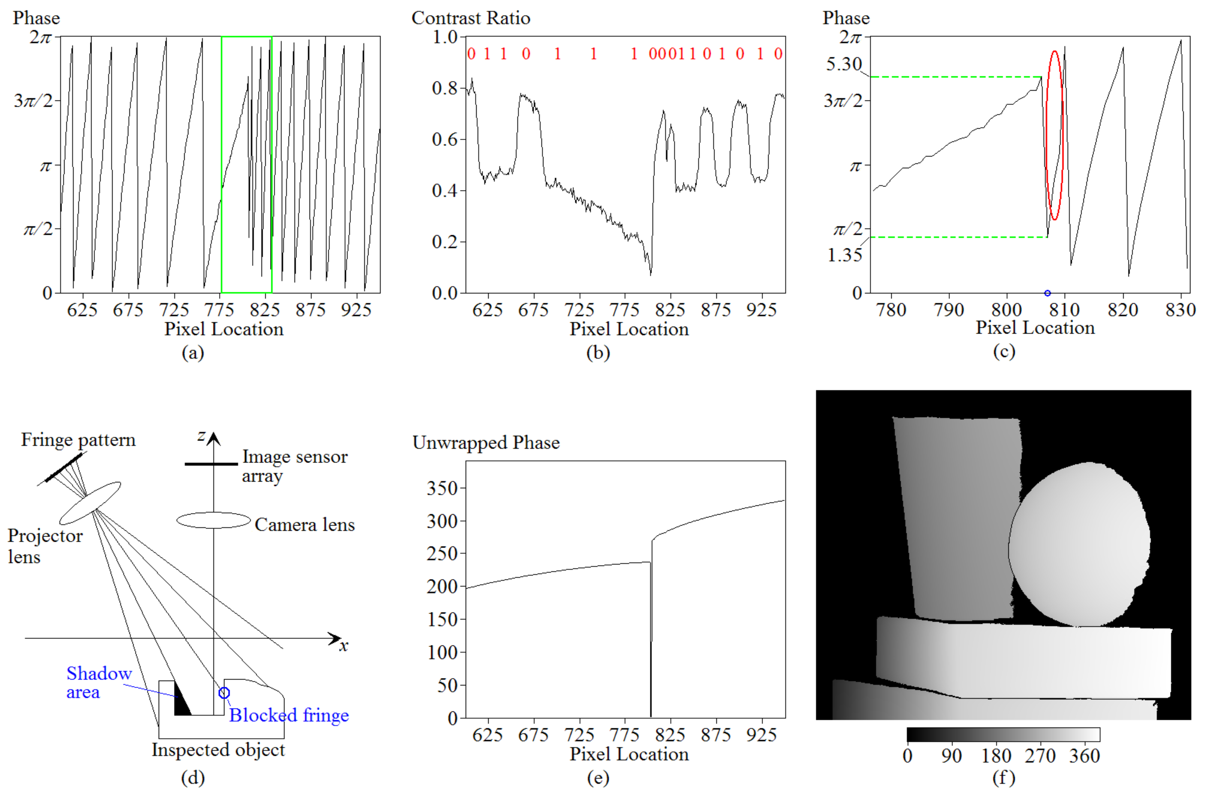
2.4. Correspondences between the Absolute Phase Map and the Surface Profile

It was shown that the position of a surface point in the (x, y, z) coordinates observed by a image pixel (x_d, y_d) can be retrieved from the absolute phase φ(x_d, y_d), as given by [5]

$$z(x_d,y_d)={\displaystyle \sum _{j=1}^J{c}_j{\varphi }^j}(x_d,y_d),$$

(15)

$$x(x_d,y_d)={\displaystyle \sum _{j=0}^1{a}_j{z}^j(x_d,y_d)},$$

(16)

$$y(x_d,y_d)={\displaystyle \sum _{j=0}^1{b}_j{z}^j(x_d,y_d)},$$

(17)

where J is an integer number larger than 1, and a_j, b_j, and c_j are polynomial coefficients. Our previous works presented a calibration scheme [6] to identify these coefficients.

3. Results

3.1. Calibrations

Although the calibration scheme to identify the coefficients expressed in Equation (15) was presented in [5,6], it is necessary to describe the change caused by the fringe encoding. Figure 6a illustrates the optical configuration that was used to identify the coefficients c_j in Equation (15). A 300 mm × 300 mm flat plate with a roughness of approximately 5 microns was selected as the calibration tool. This plate was located in the x–y plane and could be moved along the z-axis with a translation stage. The binary-encoded patterns whose 1D gray-level distributions are shown in Figure 3 were projected onto the calibration tool by the digital projector (Epson EB-U04, with a resolution of 1920 × 1200). The five pattern projections on the calibration tool were sequentially observed by the 12-bit CCD camera (PCO pixelfly qe, with a resolution of 1392 × 1024). The angle between the projector and camera axes shown in Figure 6a was θ = 45°. Figure 6b shows a photo of the setup. Using Equations (6)–(8), distributions of the fringe contrast and phase were extracted. As an example, an image recorded by the CCD camera for the fourth pattern projection (i.e., k = 4) is shown in Figure 6c in which the inspected area was approximately 250 mm × 250 mm and the number of sampling pixels was 1024 × 1024. The 1D distribution along the image row marked with a green frame is shown in Figure 6d. Figure 6e,f respectively shows the extracted phase and contrast distributions for the image row marked with a red frame. As shown in Figure 4a, the contrast distribution at the boundary between the “0” and “1” fringes was discontinuous. However, as shown in the circled regions in Figure 6f, the measured distribution at the boundary areas was no longer discontinuous. Meanwhile, as shown in Figure 6e, slight fluctuations in the circled areas were observed. The reason was the diffraction and lens aberrations caused the point spread function [27] to spread for many pixels.

The convolution of the input signal I_p and the point spread function caused the observed gray levels I_d at the boundary between the “0” and “1” fringes to be smeared by neighbor pixels. Hence, the gray-level distribution was no longer discontinuous. Evidence can be found at the circled areas shown in Figure 3 in which the gray-level distributions were discontinuous at the boundaries between the “0” and “1” fringes. The corresponding output distributions became continuous, as shown in the circled areas in Figure 6d. The linearity illustrated in Figure 5c was inaccurate in the boundary area, leading to errors in employing Equations (6) and (7) to extract the fringe contrasts. The contrast distribution in the circled regions in Figure 6f became continuous. For the same reason, the nonlinearity produced errors when using Equation (8), resulting in a fluctuation in the distribution of wrapped phases.

For a flat surface without any textures and depth discontinuities, there are a couple of methods available to perform the task of phase unwrapping. In this calibration scheme, unwrapping was performed with Goldstein’s method [28].

The task of phase extraction and unwrapping was repeated as the plate was positioned at various depth positions (i.e., z = z₀, z₁, …, z_i). Hence, a phase-to-depth correspondence for each image pixel was obtained. The correspondence between the contrasts and depth positions for each pixel was identified as well. Figure 7a,b illustrates such correspondences for one selected pixel. To provide a close-up view, only the depth position ranging from 0.0 mm to 13.0 mm is plotted. Two boundaries between the “0” and “1” fringes were observed by the image pixel as the flat plate was moved to z = 3.0 mm and 9.6 mm, respectively. Hence, the phase-to-depth correspondence fluctuated in the circled areas shown in Figure 7a. Meanwhile, a change in contrast was observed in the same depth regions, as shown in Figure 7b.

With the phase-to-depth correspondence, the depth position could be represented as a polynomial function of the phase. Then, coefficients c_j could be carried out using a curve-fitting process.

To identify the coefficients expressed in Equation (16), a 1D sinusoidal fringe pattern located in the x–y plane was used as the calibration tool. As shown in Figure 8a, this pattern was mounted on the translation stage and could be moved along the z-axis. Its fringes were parallel to the x-axis, and the period of fringes T_x was a known value. The 12-bit CCD camera (PCO pixelfly qe) was employed to observe this fringe pattern. Figure 8b shows a photo of the experimental setup. The phase of the sinusoidal pattern observed by the camera was extracted using the Fourier transform method [29]. Unwrapping was then performed with Goldstein’s method [28]. The task of measuring the phase was repeated at various depth positions. Hence, a correspondence between the unwrapped phase φ_x and the depth position z for each image pixel was obtained. Given that φ_x can be expressed in terms of x (i.e., φ_x = 2πx/T_x), such a correspondence can be translated to a relationship between x and z. Figure 8c shows the z-to-x relationship for one selected image pixel. Consequently, the coefficients described in Equation (16) could be identified with a subsequent fitting process. In the same way, with a sinusoidal pattern in which its fringes were parallel to the y-axis, the coefficients in Equation (17) could be calculated.

3.2. Systematic Accuracy

To evaluate the accuracy of the profile measurements, a 30 mm × 42 mm standard gauge block with a roughness of approximately 2 μm was selected as the inspected object. Figure 9a shows a recorded image for the first pattern projection (i.e., k = 1) on the inspected object. Figure 9d shows the 1D distribution along one selected image row. Using Equations (6)–(8), the wrapped phase map φ_w(x_d, y_d,) and the contrast map C_d(x_d, y_d,) could be found. Figure 9b,c shows the extracted phase and contrast maps, respectively. Their distributions along one image row are shown in Figure 9e,f, respectively.

The local maxima illustrated in Figure 9d were higher than the gray level of 1130. As described in Section 2.2, it can be categorized into the case of high-reflectance surfaces. Consequently, both Equations (11) and (12) could be used to decode fringes. Figure 9d shows a stream of binary digits that were computed using Equation (11). The binary stream listed in Figure 9f is obtained by Equation (12). Both the decoded streams could be employed to identify the fringe orders. Using the look-up table shown in Figure 2a, they were found to range from 40 to 48. The unwrapped phase map was then carried out using Equation (14). Figure 9g shows the unwrapped phase map. Its 1D distribution along an image row is illustrated in Figure 9h.

Figure 9i shows a close-up view of Figure 9h. As mentioned in Section 3.1, the observed gray levels were not discontinuous at the boundaries between the “0” and “1” fringes. Hence, the contrast distribution was no longer discontinuous in the circled areas shown in Figure 9f. Phases also fluctuated in the same areas. As illustrated in the marked circles shown in Figure 9i, two fluctuations appeared at φ = 40 × 2π and 42 × 2π, respectively.

Fortunately, such fluctuations could be calibrated. An example is illustrated in Figure 7a, which shows the correspondence between the fluctuated phase and the depth position. Using Equations (15)–(17), the profile of the standard gauge block was retrieved. Figure 10a shows the retrieved profile. Its 1D distribution along the x-axis is shown in Figure 10b. In the low contrast area, the amplitude of the projected fringes was reduced, producing more errors in the retrieved profile. In our measurement system, the depth accuracy at the low contrast area was approximately 300 µm, and that at the high contrast area was approximately 100 µm. The depth accuracy was evaluated as the difference between the local maximum and the local minimum of the depth profile.

As a comparison, a combination of binary-coding and phase-shifting projections [16] were employed to retrieve the profile of the gauge block. Figure 11a,b shows the 1D distributions of the patterns used to perform the five-step phase-shifting technique and to identify the fringe orders, respectively. The sequential projections of the binary patterns shown in Figure 11b formed codewords. The fringe orders were then discerned using the codewords. The total number of sinusoidal fringes was 64. Hence, the number of binary patterns was six (i.e., 2⁶ = 64). Using Equation (14), the absolute phases could be obtained. Again, as described in Equations (15)–(17), the profile was retrieved using the absolute phase. The coefficients in Equations (15)–(17) were identified using the calibration scheme described in [5,6]. Figure 12a shows the retrieved profile. Its 1D profile along the x-axis is shown in Figure 12b. The gray level of the sinusoidal fringes was ranging from 25 to 225, which was the same as the “0”-encoded fringe described in Equation (2). Consequently, the systematic accuracy was similar to that at the area of the “0”-encoded fringes, approximately 100 µm.

3.3. Simulations for Errors Caused by Reducing Fringe Contrasts

It was shown that the standard deviation of the extracted phase values, σ_φ, is inversely proportional to the fringe contrast [30,31]. However, as shown in Equation (3), both the fringe contrast C_m and the DC gray level A_m are quantized into two levels. Such changes might cause σ_φ to be not inversely proportional to C_m. To evaluate the change in systematic accuracy caused by modulating C_m and A_m, a comparative simulation was performed. Figure 13a shows the observed 1D distribution I_d when illuminating a screen with an input gray level I_p = 120. The average of the observed gray levels I_d was 1992.1, and the standard deviation of the white noise was 50.198. The corresponding signal-to-noise ratio (SNR) was approximately 40 (i.e., 1992.1/50.198 ≈ 40). Based on this, a white noise generator with SNR = 40 was produced using the software MATLAB. Figure 13b shows the simulated distribution.

The five single-frequency patterns whose distributions are shown in Figure 11a were used to evaluate the simulation precision. With reference to Equation (2), their corresponding DC bias and fringe contrast were A_m = 125 and C_m = 0.8, respectively. A set of five patterns I_d^(k) was carried out using Equation (4). Figure 14a shows the simulated result to represent the first observed projection I_d⁽¹⁾ by adding white noises with SNR = 40. With Equation (8), the phase of the simulation was extracted. Unwrapping was performed using Goldstein’s method. In the experiment using the combination of binary-coding and phase-shifting projections, the coefficients in Equation (15) were calculated. Hence, the profile could be retrieved from the simulated projections. Figure 14b shows the retrieved profile along one image row. The depth profile’s standard deviation was σ_z = 29.6 µm. The difference between the local maximum and the local minimum was approximately 100 µm, which was similar to the real case.

The simulation was performed for another set of five single-frequency patterns. The maximum gray level of the input patterns was 225, but the minimum was increased to 40. Hence, the corresponding DC gray level and contrast ratio were A_m = 132.5 and C_m = 0.698, respectively. The computed standard deviation of the depth profile was σ_z = 32.3 µm.These kinds of simulations were repeated for sinusoidal patterns with various fringe amplitudes, wherein all the maximum gray levels were 225, but the minimum gray levels were sequentially changed into various values: 55, 70, 85, …, 145, 160, and 175. A list of the standard deviations σ_z for various fringe amplitudes B_m and corresponding DC gray levels A_m is depicted in

Table 1. A list of standard deviations with corresponding fringe amplitudes, DC gray levels, and minimum gray levels.

Standard Deviation of the Depth Profile, σz (µm)	158.0	116.4	94.9	77.3	64.7	56.4	47.0	40.6	37.0	32.3	29.6
Fringe amplitude in Ip(k), Bm	25	32.5	40	47.5	55	62.5	70	77.5	85	92.5	100
DC gray level in Ip(k), Am	200	192.5	185	177.5	170	162.5	155	147.5	140	132.5	125
Minimum gray level in Ip(k), Am − Bm	175	160	145	130	115	100	85	70	55	40	25
Contrast ratio, Cm = Bm/Am	0.13	0.17	0.22	0.27	0.32	0.39	0.45	0.53	0.61	0.70	0.80
Product of σz and Cm	19.75	19.67	20.50	20.72	20.96	21.71	21.24	21.32	22.46	22.55	23.68

. The corresponding minimum gray levels, contrast ratios, and products of σ_z and C_m are listed as well. The product of σ_z and C_m was not constant, indicating that σ_φ or σ_z was not inversely proportional to C_m. The reason was that the DC gray levels changed with the contrast ratios. Data points with a fitted relationship between σ_z and C_m are shown in Figure 15.

3.4. Profile Measurements for Surfaces with Depth Discontinuities and Periodic Textures

To evaluate the performance for surfaces with depth discontinuities and periodic reflectance distributions, the objects shown in Figure 16a were selected as the inspected samples. Figure 16b illustrates the appearance of the first pattern projection (i.e., k = 1) onto the inspected objects. The phase map and contrast map are shown in Figure 16c,d, respectively. Figure 16e–g sequentially illustrates the gray level, phase, and contrast distribution along the image row marked with a red frame in Figure 16b. As shown in Figure 16e, the local maxima were significantly above the threshold of 1130. Hence, they could be categorized as high-reflection surfaces. However, as is marked in the red circle, due to the reduced reflection coefficient, the local maximum was suppressed, causing uncertainties when decoding the fringe using Equation (11). Consequently, fringes were decoded with Equation (12). The decoded digits are listed in Figure 16g.

To identify the fringe orders for surfaces with depth discontinuities, an image row marked with a green frame shown in Figure 16b was used as an example. The phase and contrast distributions along the marked image row are shown in Figure 17a,b, respectively. A stream of binary digits that was decoded using Equation (12) is listed in Figure 17b. Figure 17c shows a close-up view for the frame marked in Figure 17a. By removing the discontinuities caused by 2π jumps, a phase jump located at pixel 807 was found, as marked in the blue circle. The jump value was −3.95. As shown in Figure 17d, due to the tilted projection, obstructions and shadows appeared in the depth-discontinuous area. The obstruction caused the phase to be discontinuous in the depth-discontinuous area. On the other hand, the unwrapped phase distributions were continuous on the depth-continued surfaces. Consequently, the phase jump at pixel location 807 was caused by a depth discontinuity. After removing the discontinuities caused by 2π jumps, finding the location of depth discontinuities became a problem of searching for the location of phase discontinuities. One special case was that the jump value caused by the depth discontinuity was equal to a multiple of 2π, leading to a mistake when trying to identify the depth-discontinuous location. In our experiments, this happened occasionally at a few pixels. Such mistakes could simply be recovered with reference to neighboring image rows. Meanwhile, in the area marked with a red circle shown in Figure 17c, where the pixel locations ranged from 807 to 810, the slope of the phase distribution was so large that the projected fringe was sampled by few pixels. Such data points were removed because they caused inaccuracies when retrieving the profile. The entire image row was then divided into two segments: the left side and right side of the depth discontinuity or null points. The fringe orders were individually identified for each segment. With reference to the look-up table shown in Figure 2a, the fringe orders for each segment were known. They ranged from 33 to 39 for the left-hand segment and from 44 to 53 for the right-hand segment. With Equation (14), the phases were unwrapped. Figure 17e shows the unwrapped phase distribution. The task of unwrapping was repeated one image row by one image row. Figure 17f shows the entire unwrapped phase map. A gray-level bar was attached to address the corresponding phase. Using Equations (15)–(17), the profile was calculated. Figure 18 shows the retrieved profile.

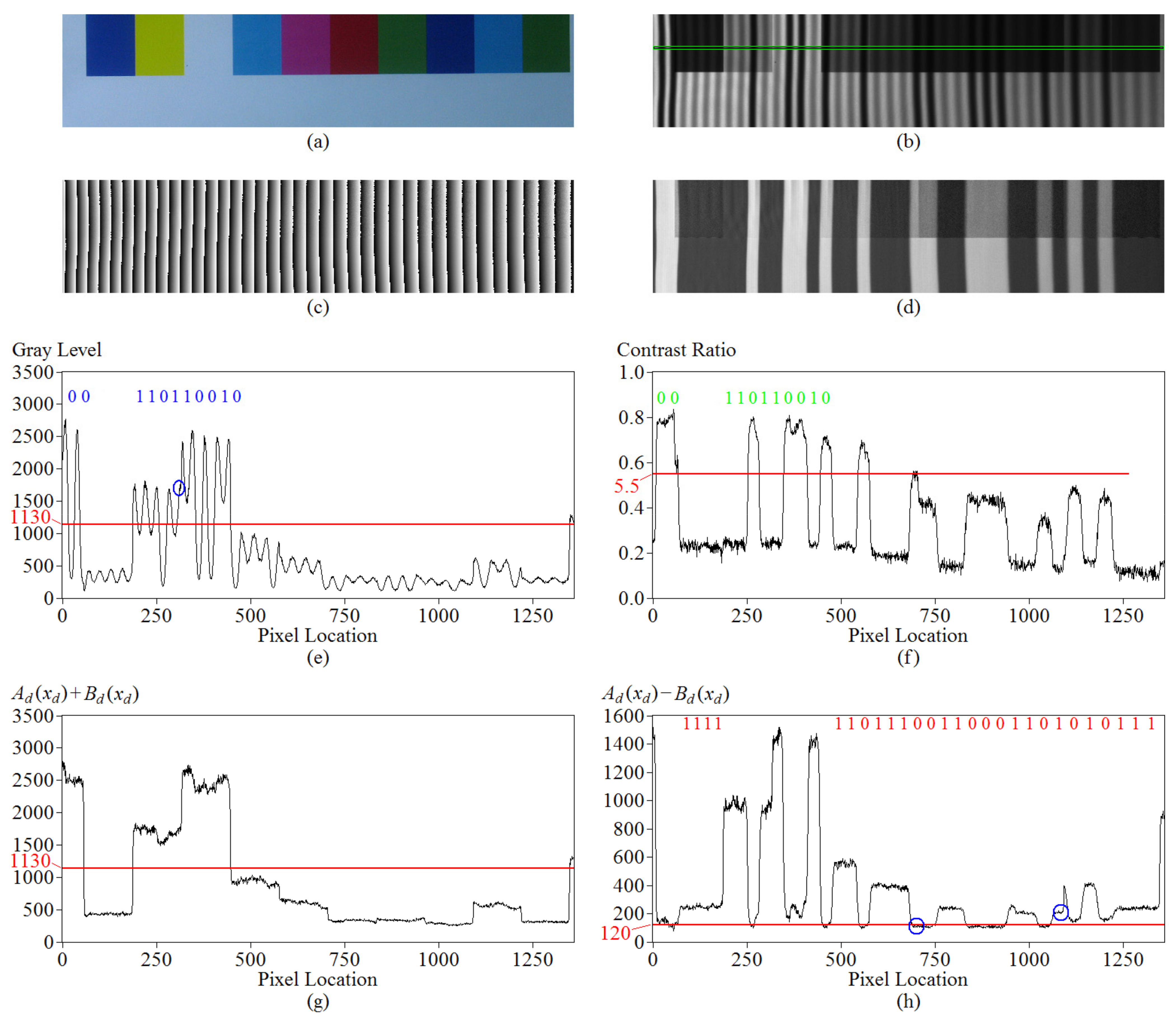
3.5. Fringe Decoding for Reflectance-Discontinuous Surfacesor Surfaces with Low Reflectance Coefficients

A piece of paper that was textured with various colors, as shown in Figure 19a, was chosen as the inspected sample. Figure 19b shows an image that was recorded using the 12-bit CCD camera for the first pattern projection on this surface. The phase and contrast maps that were extracted by the phase-shifting algorithm are illustrated in Figure 19c,d, respectively. Along the image row marked with a green frame that is shown in Figure 19b, the gray-level distribution and contrast distribution are shown in Figure 19e,f, respectively.

A threshold value of 1130 was considered in Figure 19e. The areas where the local maxima were above the threshold were categorized as the cases of high-reflectance surfaces. The method mathematically expressed in Equation (11) was employed to decode the fringes. The decoded digits are listed in Figure 18e. As shown in the circled area, a fringe was mapped to the reflection-discontinuous area. Although the local maxima at two sides of the reflection-discontinuous area were smeared by the surface reflectance, this fringe was decodable. The two local maximum gray levels were not four times larger than the local minimum gray level. Therefore it was decoded as “1”. Meanwhile, the method mathematically expressed in Equation (12) was used to decode fringes for these areas. A stream of binary digits that was obtained using this method is shown in Figure 19f. Both methods were available for high-reflectance surfaces with reflectance discontinuities.

As described in Section 2.3, for areas where the local maximum gray levels were beneath the threshold of 1130, fringes were decoded using Equation (13). Figure 19g,h shows a 1D distribution of A_d + B_d and A_d − B_d, respectively. A list of binary digits that were decoded using Equation (13) is shown in Figure 19h. Locations of the reflectance discontinuities are marked with blue circles. The fringes were decodable for all of the low reflectance surfaces, even though reflection discontinuities appeared. By assembling the binary stream shown in Figure 19e (or Figure 19f) with the stream shown in Figure 19h, all the fringes were decoded.

4. Discussion

To identify the fringe orders for depth-discontinuous surfaces, a method for finding the locations of phase discontinuities was employed. Note that the discontinuities of the absolute phase map can only occur at locations of depth discontinuities. More specifically, with the phase-to-depth relationship shown in Equation (15), the discontinuous depth profile must be retrieved from a discontinuous phase map. Examples are illustrated in Figure 17f and Figure 18. Consequently, the locations of depth discontinuities could be carried out using the discontinuities of the absolute phase map. Based on this, the wrapped phase map (after removing the discontinuities caused by 2π jumps) could be employed to find the locations of the depth discontinuities, except for the cases where the phase jump that was caused by the depth discontinuity was equal to a multiple of 2π. Once the locations of the depth discontinuities were known, fringe orders could be individually identified for each depth-continuous surface. Compared with the method that distinguishes depth discontinuities from the inconsistency in discerning fringe orders [23], it efficiently simplified the unwrapping procedure. However, if the entire depth-discontinuous area presents the same phase jump with a multiple of 2π, then this method cannot work.

The fringe patterns that were used to perform the phase-shifting algorithm were spatially encoded with binary contrast ratios, and the local minima of the first pattern projection were further quantized into two levels. Hence, the projected fringes could be decoded either by means of evaluating the contrast ratios with a threshold or by means of evaluating the fraction of gray levels at φ_w = π and φ_w = 0 (or 2π) for the first pattern projection. For surfaces with low reflection coefficients, an alternate decoding method that uses Equation (13) was presented. The more choices that are available for fringe decoding make it flexible for unwrapping phases of surfaces with complicated textures. The patterns that are used for phase extraction are also employed for unwrapping. Compared with the method that combines the binary-coding and phase-shifting projections to identify the absolute phase map, it reduced the number of pattern projections and the measurement time.

However, it encountered limitations. They are listed as follows.

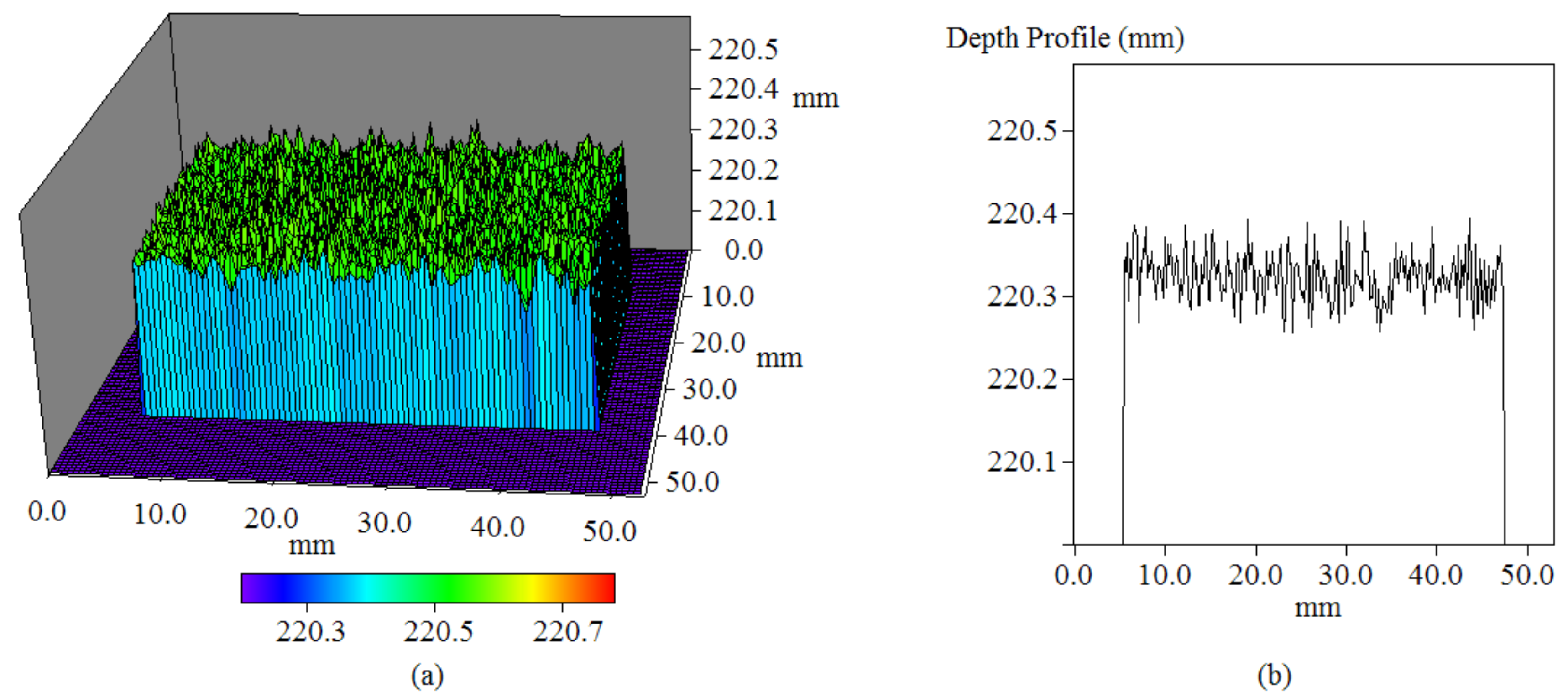
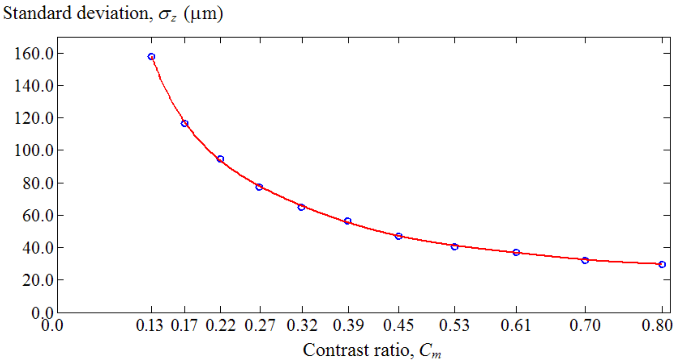
• The reduced contrast produced more noise in the depth profile. A simulated relationship between the standard deviation of the depth profile and the contrast ratio of the input pattern is shown in Figure 15.
• Although the phase and contrast were extracted from the temporal projections, the fringe order was discerned based on spatial encoding schemes. Consequently, it suffered the same challenge as one-shot methods [23]: fringe orders cannot be known when the surface size is so small that the projected fringes cannot form a codeword.
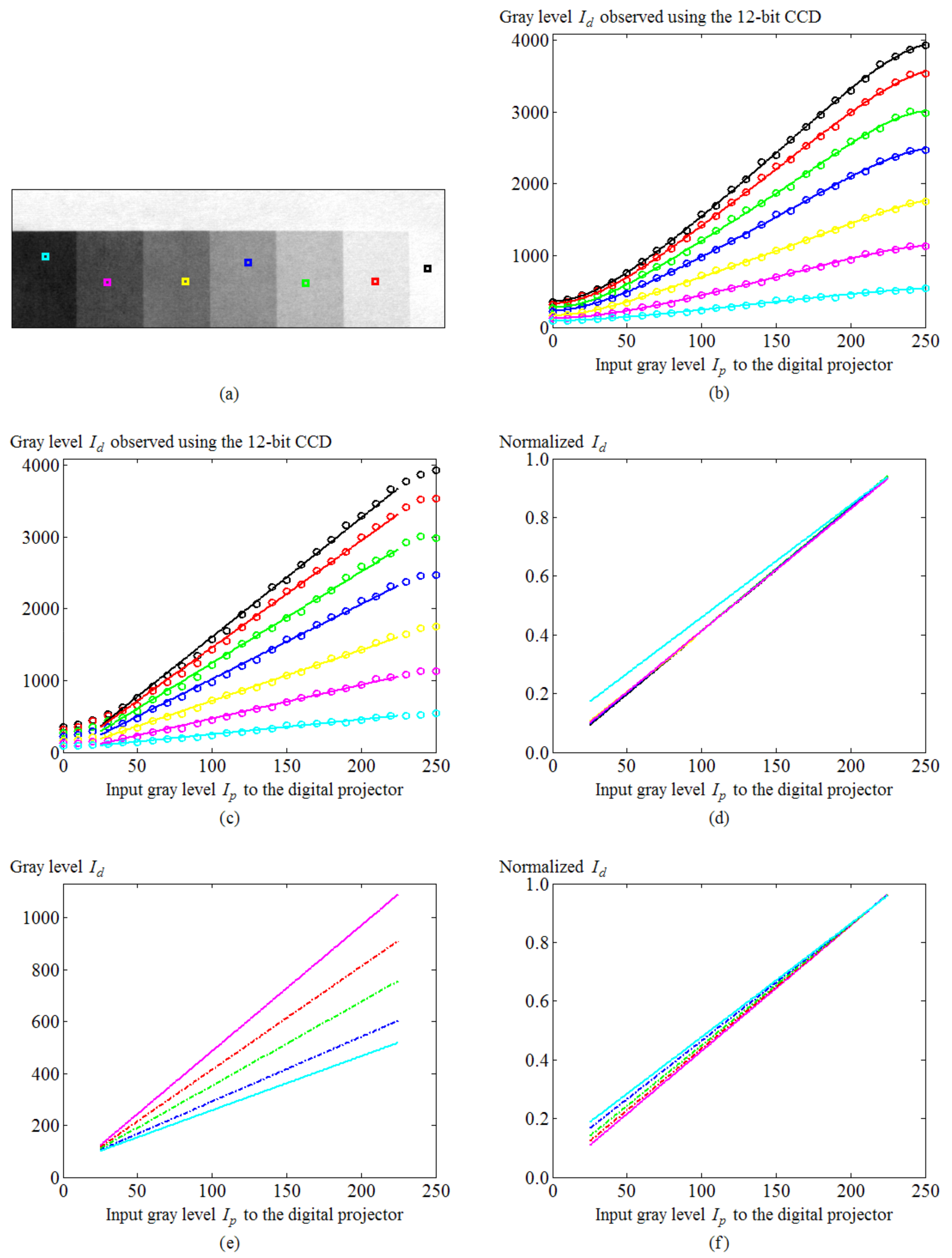
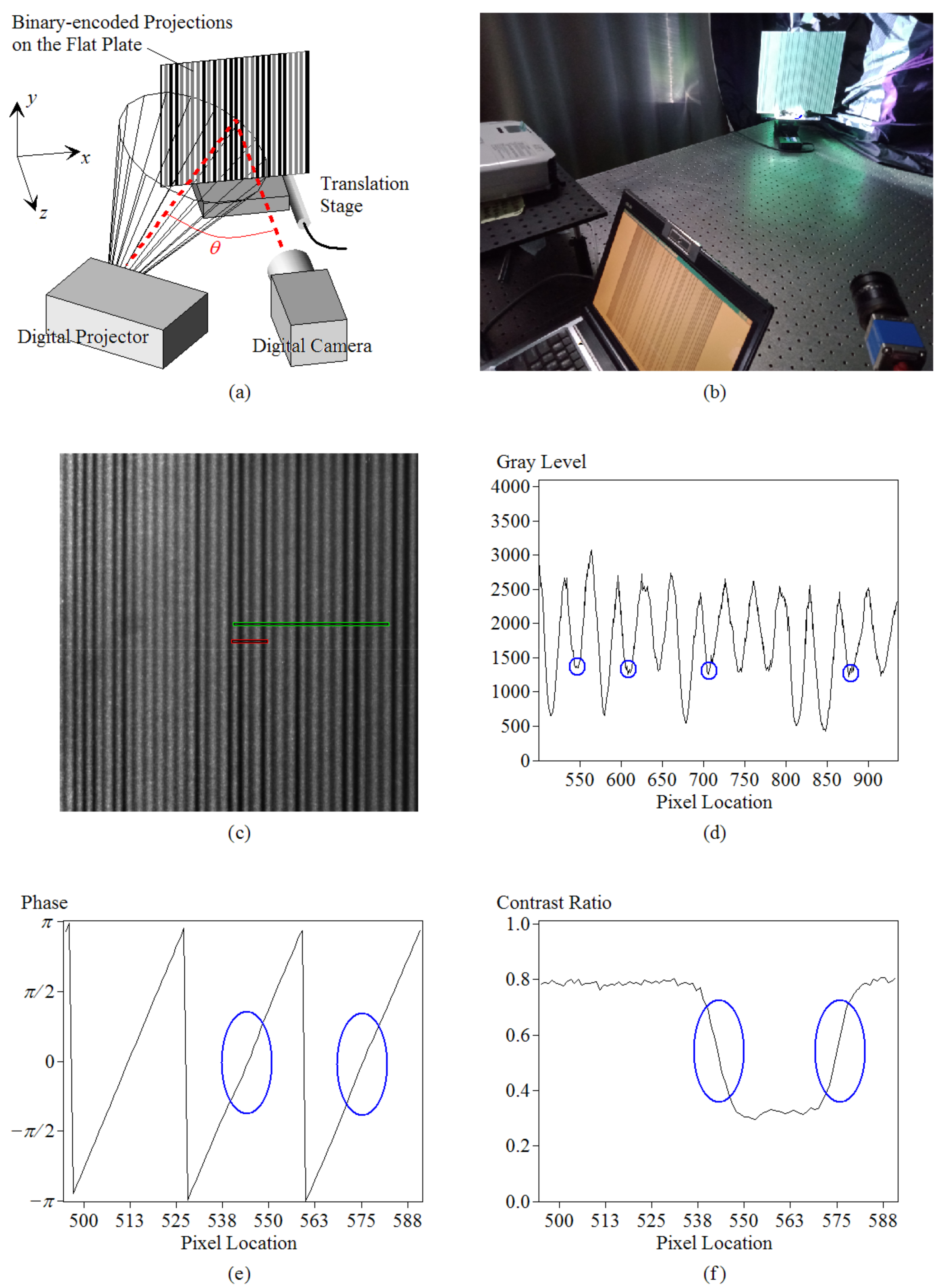
• The measurement system was sensitive to light pollution. Before the profile measurement, calibrations for the relationship between the input gray level and the observed gray level were performed. Such calibrations included identifying the area of linearity illustrated in Figure 5c, defining the gray-level threshold to categorize the surfaces into two cases (i.e., the high reflectance and the low reflectance case), and finding the observed minimum gray level shown in Figure 5e. Then, the profile measurement was performed in the same circumstance, with the same exposure time of the CCD camera and the same size of the lens aperture. Consequently, it was sensitive to light pollution. Unwanted light pollution increased the DC gray level and reduced the contrast ratio. It caused the contrast threshold of 5.5 and the gray-level threshold of 1130 to no longer be available.

5. Conclusions

A set of binary-encoded fringe patterns was presented for phase-shifting fringe projection profilometry. Its performances for surfaces with periodic reflection distributions, surfaces with depth discontinuities, surfaces with reflection discontinuities, and surfaces with low reflection coefficients were discussed. The fringe patterns used for phase extraction could be employed to identify fringe orders directly. Hence, it reduces the number of pattern projections (for phase unwrapping) and the measurement time. The trade-off was that more noise was added to the extracted phase. A simulation for errors caused by reducing the fringe contrasts was provided. A comparison between the presented method and the method combining the binary-coding and phase-shifting projections was provided as well. For a field of view 250 mm × 250 mm, the accuracy of the retrieved profile was approximately 100 µm in the high-contrast area and 300 µm in the low-contrast area. Aside from the increased noise, its other limitations were its inability to know the fringe orders of small surfaces and its sensitivity to light pollution.

References

1. Srinivasan, V.; Liu, H.C.; Halioua, M. Automated phase-measuring profilometry of 3-D diffuse objects. Appl. Opt. 1984, 23, 3105–3108. [Google Scholar] [CrossRef] [PubMed]
2. Larkin, K.G.; Oreb, B.F. Design and assessment of symmetrical phase-shifting algorithms. J. Opt. Soc. Am. A 1992, 9, 1740–1748. [Google Scholar] [CrossRef] [Green Version]
3. Su, X.-Y.; Von Bally, G.; Vukicevic, D. Phase-stepping grating profilometry: Utilization of intensity modulation analysis in complex objects evaluation. Opt. Commun. 1993, 98, 141–150. [Google Scholar] [CrossRef]
4. Liu, H.; Su, W.-H.; Reichard, K.; Yin, S. Calibration-based phase-shifting projected fringe profilometry for accurate absolute 3D surface profile measurement. Opt. Commun. 2003, 216, 65–80. [Google Scholar] [CrossRef]
5. Su, W.H.; Liu, H.; Reichard, K.; Yin, S.; Yu, F.T.S. Fabrication of digital sinusoidal gratings and precisely conytolled diffusive flats and their application to highly accurate projected fringe profilometry. Opt. Eng. 2003, 42, 1730–1740. [Google Scholar] [CrossRef]
6. Creath, K. Step height measurement using two-wavelength phase-shifting interferometry. Appl. Opt. 1987, 26, 2810–2816. [Google Scholar] [CrossRef]
7. Huntley, J.M.; Saldner, H.O. Temporal phase-unwrapping algorithm for automated inteferogram analysis. Appl. Opt. 1993, 32, 3047–3052. [Google Scholar] [CrossRef]
8. Zhao, H.; Chen, W.; Tan, Y. Phase-unwrapping algorithm for the measurement of three-dimensional object shapes. Appl. Opt. 1994, 33, 4497–4500. [Google Scholar] [CrossRef]
9. Saldner, H.O.; Huntley, J.M. Temporal phase unwrapping: Application to surface profiling of discontinuous objects. Appl. Opt. 1997, 36, 2770–2775. [Google Scholar] [CrossRef]
10. Hao, Y.; Zhao, Y.; Li, D. Multifrequency grating projection profilometry based on the nonlinear excess fraction method. Appl. Opt. 1999, 38, 4106–4110. [Google Scholar] [CrossRef]
11. Li, E.B.; Peng, X.; Xi, J.; Chicharo, J.F.; Yao, J.Q.; Zhang, D.W. Multi-frequency and multiple phase-shift sinusoidal fringe projection for 3D profilometry. Opt. Express 2005, 13, 1561–1569. [Google Scholar] [CrossRef]
12. Geng, J. Structured-light 3D surface imaging: A tutorial. Adv. Opt. Photon. 2011, 3, 128–160. [Google Scholar] [CrossRef]
13. Minou, M.; Kanade, T.; Sakai, T. A method of time-coded parallel planes of light for depth measurement. Trans. IECE Jpn. 1981, 64, 521–528. [Google Scholar]
14. Sansoni, G.; Corini, S.; Lazzari, S.; Rodella, R.; Docchio, F. Three-dimensional imaging based on Gray-code light projection: Characterization of the measuring algorithm and development of a measuring system for industrial applications. Appl. Opt. 1997, 36, 4463–4472. [Google Scholar] [CrossRef] [Green Version]
15. Brenner, C.; Boehm, J.; Guehring, J. Photogrammetric calibration and accuracy evaluation of a cross-pattern stripe projector. Proc. SPIE 1998, 3641, 164–172. [Google Scholar] [CrossRef]
16. Sansoni, G.; Carocci, M.; Rodella, R. Three-dimensional vision based on a combination of gray-code and phase-shift light pro-jection: Analysis and compensation of the systematic errors. Appl. Opt. 1999, 38, 6565–6573. [Google Scholar] [CrossRef] [PubMed] [Green Version]
17. Wang, Y.; Zhang, S. Novel phase-coding method for absolute phase retrieval. Opt. Lett. 2012, 37, 2067–2069. [Google Scholar] [CrossRef]
18. Zheng, D.; Da, F. Phase coding method for absolute phase retrieval with a large number of codewords. Opt. Express 2012, 20, 24139–24150. [Google Scholar] [CrossRef] [PubMed]
19. Chen, X.; Wang, Y.; Wang, Y.; Ma, M.; Zeng, C. Quantized phase coding and connected region labeling for absolute phase retrieval. Opt. Express 2016, 24, 28613–28624. [Google Scholar] [CrossRef]
20. Boyer, K.L.; Kak, A.C. Color-Encoded Structured Light for Rapid Active Ranging. IEEE Trans. Pattern Anal. Mach. Intell. 1987, 9, 14–28. [Google Scholar] [CrossRef]
21. Su, W.-H. Color-encoded fringe projection for 3D shape measurements. Opt. Express 2007, 15, 13167–13181. [Google Scholar] [CrossRef]
22. Su, W.-H. Projected fringe profilometry using the area-encoded algorithm for spatially isolated and dynamic objects. Opt. Express 2008, 16, 2590–2596. [Google Scholar] [CrossRef]
23. Su, W.-H.; Chen, S.-Y. One-shot profile inspection for surfaces with depth, color and reflectivity discontinuities. Opt. Express 2017, 25, 9999. [Google Scholar] [CrossRef]
24. Guo, H.; He, H.; Chen, M. Gamma correction for digital fringe projection profilometry. Appl. Opt. 2004, 43, 2906–2914. [Google Scholar] [CrossRef]
25. Liu, K.; Wang, Y.; Lau, D.L.; Hao, Q.; Hassebrook, L.G. Gamma model and its analysis for phase measuring profilometry. J. Opt. Soc. Am. A 2010, 27, 553–562. [Google Scholar] [CrossRef]
26. Li, Z.; Li, Y.F. Gamma-distorted fringe image modeling and accurate gamma correction for fast phase measuring profilometry. Opt. Lett. 2011, 36, 154–156. [Google Scholar] [CrossRef] [PubMed]
27. Goodman, J.W. Introduction to Fourier Optics, 3rd ed.; Roberts & Company: Englewood, CO, USA, 2005; pp. 138–140. [Google Scholar]
28. Zappa, E.; Busca, G. Comparison of eight unwrapping algorithms applied to Fourier-transform profilometry. Opt. Lasers Eng. 2008, 46, 106–116. [Google Scholar] [CrossRef]
29. Takeda, M.; Mutoh, K. Fourier transform profilometry for the automatic measurement of 3-D object shapes. Appl. Opt. 1983, 22, 3977–3982. [Google Scholar] [CrossRef]
30. Brophy, C.P. Effect of intensity error correlation on the computed phase of phase-shifting interferometry. J. Opt. Soc. Am. A 1990, 7, 537–541. [Google Scholar] [CrossRef]
31. Fischer, M.; Petz, M.; Tutsch, R. Statistical characterization of evaluation strategies for fringe projection systems by means of a model-based noise prediction. J. Sens. Sens. Syst. 2017, 6, 145–153. [Google Scholar] [CrossRef] [Green Version]
Figure 1. Optical configuration of phase-shifting fringe projection profilometry.
Photonics 08 00362 g001
Figure 2. (a) A list of the fringe order n with the corresponding binary digit m. (b) An illustration depicting that the stream of binary digits was formed by assembling 64 codewords.
Photonics 08 00362 g002
Figure 3. One-dimensional gray-level distributions of the five encoded patterns.
Photonics 08 00362 g003
Figure 4. (a) The 1D contrast distributions of the five encoded patterns. (b) The 1D phase distribution of the five encoded patterns wrapped in the interval (0, 2π].
Photonics 08 00362 g004
Figure 5. (a) A piece of paper textured with various reflection coefficients, in which a couple of pixels framed with various colors were selected as the inspected samples. (b) Data points and fitted curves depicting the correspondences between the input gray levels and the observed gray levels for various sampled pixels, wherein the correspondences are plotted as the same colors as the framed pixels shown in (b). (c) Fitted lines for various sampled pixels in the linear area. (d) Fitted relationships between the normalized Ip and input gray levels Id in the linear area. (e) A close-up view of the linear relationships sampled at the magenta-framed pixel and some other noisy pixels. (f) Relationships between the normalized Ip and input gray levels Id.
Photonics 08 00362 g005
Figure 6. (a) An optical configuration for the phase-to-depth calibration. (b) A photo illustrating the experimental setup (c) An image recorded by the CCD camera for the 4th pattern projection on the flat plate. (d) A 1D gray-level distribution for the image row marked with a green frame. (e) Extracted phase distribution for the sampled image row marked with a red frame. (f) Extracted contrast distribution for the same image row in (e).
Photonics 08 00362 g006
Figure 7. (a) A correspondence between the unwrapped phase and the depth position for one selected image pixel. (b) Correspondence between the fringe contrast and the depth position (for the same image pixel).
Photonics 08 00362 g007
Figure 8. (a) An optical configuration for lateral calibrations. (b) A photo illustrating the experimental setup. (c) A correspondence between x and z for a selected image pixel.
Photonics 08 00362 g008
Figure 9. (a) A photo that was recorded using the CCD camera for the first pattern projection on the standard block. (b) The phase map that was extracted using the 5-step phase-shifting algorithm. (c) The contrast map (extracted using the 5-step phase-shifting algorithm). (d) The gray-level distribution along one image row. (e) The phase distribution along the sampled image row. (f) The corresponding 1D contrast distribution. (g) The phase map that was unwrapped using codewords. (h) The unwrapped phase distribution along the sampled image row. (i) A close-up view of the distribution shown in (h).
Photonics 08 00362 g009
Figure 10. (a) The retrieved profile. (b) One-dimensional profile distribution along the x-axis.
Photonics 08 00362 g010
Figure 11. (a) The 1D gray-level distributions of the five sinusoidal patterns. (b) The 1D gray-level distributions of the six binary patterns.
Photonics 08 00362 g011
Figure 12. (a) The profile that was retrieved by means of combining binary-coding and phase-shifting projections. (b) One-dimensional profile distribution along the x-axis.
Photonics 08 00362 g012
Figure 13. (a) The 1D distribution of Id when illuminating a screen with an input gray level Ip = 120. (b) Simulated 1D distribution.
Photonics 08 00362 g013
Figure 14. (a) Simulated 1D distribution for the first sinusoidal projection by adding white noises with SNR = 40. (b) Retrieved 1D profile from the simulated fringe patterns.
Photonics 08 00362 g014
Figure 15. Relationship between the standard deviation of the depth profile and the input fringe contrast.
Photonics 08 00362 g015
Figure 16. (a) An appearance of the inspected objects. (b) An image that was obtained from the first pattern projection on the objects. (c) The extracted phase map. (d) The contrast map. (e) The gray-level distribution along the image row that is marked with a red frame in (b). (f) The corresponding 1D phase distribution. (g) The corresponding 1D contrast distribution.
Photonics 08 00362 g016
Figure 17. (a) The phase distribution along the image row that is marked with a green frame in Figure 16b. (b) The corresponding contrast distribution. (c) A close-up view of the green frame that is marked in (a). (d) A configuration illustrating obstructions and shadows caused by tilted projections. (e) The unwrapped phase distribution along the sampled image row. (f) The entire unwrapped phase map.
Photonics 08 00362 g017
Figure 18. (a) The retrieved profile. (b) The retrieved profile as observed from another view angle.
Photonics 08 00362 g018
Figure 19. (a) An appearance of the inspected surface that was textured with various colors. (b) The recorded image for the first pattern projection on the inspected object. (c) The extracted phase map. (d) The extracted contrast map. (e) The gray-level distribution along the image row that is marked with the green frame shown in (b). (f) The corresponding 1D contrast distribution. (g) 1D distribution of Ad(xd, yd) + Bd(xd, yd) along the marked image row. (h) 1D distribution of Ad(xd, yd) − Bd(xd, yd) along the marked image row.
Photonics 08 00362 g019