Review

Two-Membrane Cavity Optomechanics: Linear and Non-Linear Dynamics

by
Paolo Piergentili
1,2,*,
Riccardo Natali
1,2,
David Vitali
1,2,3 and
Giovanni Di Giuseppe
1,2
1
School of Science and Technology, Physics Division, University of Camerino, I-62032 Camerino, Italy
2
Istituto Nazionale di Fisica Nucleare (INFN), Sezione di Perugia, I-06123 Perugia, Italy
3
CNR-INO, L.go Enrico Fermi 6, I-50125 Firenze, Italy
*
Author to whom correspondence should be addressed.
Photonics 2022, 9(2), 99; https://doi.org/10.3390/photonics9020099
Submission received: 21 January 2022 / Revised: 4 February 2022 / Accepted: 5 February 2022 / Published: 8 February 2022
(This article belongs to the Special Issue Optomechanics: Science and Applications)

Abstract

:
In this paper, we review the linear and non-linear dynamics of an optomechanical system made of a two-membrane etalon in a high-finesse Fabry–Pérot cavity. This two-membrane setup has the capacity to modify on demand the single-photon optomechanical coupling, and in the linearized interaction regime to cool simultaneously two mechanical oscillators. It is a promising platform for realizing cavity optomechanics with multiple resonators. In the non-linear regime, an analytical approach based on slowly varying amplitude equations allows us to derive a consistent and full characterization of the non-linear displacement detection, enabling a truthful detection of membrane displacements much above the usual linear sensing limited by the cavity linewidth. Such a high quality system also shows a pre-synchronization regime.

1. Introduction

Cooperative effects, enhanced interactions and nontrivial dynamics occur when multiple mechanical resonators are placed within an optical cavity [1,2,3,4,5,6,7,8,9,10]; for example, one can induce and control the coherent exchange of excitations [11,12,13,14], or study self-oscillations and their synchronization in the case of two or more mechanical resonators [12,15,16,17,18,19,20,21,22,23,24]. In this paper, we review the linear and non-linear dynamics of an optomechanical system made of a two-membrane etalon in a high-finesse Fabry–Pérot cavity [8,10,23]. When the optical cavity is driven on the red sideband, the linear dynamics of such a system is explored: the optomechanical coupling can be controlled on demand [8,9,25] by a local control of the membrane position along the cavity axis, and multiple oscillators can be simultaneously cooled [8,26], or exploited for photon-mediated coherent interaction and heat transfer between separate resonators [13,14]. However, the radiation pressure interaction is proportional to the photon number and it may have non-linear effects on both the mechanical and optical degrees of freedom which become evident when the mechanical motion is excited [27] by means of laser driving on the blue sideband of the optical cavity. Optical backaction in this case counteracts the internal mechanical friction, and when the total effective damping becomes equal to zero, a Hopf bifurcation into a regime of self-induced mechanical oscillations takes place [23,28,29,30,31,32,33,34]. A fixed amplitude limit cycle is established, with a free running oscillation phase, which may lock to external forces or to other optomechanical oscillators [35], leading to synchronization (see references [12,15,16,22,36,37,38,39,40,41,42] for theoretical characterizations, and references [17,18,19,20,21,24,43,44,45,46] for experimental demonstrations in optomechanical and electromechanical devices). In the specific case of the two-membrane-in-the-middle setup of interest here, self-organized synchronization, phase-locking, and the transition between in-phase and antiphase regimes have been qualitatively demonstrated [24], without calibration of the mechanical displacements. An alternative way of describing the non-linear optomechanical dynamics in this mechanical parametric oscillation regime is that the modulation of the radiation pressure interaction induced by the mechanical motion causes a cavity frequency shift comparable to or larger than the optical linewidth, yielding a nontrivial modification of the cavity response.
In this review article we first focus on studying the dynamics of the linearized fluctuations around the stable stationary state of the system, showing the tunability of the single-photon optomechanical coupling rate, and also that both membranes of the etalon can be simultaneously cooled by means of a red-detuned cavity driving. Later on we explore a regime, which can be called pre-synchronization regime, obtained when the blue-detuned driving is weak and slightly below the synchronization threshold. In this regime only one of the two membrane resonators, “master”, is driven to a limit cycle through the Hopf bifurcation, while the other oscillator is only partially synchronized with the “master” resonator because the amplitude of the synchronized component does not prevail over the thermal motion. We show that when multiple mechanical resonators are detected by the same single probe field simultaneously interacting with all of them (such as, for example, in references [17,18,19,43,45]), and at least one resonator enters a limit cycle, one has a non-trivial, non-linear dynamics of the system, which has to be properly considered, yielding a highly non-linear calibration of the displacement measurement obtained by means of the output probe readout.
This review article is organized as follows: in Section 2 we briefly describe the multimode optomechanical system under study, exploring both the linearized dynamics of the fluctuation within the stability conditions, and the non-linear regime, which is obtained when the Hopf bifurcation is crossed, and one has mechanical self-oscillations. In Section 3 we describe the experimental setup, and in Section 4 we present the linear dynamics for the membrane resonators, in particular their controllable coupling and the possibility to cool both of them. In Section 5 we analyze the non-linear dynamics of the mechanical modes at the onset of synchronization, and we provide the analytical recipe able to describe in a quantitative way both the full numerical solution of the Langevin equations, and the experimental results for the optical probe spectrum. Section 6 is for concluding remarks.

2. Theoretical Description of the System Dynamics

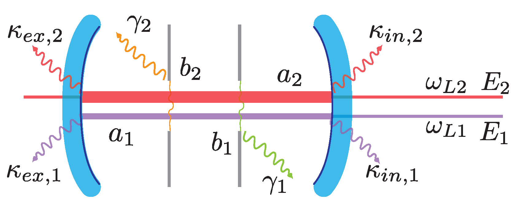
The following Hamiltonian describes an optomechanical system where two optical modes interact with two mechanical modes via radiation pressure:
H = H pump + H probe + H mech + H int ,
decomposed as follows:
H pump = ω c 1 a 1 a 1 + i E 1 a 1 e i ω L 1 t a 1 e i ω L 1 t ,
H probe = ω c 2 a 2 a 2 + i E 2 a 2 e i ω L 2 t a 2 e i ω L 2 t ,
H mech = j = 1 , 2 ω j b j b j ,
H int = i , j = 1 , 2 g i j a i a i ( b j + b j ) .
Two cavity modes with resonance frequencies, ω c 1 and ω c 2 , described by two bosonic annihilation operators a 1 , and a 2 , are driven at frequencies ω L 1 , and ω L 2 , respectively. The mode a 1 , called PUMP, is used for engineering the optomechanical interaction, while a 2 , denominated PROBE, performs a continuous detection of the mechanical motion. To prevent any interference between the two drivings they usually have a different cavity mode from each other (different polarization or frequency). E i = 2 κ i n , i P i / ω L i includes the driving dissipation rates, with κ i n , i the decay rate of the i-th cavity mode through the input mirror, and P i the corresponding laser power.
The Hamiltonian H mech describes two membrane oscillators with bosonic annihilation mechanical operator b j ( j = 1 , 2 ), each with mass m j and resonance frequency ω j , and displacement q j = ( b j + b j ) x zpf , j , where x zpf , j = ( / 2 ω j m j ) 1 / 2 is the zero point motion of the j-th oscillator. The radiation pressure dispersive interaction couples the mechanical modes with the probe and pump optical modes. The single-photon coupling rates g i j = ( d ω c i / d x j ) x zpf , j quantify the optomechanical interaction (see Figure 1).
We consider for both probe and pump modes, the frame rotating at the corresponding laser driving frequency. Fluctuation–dissipation processes couple the cavity modes and the resonators to their related thermal reservoir at temperature T, and they are included in the Heisenberg picture adding noise and dissipative terms. The quantum Langevin equations [27,47,48], for i , j = 1 , 2 , are:
a i ˙ = ( i Δ i ( 0 ) κ i ) a i + E i + i j = 1 , 2 g i j ( b j + b j ) a i + 2 κ i n , i a i n , i + 2 κ e x , i a e x , i ,
b j ˙ = ( γ j i ω j ) b j + i i = 1 , 2 g i j a i a i + 2 γ j b j i n ,
where Δ i ( 0 ) = ω c i ω L i , κ i = κ i n , i + κ e x , i represents the amplitude decay rate of the cavity for the pump and the probe modes, κ e x , i is the optical loss rate through all the ports different from the input one, and γ j represents the amplitude decay rate of the j-th oscillator. a i n , i ( t ) , a e x , i ( t ) and b j i n are the corresponding zero-mean noise reservoir operators. They are all Gaussian, and white noises uncorrelated from each other with correlation functions f ( t ) f ( t ) = n ¯ δ ( t t ) and f ( t ) f ( t ) = ( n ¯ + 1 ) δ ( t t ) where f ( t ) is either a i n , i ( t ) , a e x , i ( t ) or b j i n , and n ¯ = [ exp ( ω f / k b T ) 1 ] 1 is the mean thermal occupation number for the related mode.
We shall restrict, in this review, to study the dynamics at temperature T 300 K only, when a classical treatment of the above quantum Langevin equations is reasonable. At this temperature a different treatment of mechanical and optical noise terms should be considered: the optical frequencies ω c , i / 2 π 10 14 Hz, so that n ¯ c , i 0 , are dominated by photon shot noise, but for large enough driving powers fluctuations of the intracavity field might occur, due either to vacuum fluctuations or technical laser noise. At mechanical frequencies ω 1 / 2 π ω 2 / 2 π 10 6 Hz, implying n ¯ m , j k b T / ω j 1 , the thermal noise is dominant for the mechanical mode. For this reason, we consider classical complex random noises, β j i n ( t ) , j = 1 , 2 , which replace the mechanical quantum thermal noise b j i n ( t ) , and α i o p t ( t ) , which replace the sum of optical vacuum noises κ i n , i / κ i a i n , i ( t ) + κ e x , i / κ i a e x , i ( t ) , with correlation functions [39,42]
β j i n ( t ) β j i n ( t ) = α i o p t ( t ) α i o p t ( t ) = 0 ,
β j i n ( t ) β j i n , * ( t ) = β j i n , * ( t ) β j i n ( t ) = ( n ¯ m + 1 / 2 ) δ j j δ ( t t ) ,
α i o p t ( t ) α i o p t , * ( t ) = α i o p t , * ( t ) α i o p t ( t ) = ( 1 / 2 ) δ i i δ ( t t ) .
Therefore, the following coupled classical Langevin equations well approximates the set of coupled quantum Langevin equations for the optical and mechanical complex amplitudes α i ( t ) and β j ( t ) [38,39,42],
α ˙ i ( t ) = i Δ i ( 0 ) κ i α i ( t ) + E i + j = 1 , 2 2 i g i j Re [ β j ( t ) ] α i ( t ) + 2 κ i α i o p t ( t ) ,
β ˙ j ( t ) = ( i ω j γ j ) β j ( t ) + i i = 1 , 2 g i j | α i ( t ) | 2 + 2 γ j β j i n ( t ) .
In our case, the quasi-resonant weak probe beam is used only for the detection of the mechanical motion of the oscillators. We are far from the regime where the drivings relative phase can be used to control nonreciprocal effects [49,50].

2.1. Linear Dynamics

It is often useful to introduce the linearized approximate description of Equations (11) and (12). In the following we remove the index 1 when referring to the cavity pump field, that is α 1 α , κ 1 κ . We also ignore the Langevin equation of the weak probe beam, which is in resonance with the optomechanical cavity, and therefore realizes a perfectly non-invasive detection of the mechanical mode, without any backaction, as it occurs in a Michelson interferometer readout [34]. The cavity field and the mechanical mode are split into an average coherent amplitude and a fluctuating term α ( t ) = α 0 + δ α ( t ) and β j ( t ) = β j , 0 + δ β j ( t ) . In the steady state case, the average amplitudes are:
α 0 = E κ + i Δ ( 0 ) j = 1 , 2 g j β 0 , j + β 0 , j * ,
β 0 , j = i g j | α 0 | 2 γ j + i ω j .
Neglecting the second order terms, the fluctuation terms δ α ( t ) and δ β j ( t ) give the following linearized Langevin equations [27,51]:
δ α ˙ ( t ) = i Δ + κ δ α ( t ) + i j = 1 , 2 g j [ δ β j ( t ) + δ β j * ( t ) ] α 0 + 2 κ δ α o p t ( t ) ,
δ β ˙ j ( t ) = ( i ω j + γ j ) δ β j ( t ) + i g j [ α 0 * δ α ( t ) + α 0 δ α * ( t ) ] + 2 γ j β j i n ( t ) ,
where Δ = Δ ( 0 ) j = 1 , 2 g j ( β 0 , j + β 0 , j * ) corresponds to a modification of the cavity detuning, which is the parameter controlled in the experiments. For our purpose, it is easier to solve the linearized Langevin equations in the frequency space:
i ω δ α ˜ ( ω ) = i Δ + κ δ α ˜ ( ω ) + i j = 1 , 2 g j α 0 δ β ˜ j ( ω ) + δ β ˜ j * ( ω ) + 2 κ δ α ˜ o p t ( ω ) ,
i ω δ β ˜ j ( ω ) = ( i ω j + γ j ) δ β ˜ j ( ω ) + i g j α 0 * δ α ˜ ( ω ) + α 0 δ α ˜ * ( ω ) + 2 γ j δ β ˜ j i n ( ω ) ,
where δ β ˜ j ( ω ) = + d t e i ω t δ β j ( t ) and δ α ˜ ( ω ) = + d t e i ω t δ α ( t ) are the Fourier transform of δ β j ( t ) and δ α ( t ) . Performing the calculations, and defining the optical and mechanical susceptibility χ ˜ c ( ω ) = κ + i Δ ω 1 and χ ˜ m , j ( ω ) = γ j + i ω j ω 1 , respectively, we obtain:
χ ˜ c 1 ( ω ) δ α ˜ ( ω ) = i j = 1 , 2 g j α 0 δ β ˜ j ( ω ) + δ β ˜ j * ( ω ) + 2 κ δ α ˜ o p t ( ω ) ,
χ ˜ m , j 1 ( ω ) δ β ˜ j ( ω ) = i g j α 0 * δ α ˜ ( ω ) + α 0 δ α ˜ * ( ω ) + 2 γ j δ β ˜ j i n ( ω ) .
To obtain the modified susceptibility for the mechanical oscillator we solve the previous system of equations inserting Equation (19) into (20). Defining Σ ( ω ) = i | α | 2 χ ˜ c * ( ω ) χ ˜ c ( ω ) , and δ u ˜ j o p t = g j α 0 * δ α ˜ o p t χ ˜ c ( ω ) + α 0 δ α ˜ o p t * χ ˜ c * ( ω ) , we get the linearized Langevin equations for the two mechanical oscillators in the rotating wave approximation, that is neglecting the counter-rotating terms δ β ˜ j * [52], which is valid in the red-detuned and resolved-sideband regime (even moderate):
χ ˜ m , 1 1 + i g 1 2 Σ ( ω ) δ β ˜ 1 ( ω ) = i g 1 g 2 Σ ( ω ) δ β ˜ 2 ( ω ) + i 2 κ δ u ˜ 1 o p t + 2 γ 1 δ β ˜ 1 i n ( ω ) ,
χ ˜ m , 2 1 + i g 2 2 Σ ( ω ) δ β ˜ 2 ( ω ) = i g 1 g 2 Σ ( ω ) δ β ˜ 1 ( ω ) + i 2 κ δ u ˜ 2 o p t + 2 γ 2 δ β ˜ 2 i n ( ω ) .
Neglecting the optical noise terms (high temperature regime), we finally obtain:
χ ˜ m , 1 e f f 1 + Σ 1 ( ω ) Σ 2 ( ω ) χ ˜ m , 2 e f f 1 δ β ˜ 1 ( ω ) 2 γ 1 δ β ˜ 1 i n ( ω ) ,
χ ˜ m , 2 e f f 1 + Σ 1 ( ω ) Σ 2 ( ω ) χ ˜ m , 1 e f f 1 δ β ˜ 2 ( ω ) 2 γ 2 δ β ˜ 2 i n ( ω ) ,
where χ ˜ m , j e f f 1 = χ ˜ m , j 1 + i Σ j ( ω ) , and Σ j ( ω ) = g j 2 Σ ( ω ) . From the previous equations, we can derive the effective susceptibility of the two mechanical oscillators driven by a red detuned pump beam [48]:
χ ˜ m , j e f f = χ ˜ m , j e f f 1 + Σ 1 ( ω ) χ ˜ m , 1 e f f Σ 2 ( ω ) χ ˜ m , 2 e f f .

2.2. Non–Linear Dynamics

In the non-linear regime, the chaotic motion of the two oscillators is not considered, as it occurs at extremely large driving powers which are not physically meaningful for the optomechanical system discussed in this review. We might find the dynamics of the system by considering the slowly varying amplitude equations approach of references [16,22]. After an initial transient regime, each mechanical oscillator sets itself into the following dynamics:
β j ( t ) = β 0 , j + A j ( t ) e i ω ref t ,
where β 0 , j is the approximately constant, static shift of the j-th resonator, A j ( t ) is the corresponding slowly–varying complex amplitudes, and ω ref Δ ω is a reference mechanical frequency, of the order of ω j . Equation (26) implies that we will study the long–time dynamics of the two mechanical resonators in the frame rotating at the fast reference frequency ω ref . Inserting the Equation (26) into the Equation (11), and performing explicitly the integrals one gets:
α i ( t ) = e i ψ i ( t ) 0 t d t e W i ( t t ) [ E i + 2 κ i α i o p t ( t ) ] e i ψ i ( t ) α i E ( t ) + δ α i ( t ) ,
where the intracavity field α i E ( t ) is proportional to the driving rate E i , and δ α i ( t ) is related to the input noise α i o p t ( t ) . We defined the bright complex amplitudes A i b ( t ) = | A i b ( t ) | e i θ i ( t ) = g i j A j ( t ) / g i b with g i b = ( g i 1 2 + g i 2 2 ) 1 / 2 , and W i = i [ Δ i ( 0 ) g i j ( β 0 , j + β 0 , j * ) ] κ i , and ψ i ( t ) = ξ i sin ( ω ref t θ i ) with ξ i = 2 g i b | A i b | / ω ref .
By performing the Jacobi–Anger expansion for the e i ψ i ( t ) factor within the integral [16,30], that is, e i ξ sin ϕ = n J n ( ξ ) e i n ϕ , ( ϕ = ω ref t θ i , and J n is the n-th Bessel function of the first kind), and neglecting a transient decay term, the expression for the intracavity field amplitude α i E ( t ) is:
α i E ( t ) = E i e i ψ i ( t ) n = J n ξ i e i n ( ω ref t θ i ) i n ω ref W i .
For the fluctuation term we have:
δ α i ( t ) = 2 κ i e i ψ i ( t ) 0 t d t e W i ( t t ) α i o p t ( t ) .
We might derive an equation for the unknown quantities A j ( t ) and β 0 , j by inserting these relations into the radiation pressure force term within the Equation (12) for the mechanical motion. Since the intracavity optical fluctuations are negligible, one can approximate at first order the radiation pressure term in δ α i ( t ) ,
i g i j | α i ( t ) | 2 i g i j | α i E ( t ) | 2 + i g i j η i o p t ( t ) ,
where
| α i E ( t ) | 2 = E i 2 n , m = J n ξ i J m ξ i e i ( n m ) ( ω ref t θ i ) ( i n ω ref W i ) ( i m ω ref W i * ) ,
and
η i o p t ( t ) = α i E ( t ) δ α i * ( t ) + α i E , * ( t ) δ α i ( t ) .
Assuming β 0 , j approximately constant, and neglecting all the terms that oscillate faster than ω ref , i.e., keeping only the resonant terms in Equation (31) [ n m = 0 for β 0 , j and n m = 1 for the amplitudes A j ( t ) ], we get
( γ j + i ω j ) β 0 , j = i i = 1 , 2 n = g i j E i 2 J n ξ i 2 ( i n ω ref W i ) ( i n ω ref W i * ) ,
which is an implicit equation for β 0 , j because W i depends upon β 0 , j , and the value of β 0 , j can be obtained numerically. For the slowly varying amplitudes A j ( t ) we get instead:
A ˙ j ( t ) = γ j i Δ ω j A j ( t ) + 2 γ j β j i n ( t ) + i i = 1 , 2 g i j η i o p t ( t ) + + i i = 1 , 2 n = g i j e i θ i E i 2 J n ξ i J n + 1 ξ i [ i n ω ref W i ] [ i ( n + 1 ) ω ref W i * ] ,
where Δ ω j = ω j ω ref , and
Δ i ( 0 ) Δ i = Δ i ( 0 ) j = 1 , 2 g i j ( β 0 , j + β 0 , j * ) ,
correspond to a modification of the cavity detunings, as already explained in the previous Section, so that W i = i Δ i κ i can be regarded as a given parameter when we calculate the amplitude.
Finally, the Equation (34) can be rewritten in a more transparent form by making explicit the equation for each amplitude, and by defining the following regular dimensionless auxiliary functions F i ( | A i b | , κ i , Δ i ) , i = 1 , 2 , as:
F i = E i 2 | A i b | n = J n ξ i J n + 1 ξ i [ i n ω ref W i ] [ i ( n + 1 ) ω ref W i * ]
which can be easily shown to be a function of even powers of | A i b | only. One finally gets the set of coupled slowly-varying complex amplitude equations:
A ˙ 1 ( t ) = γ 1 i ( Δ ω 1 d 1 ) A 1 ( t ) + i d 12 A 2 ( t ) + i i = 1 , 2 g i 1 η i o p t ( t ) + 2 γ 1 β 1 i n ( t ) ,
A ˙ 2 ( t ) = γ 2 i ( Δ ω 2 d 2 ) A 2 ( t ) + i d 12 A 1 ( t ) + i i = 1 , 2 g i 2 η i o p t ( t ) + 2 γ 2 β 2 i n ( t ) ,
where
d 1 = g 11 2 F 1 g 1 b + g 21 2 F 2 g 2 b ,
d 2 = g 12 2 F 1 g 1 b + g 22 2 F 2 g 2 b ,
d 12 = g 11 g 12 F 1 g 1 b + g 21 g 22 F 2 g 2 b ,
are non-linear coefficients because of their dependence upon the regular dimensionless auxiliary functions F i , which, in turn, depend upon the corresponding variable | A i b | 2 = | g i 1 A 1 + g i 2 A 2 | 2 / ( g i 1 2 + g i 2 2 ) . As already shown in references [16,22], Equations (37) and (38) give an accurate and general description of two mechanical resonators dynamics.

3. Experimental Setup

In this Section we describe the experimental setup used to study the linear and non-linear dynamics of an optomechanical system constituted of a two-membrane etalon inserted in a high-finesse Fabry–Pérot cavity. The membrane-etalon is realised with two equal 1.5 m m × 1.5 m m membranes (Norcada), with a etalon length L c = 53.571 ( 9 )   μ m . The membranes have a thickness L m = 106 ( 1 )   n m , considering the index of refraction of Si 3 N 4 given in reference [53]. The membrane-sandwich is placed at the center of a high-finesse Fabry–Pérot cavity. Inserting the membrane-etalon, the empty cavity finesse F 0 = 50,125 (25) decreases to F = 12,463 (13), corresponding to an intensity decay rate of the cavity 2 κ = τ 1 = FSR / F 2 π × 134   kHz , with FSR 2 π × 1.67   GHz . The mechanical and optical properties of this system were explored in references [8].
Figure 2 shows the experimental setup. A laser beam at wavelength λ 0 = 1064     n m is split into a pump beam and a probe beam. An acousto-optic modulator (AOM) shifts the frequency of the pump beam by Δ 1 from the cavity resonance. The probe beam is in resonance with the optical cavity and has an intensity P p r o b e = 5.9   μ W . The light reflected by the optical cavity is homodyne detected and the thermal voltage spectral noise (VSN) is measured. The pump beam is used to laser drive the mechanical modes. In the following Sections, we focus on studying the linear and non-linear dynamics with the fundamental modes of the two membranes.

4. Experiments in the Linear Regime

In the linear regime, we first show that shifting the position of the membranes along the cavity axis with the piezo controllers the optomechanical interaction can be tuned and controlled. Figure 3a shows a simulation of the shift of the resonance frequencies of the optomechanical cavity as a function of the position of the two oscillators, q j , along the standing wave resonating in the cavity. The corresponding gradient field is represented as superimposed vector plot, and shows how the two optomechanical couplings G j = ω c a v / q j = g j / x zpf , j change by displacing the membranes [8]. Note that there are positions q j for which only one of the membranes is coupled (red and magenta dots), or both (green dot).
To prove tunability of the optomechanical coupling rate, the probe beam was frequency locked to the optical cavity using the PDH technique, and the thermal VSN of the two membranes is measured with homodyne detection of the light reflected by the optical cavity (see Figure 2). Figure 3b shows the detected thermal VSN, which clearly demonstrates the capacity to switch off and on the optomechanical interaction in a controlled way by shifting the position of each membrane (see Figure 3b top and middle spectra, and also the magenta and red dots in Figure 3a) where only one oscillator is in a position in which it interacts with the cavity field. In the bottom spectrum of Figure 3b both membranes are instead coupled to the optical cavity [see also the green dot in Figure 3a]. We measured ω m 1 = 2 π × 235.810   kHz , γ m 1 = 2 π × 1.64   Hz for the lower frequency fundamental mode on the left (red–dashed line), while for the fundamental mode of the second resonator we measured ω m 2 = 2 π × 236.580   kHz , γ m 2 = 2 π × 9.37   Hz (orange–dashed line).
To avoid any optomechanical effect with the probe beam, such as cooling or optical spring effect, we used a very low power probe field as resonant as possible ( Δ 2 0 ) with a cavity mode. The corresponding measured single photon optomechanical coupling rates g j = G j x zpf , j Θ j , and Θ j , the dimensionless transverse overlap between the optical cavity mode and the j-th mechanical mode, are g 1 = 2 π × 0.30 Hz and g 2 = 2 π × 0.28 Hz . These couplings are comparable to the ones obtained in a similar setup with a single membrane-in-the-middle [54,55]. With this setup, we can tune the optomechanical interaction of both resonators with the optical mode, switching on the “cooling” pump beam with a variable detuning Δ 1 Δ with respect the cavity resonance. In this Section we focus on the case of a red-detuned drive which enhances the beam-splitter interaction between the mechanical modes and the cavity mode allowing the cooling of the former, and whose dynamics is described by the treatment of Section 2.1. We observe the simultaneous cooling of the fundamental modes of the two distinct membranes [26], demonstrated by the significant suppression of the area below the measured displacement spectral noise (DSN) when the driving laser is resonant with the red sideband and the pump power is not negligible (see Figure 4). The behaviour of the DSN is determined by the effective susceptibility of each resonator, modified by their common interaction with the driven pump mode, and explicitly given by Equation (25), obtained in Section 2.1. In more detail, in Figure 4a,b we report the measured DSN as a function of the detuning Δ normalized to the mean mechanical frequency ω ¯ m . In Figure 4a we use a lower power of the cooling beam with respect to that used in Figure 4b. We note the lower optomechanical coupling of the left mode for the results in Figure 4b, which corresponds to an ineffective optical cooling. In Figure 4c instead the DSN is shown as a function of the pump beam power P p u m p , at a fixed detuning Δ ω ¯ m .

5. Experiments in the Non-Linear Regime

In Figure 5 the VSN measured with homodyne signal is reported as a function of time. The frequencies are normalized with respect to the frequency of the fundamental mode of the first membrane, ω 1 , (underlined by an orange-dashed line, while the second membrane mode is marked by a green-dashed line). The parameters were set to drive the mechanical oscillators in a weak regime.
In the first 10 s , we switched off the pump beam, and measured the thermal noise displacement of the fundamental modes of the two resonators. The magenta-dashed line highlights the external signal injected to estimate the single-photon optomechanical coupling g 1 2 π × 0.43   Hz , and g 2 2 π × 0.70   Hz , and to calibrate the VSN in displacement spectral noise (DSN) [34,56]. After 10 s , the blue detuned ( Δ 1 / 2 π = 259.350   kHz ) pump beam is switched on with a power of 4.25   μ W , to study the non-linear dynamics of the optomechanical system. After 25 s the power is further increased to 6.0   μ W . In the experimental data, we observe the appearance of a sideband due to the second mechanical mode at frequency 2 ω 1 ω 2 .
The onset of synchronization is observed in the weak driving regime. Only one of the two oscillators enters into a limit cycle through the Hopf bifurcation associated with the parametric instability [30]. Instead, the other membrane stays in a mixed condition where the radiation pressure force induced by the oscillations of the first membrane cannot prevail over the thermal noise [16,22]. For convenience we take ω ref = ω 1 as a reference in Equations (37) and (38), so that Δ ω 1 = 0 and Δ ω 2 = Δ ω . As one of the two membranes remains in a thermal state, we make the assumption that | A 1 | | A 2 | , 2 n ¯ m , 1 , where n ¯ j = exp ω j / k B T 1 1 k B T / ω j 1 is the mean thermal occupation number. Moreover, we will not consider the optical noise and the terms associated with η i o p t ( t ) , as they are negligible in our experiment. With the above approximations, both A 2 and thermal noise contributions can be neglected, and Equation (37) becomes:
A ˙ 1 ( t ) = γ 1 + i d 1 ( | A 1 | ) A 1 ( t ) = γ 1 e f f ( | A 1 | ) i Δ ω 1 e f f ( | A 1 | ) A 1 ( t ) ,
where the dependence of d 1 on | A 1 | has been made explicit, and we defined Δ ω 1 e f f ( | A 1 | ) = Re [ d 1 ( | A 1 | ) ] , and γ 1 e f f ( | A 1 | ) = γ 1 + Im [ d 1 ( | A 1 | ) ] . The mechanical effective damping can be cast as:
γ 1 e f f ( | A 1 | ) = γ 1 1 + g 1 γ 1 | A 1 | Im E 1 2 Σ 1 + E 2 2 Σ 2 ,
where assuming g i 1 g 1 , in the considered regime | A i b | | A 1 | ( g i 1 / g i b ) , ξ j ξ 1 = 2 g 1 | A 1 | / ω 1 , and
Σ j Σ ( ξ 1 , κ i , Δ i ) = n J n ξ 1 J n + 1 ξ 1 [ i n ω 1 W j ] [ i ( n + 1 ) ω 1 W j * ] .
With such approximation we imply we are in a pre-synchronization regime where, in the second oscillator, the thermal noise prevails; if the second mode is able to arrive to a limit cycle and synchronize with the first, the amplitude g 2 A 2 would not be negligible anymore with respect to g 1 A 1 , and the dynamics would be described by the general Equations (37) and (38) [24,57]. We can solve Equation (42), rewriting it in terms of modulus and phase, A 1 = I 1 e i ϕ 1 ,
I ˙ 1 ( t ) = γ 1 e f f ( I 1 ) I 1 ( t ) ,
ϕ ˙ 1 ( t ) = Δ ω 1 e f f ( I 1 ) .
After a transient these equations give, for the first oscillator, a steady state solution with a constant radius, I 1 st , which in our case of weak driving, corresponds to the smallest positive root of the equation γ 1 e f f ( I 1 st ) = 0 , which can be cast as:
a | ξ 1 st |   = Im E 1 2 Σ ( ξ 1 st , κ 1 , Δ 1 ) + E 2 2 Σ ( ξ 1 st , κ 2 , Δ 2 ) ,
with ξ 1 st = 2 g 1 I 1 st / ω 1 , and a = ω 1 γ 1 / 2 g 1 2 . As a consequence, at long times, ϕ 1 st ( t ) t Δ ω 1 st with Δ ω 1 st = Δ ω 1 e f f ( I 1 st ) so that A 1 ( t ) A 1 st ( t ) = I 1 st exp [ i t Δ ω 1 st ] .
In Figure 6 we show the left and right side of Equation (47). We infer from the intersection point of Figure 6b, which corresponds to find the smallest root of γ 1 e f f ( I 1 st ) = 0 , a value ξ 1 st = 1.054 , a steady–state displacement amplitude q 1 st = 2 | A 1 | x zpf = 263.0   p m , and Δ ω 1 e f f = 2 π · 0.04 Hz . Such behaviour has been investigated for the determination of g 0 [34]. For ξ 1 , the sideband output field has a spectral amplitude linear with ξ , and it is possible to perform a direct measurement of the position coordinate q 1 ; for ξ 1 we should consider a correction factor because linearity is no more valid. In our case, the theoretical correction factor is N 1 0.70 , which corresponds to an expected observable stationary limit cycle amplitude of q 1 ob 183   p m (see Figure 7) [23]. Because of the oscillating behaviour of the Bessel functions, Equation (47) considering sufficiently large pump power, may have more than one solution [oblique black–dashed line in Figure 6b], which corresponds to the multistability phenomenon theoretically analysed, and then verified in references [30,32].
We now focus on the dynamics of the second resonator inserting the steady–state solution for A 1 ( t ) into Equation (38), which becomes:
A ˙ 2 ( t ) = γ 2 i Δ ω + i d 2 ( I 1 st ) A 2 ( t ) + i d 12 ( I 1 st ) A 1 st ( t ) + 2 γ 2 β 2 i n ( t ) .
The stationary solution is obtained performing the Fourier transform, and it is written as:
A 2 ( t ) = i d 12 ( I 1 st ) γ 2 e f f + i Δ ω ¯ 2 e f f A 1 st ( t ) + 2 γ 2 0 t d s e γ 2 e f f + i Δ ω 2 e f f s β 2 i n ( t s ) ,
where γ 2 e f f = γ 2 + Im [ d 2 ( I 1 st ) ] is positive, that is, despite the pump driving, the second resonator is still damped, and does not reach a limit cycle, Δ ω ¯ 2 e f f = Δ ω + Re [ d 1 ( I 1 st ) d 2 ( I 1 st ) ] , and Δ ω 2 e f f = Δ ω Re [ d 2 ( I 1 st ) ] . Therefore on the right hand side of Equation (49) the first term is the synchronized component which oscillates at the same frequency of the first master oscillator, while the second term is the thermal noise component at its natural frequency. This equation describes the synchronization of the second oscillator with the first one. When | d 12 ( I 1 st ) | 2 I 1 st , 2 γ 2 γ 2 n ¯ m , 2 (where Δ ω ¯ 2 e f f Δ ω 2 e f f Δ ω ), i.e., the thermal noise is negligible, the two resonators achieve phase locking and full synchronization. The case of synchronization is consistent with the theoretical analysis of references [16,22]. In our case of small driving powers, an onset of synchronization with very different limit cycle amplitudes is predicted, even in the presence of thermal noise. Considering the four dimensional phase space of the mechanical resonators, this condition is described by a Neimark–Sacker bifurcation, which corresponds to the birth of a stable torus around the existing limit cycle [35].
This analysis is validated considering the experimental time traces shown in Figure 7, where the displacement amplitudes of the two membranes q 1 and q 2 are determined by means of the calibration signal [34,56]. For t < 4   s (the pump beam is off), a value of the displacement amplitudes higher than the thermal ones is observed because of a slightly blue-detuned probe beam. Such detuning is evaluated observing that, for the second mode, [green curve in panel b)], the standard deviation of the calibrated measured position Δ q 2 Δ 3.50   p m , while the estimated standard deviation of the thermal displacement is Δ q 2 th 3.32   p m , so that
Δ q 2 Δ Δ q 2 th = 1 1 + C ( Δ ) 1.054 ,
where, considering a quasi-resonant field [27],
C ( Δ ) 2 g j 2 E 2 γ κ 4 ω j ( κ 2 + ω j 2 ) 2 Δ .
We estimate a small blue detuning of the probe Δ 2 2 π · 3.9   kHz .
Finally, after t > 4   s , the pump beam is switched on and the measured mechanical amplitudes are observed: we notice that as the amplitude of the first oscillator increases, the measured amplitude of the second membrane decreases below the thermal value. The observed steady-state limit cycle displacement amplitude of the first resonator is q 1 ob 184   p m [orange curve in Figure 7d]. The effective steady-state displacement amplitude of the first oscillator, q 1 st = 2 | A 1 | x zpf 262   p m (blue curve of panel d), is obtained by the 10 blue trajectories simulated with the parameters of reference [23]. Moreover, the slope of the trajectories follows the measured one, suggesting that our approach of using the slowly varying complex amplitudes of the two resonators is effective, and able to catch all the properties of the non-linear dynamics.
We notice that our model is also able to describe the dynamics of the second mode with very good agreement. When the pump beam is switched on, the measured q 2 [the green curve in Figure 7b] follows the dynamics of the effective mechanical displacement [blue trajectories in Figure 7b]. After 7 s q 1 goes into the limit cycle, and then the effective displacement differs from the measured one. An estimation of the effective steady-state amplitude of the second contribution in Equation (49) is provided by Δ q 2 th γ 2 / γ 2 e f f , with
γ 2 e f f γ 2 = 1 + Im [ d 2 ( I 1 st ) ] γ 2 = 1 + g 2 2 E 1 2 γ 2 I 1 g 1 Im Σ 1 + η Σ 2 = 1 γ 1 g 2 2 γ 2 g 1 2 .
In our case, we notice that the effective amplitude is larger than the thermal amplitude by a factor γ 2 / γ 2 e f f 1.38 , because there is a small effective driving, even if is not enough for the appearance of a limit cycle. In conclusion, we notice that the non-linear dynamics of the system affects also the small effective amplitude displacement of the second resonator, which shows a fictitious cooling effect, that is instead only a manifestation of a non-linear detection of the displacement amplitude in such a regime. When the amplitude of one oscillator brings a modulation larger than the cavity linewidth, the motional amplitudes detected by the probe beam are non-linearly modified and an appropriate correction factor has to be considered. This happens also for the unexcited resonator whose motional amplitude gives a much smaller cavity frequency modulation than the cavity linewidth.

6. Conclusions

The optomechanical performance of a Fabry–Pérot cavity containing a two-membrane etalon and driven in the red- and blue-detuning has been reviewed. We studied the linear regime of such a system, and experimentally demonstrated the ability to tune on demand the optomechanical coupling of the two resonators with the optical field, and showed the simultaneous optical cooling of the two distinct oscillators. Hereafter, we studied the non-linear regime where a pump beam blue-detuned from the resonance frequency of the optical cavity, brings one of the two oscillators into a self-sustaining limit cycle. We find out that the system is in a pre-synchronized regime when driven by a weak pump beam, where the unexcited oscillator has a synchronized, small component at the frequency of the excited oscillator. We get a perfect agreement between the numerical simulations, the experimental results, and an analytical approach based on slowly varying amplitude equations. Both large and small amplitude resonator motions are transduced in a nontrivial way in this non-linear detection regime.

Author Contributions

G.D.G. and D.V. conceived and coordinated the work. P.P. performed the measurements, coordinated by R.N. and G.D.G.; P.P., R.N. and G.D.G. analysed the data. P.P., D.V. and G.D.G. wrote the article, with input from R.N. All authors have read and agreed to the published version of the manuscript.

Funding

This research was funded by the European Union Horizon 2020 Programme for Research and Innovation through the Project No. 732894 (FET Proactive HOT) and the Project No. 731473 QuaSeRT funded by the QuantERA ERA-NET Cofund in Quantum Technologies. P. Piergentili acknowledges support from the European Union’s Horizon 2020 Programme for Research and Innovation under grant agreement No. 722923 (Marie Curie ETN—OMT).

Institutional Review Board Statement

Not applicable.

Informed Consent Statement

Not applicable.

Data Availability Statement

The data that support the findings of this study are available from the authors upon request.

Conflicts of Interest

The authors declare no conflict of interest.

References

  1. Bhattacharya, M.; Meystre, P. Multiple membrane cavity optomechanics. Phys. Rev. A 2008, 78, 041801. [Google Scholar] [CrossRef] [Green Version]
  2. Hartmann, M.J.; Plenio, M.B. Steady state entanglement in the mechanical vibrations of two dielectric membranes. Phys. Rev. Lett. 2008, 101, 200503. [Google Scholar] [CrossRef] [PubMed] [Green Version]
  3. Xuereb, A.; Genes, C.; Dantan, A. Strong coupling and long-range collective interactions in optomechanical arrays. Phys. Rev. Lett. 2012, 109, 223601. [Google Scholar] [CrossRef] [PubMed]
  4. Xuereb, A.; Genes, C.; Dantan, A. Collectively enhanced optomechanical coupling in periodic arrays of scatterers. Phys. Rev. A 2013, 88, 053803. [Google Scholar] [CrossRef]
  5. Li, J.; Xuereb, A.; Malossi, N.; Vitali, D. Cavity mode frequencies and strong optomechanical coupling in two-membrane cavity optomechanics. J. Opt. 2016, 18, 084001. [Google Scholar] [CrossRef] [Green Version]
  6. Nair, B.; Xuereb, A.; Dantan, A. Cavity optomechanics with arrays of thick dielectric membranes. Phys. Rev. A 2016, 94, 053812. [Google Scholar] [CrossRef] [Green Version]
  7. Li, J.; Li, G.; Zippilli, S.; Vitali, D.; Zhang, T. Enhanced entanglement of two different mechanical resonators via coherent feedback. Phys. Rev. A 2017, 95, 043819. [Google Scholar] [CrossRef] [Green Version]
  8. Piergentili, P.; Catalini, L.; Bawaj, M.; Zippilli, S.; Malossi, N.; Natali, R.; Vitali, D.; Di Giuseppe, G. Two–membrane cavity optomechanics. New J. Phys. 2018, 20, 083024. [Google Scholar] [CrossRef]
  9. Gärtner, C.; Moura, J.P.; Haaxman, W.; Norte, R.A.; Gröblacher, S. Integrated optomechanical arrays of two high reflectivity SiN membranes. Nano Lett. 2018, 18, 7171–7175. [Google Scholar] [CrossRef]
  10. Piergentili, P.; Catalini, L.; Bawaj, M.; Zippili, S.; Malossi, N.; Natali, R.; Vitali, D.; Di Giuseppe, G. Multimode cavity optomechanics. Proceedings 2019, 12, 54. [Google Scholar] [CrossRef] [Green Version]
  11. Weaver, M.J.; Buters, F.; Luna, F.; Eerkens, H.; Heeck, K.; de Man, S.; Bouwmeester, D. Coherent optomechanical state transfer between disparate mechanical resonators. Nat. Commun. 2017, 8, 824. [Google Scholar] [CrossRef] [Green Version]
  12. Ludwig, M.; Marquardt, F. Quantum many–body dynamics in optomechanical arrays. Phys. Rev. Lett. 2013, 111, 073603. [Google Scholar] [CrossRef] [PubMed]
  13. Yang, C.; Wei, X.; Sheng, J.; Wu, H. Phonon heat transport in cavity-mediated optomechanical nanoresonators. Nat. Commun. 2020, 11, 4656. [Google Scholar] [CrossRef] [PubMed]
  14. de Jong, M.H.J.; Li, J.; Gärtner, C.; Norte, R.A.; Gröblacher, S. Coherent mechanical noise cancellation and cooperativity competition in optomechanical arrays. Optica 2022, 9, 170–176. [Google Scholar] [CrossRef]
  15. Heinrich, G.; Ludwig, M.; Qian, J.; Kubala, B.; Marquardt, F. Collective dynamics in optomechanical arrays. Phys. Rev. Lett. 2011, 107, 043603. [Google Scholar] [CrossRef] [Green Version]
  16. Holmes, C.A.; Meaney, C.P.; Milburn, G.J. Synchronization of many nanomechanical resonators coupled via a common cavity field. Phys. Rev. E 2012, 85, 066203. [Google Scholar] [CrossRef] [Green Version]
  17. Zhang, M.; Wiederhecker, G.S.; Manipatruni, S.; Barnard, A.; McEuen, P.; Lipson, M. Synchronization of micromechanical oscillators using light. Phys. Rev. Lett. 2012, 109, 233906. [Google Scholar] [CrossRef] [Green Version]
  18. Bagheri, M.; Poot, M.; Fan, L.; Marquardt, F.; Tang, H.X. Photonic cavity synchronization of nanomechanical oscillators. Phys. Rev. Lett. 2013, 111, 213902. [Google Scholar] [CrossRef] [Green Version]
  19. Zhang, M.; Shah, S.; Cardenas, J.; Lipson, M. Synchronization and phase noise reduction in micromechanical oscillator arrays coupled through light. Phys. Rev. Lett. 2015, 115, 163902. [Google Scholar] [CrossRef] [Green Version]
  20. Agrawal, D.K.; Woodhouse, J.; Seshia, A.A. Observation of locked phase dynamics and enhanced frequency stability in synchronized micromechanical oscillators. Phys. Rev. Lett. 2013, 111, 084101. [Google Scholar] [CrossRef]
  21. Matheny, M.H.; Grau, M.; Villanueva, L.G.; Karabalin, R.B.; Cross, M.C.; Roukes, M.L. Phase synchronization of two anharmonic nanomechanical oscillators. Phys. Rev. Lett. 2014, 112, 014101. [Google Scholar] [CrossRef] [PubMed]
  22. Li, W.; Piergentili, P.; Li, J.; Zippili, S.; Natali, R.; Malossi, N.; Di Giuseppe, G.; Vitali, D. Noise robustness of synchronization of two nanomechanical resonators coupled to the same cavity field. Phys. Rev. A 2020, 101, 013802. [Google Scholar] [CrossRef] [Green Version]
  23. Piergentili, P.; Li, W.; Natali, R.; Malossi, N.; Vitali, D.; Di Giuseppe, G. Two–membrane cavity optomechanics: Non-linear dynamics. New J. Phys. 2021, 23, 073013. [Google Scholar] [CrossRef]
  24. Sheng, J.; Wei, X.; Yang, C.; Wu, H. Self–organized synchronization of phonon lasers. Phys. Rev. Lett. 2020, 124, 053604. [Google Scholar] [CrossRef]
  25. Wei, X.; Sheng, J.; Yang, C.; Wu, Y.; Wu, H. Controllable two-membrane–in–the–middle cavity optomechanical system. Phys. Rev. A 2019, 99, 023851. [Google Scholar] [CrossRef] [Green Version]
  26. Genes, C.; Vitali, D.; Tombesi, P. Simultaneous cooling and entanglement of mechanical modes of a micromirror in an optical cavity. New J. Phys. 2008, 10, 095009. [Google Scholar] [CrossRef]
  27. Aspelmeyer, M.; Kippenberg, T.J.; Marquardt, F. Cavity optomechanics. Rev. Mod. Phys. 2014, 86, 1391–1452. [Google Scholar] [CrossRef]
  28. Carmon, T.; Rokhsari, H.; Yang, L.; Kippenberg, T.J.; Vahala, K.J. Temporal behavior of radiation-pressure-induced vibrations of an optical microcavity phonon mode. Rev. Mod. Lett. 2005, 94, 223902. [Google Scholar] [CrossRef] [Green Version]
  29. Kippenberg, T.J.; Rokhsari, H.; Carmon, T.; Scherer, A.; Vahala, K.J. Analysis of radiation-pressure induced mechanical oscillation of an optical microcavity. Rev. Mod. Lett. 2005, 95, 033901. [Google Scholar] [CrossRef] [Green Version]
  30. Marquardt, F.; Harris, J.G.E.; Girvin, S.M. Dynamical multistability induced by radiation pressure in high-finesse micromechanical optical cavities. Rev. Mod. Lett. 2006, 96, 103901. [Google Scholar] [CrossRef] [Green Version]
  31. Metzger, C.; Ludwig, M.; Neuenhahn, C.; Ortlieb, A.; Favero, I.; Karrai, K.; Marquardt, F. Self–induced oscillations in an optomechanical system driven by bolometric backaction. Phys. Rev. Lett. 2008, 101, 133903. [Google Scholar] [CrossRef] [PubMed] [Green Version]
  32. Krause, A.G.; Hill, J.T.; Ludwig, M.; Safavi-Naeini, A.H.; Chan, J.; Marquardt, F.; Painter, O. Nonlinear radiation pressure dynamics in an optomechanical crystal. Phys. Rev. Lett. 2015, 115, 233601. [Google Scholar] [CrossRef] [PubMed] [Green Version]
  33. Buks, E.; Martin, I. Self–excited oscillation and synchronization of an on–fiber optomechanical cavity. Phys. Rev. E 2019, 100, 032202. [Google Scholar] [CrossRef] [PubMed] [Green Version]
  34. Piergentili, P.; Li, W.; Natali, R.; Vitali, D.; Di Giuseppe, G. Absolute determination of the single–photon optomechanical coupling rate via a Hopf bifurcation. Phys. Rev. Appl. 2021, 15, 034012. [Google Scholar] [CrossRef]
  35. Balanov, A.; Janson, N.; Postnov, D.; Sosnovtseva, O. Synchronization: From Simple to Complex; Springer: Berlin/Heidelberg, Germany, 2009. [Google Scholar]
  36. Mari, A.; Farace, A.; Didier, N.; Giovannetti, V.; Fazio, R. Measures of quantum synchronization in continuous variable systems. Phys. Rev. Lett. 2013, 111, 103605. [Google Scholar] [CrossRef] [PubMed] [Green Version]
  37. Ying, L.; Lai, Y.C.; Grebogi, C. Quantum manifestation of a synchronization transition in optomechanical systems. Phys. Rev. A 2014, 90, 053810. [Google Scholar] [CrossRef] [Green Version]
  38. Wang, G.; Huang, L.; Lai, Y.C.; Grebogi, C. Nonlinear dynamics and quantum entanglement in optomechanical systems. Phys. Rev. Lett. 2014, 112, 110406. [Google Scholar] [CrossRef] [Green Version]
  39. Weiss, T.; Kronwald, A.; Marquardt, F. Noise–induced transitions in optomechanical synchronization. New J. Phys. 2016, 18, 013043. [Google Scholar] [CrossRef]
  40. Li, W.; Li, C.; Song, H. Quantum synchronization in an optomechanical system based on Lyapunov control. Phys. Rev. E 2016, 93, 062221. [Google Scholar] [CrossRef] [Green Version]
  41. Bemani, F.; Motazedifard, A.; Roknizadeh, R.; Naderi, M.H.; Vitali, D. Synchronization dynamics of two nanomechanical membranes within a Fabry–Perot cavity. Phys. Rev. A 2017, 96, 023805. [Google Scholar] [CrossRef] [Green Version]
  42. Li, W.; Zhang, W.; Li, C.; Song, H. Properties and relative measure for quantifying quantum synchronization. Phys. Rev. E 2017, 96, 012211. [Google Scholar] [CrossRef] [PubMed]
  43. Shah, S.Y.; Zhang, M.; Rand, R.; Lipson, M. Master–slave locking of optomechanical oscillators over a long distance. Phys. Rev. Lett. 2015, 114, 113602. [Google Scholar] [CrossRef] [PubMed] [Green Version]
  44. Huang, Y.; Wu, J.; Flores, J.G.F.; Yu, M.; Kwong, D.L.; Wen, G.; Wong, C.W. Synchronization in air–slot photonic crystal optomechanical oscillators. Appl. Phys. Lett. 2017, 110, 111107. [Google Scholar] [CrossRef] [Green Version]
  45. Gil-Santos, E.; Labousse, M.; Baker, C.; Goetschy, A.; Hease, W.; Gomez, C.; Lemaître, A.; Leo, G.; Ciuti, C.; Favero, I. Light–mediated cascaded locking of multiple nano–optomechanical oscillators. Phys. Rev. Lett. 2017, 118, 063605. [Google Scholar] [CrossRef] [PubMed] [Green Version]
  46. Colombano, M.F.; Arregui, G.; Capuj, N.E.; Pitanti, A.; Maire, J.; Griol, A.; Garrido, B.; Martinez, A.; Sotomayor-Torres, C.M.; Navarro-Urrios, D. Synchronization of optomechanical nanobeams by mechanical interaction. Phys. Rev. Lett. 2019, 123, 017402. [Google Scholar] [CrossRef] [Green Version]
  47. Giovannetti, V.; Vitali, D. Phase–noise measurement in a cavity with a movable mirror undergoing quantum Brownian motion. Phys. Rev. A 2001, 63, 023812. [Google Scholar] [CrossRef] [Green Version]
  48. Kralj, N.; Rossi, M.; Zippilli, S.; Natali, R.; Borrielli, A.; Pandraud, G.; Serra, E.; Di Giuseppe, G.; Vitali, D. Enhancement of three–mode optomechanical interaction by feedback–controlled light. Quantum Sci. Technol. 2017, 2, 034014. [Google Scholar] [CrossRef]
  49. Bernier, N.R.; Tóth, L.D.; Koottandavida, A.; Ioannou, M.A.; Malz, D.; Nunnenkamp, A.; Feofanov, A.K.; Kippenberg, T.J. Nonreciprocal reconfigurable microwave optomechanical circuit. Nat. Commun. 2017, 8, 604. [Google Scholar] [CrossRef] [Green Version]
  50. Peterson, G.A.; Lecocq, F.; Cicak, K.; Simmonds, R.W.; Aumentado, J.; Teufel, J.D. Demonstration of efficient nonreciprocity in a microwave optomechanical circuit. Phys. Rev. X 2017, 7, 031001. [Google Scholar] [CrossRef] [Green Version]
  51. Genes, C.; Vitali, D.; Tombesi, P.; Gigan, S.; Aspelmeyer, M. Ground–state cooling of a micromechanical oscillator: Comparing cold damping and cavity–assisted cooling schemes. Phys. Rev. A 2008, 77, 033804. [Google Scholar] [CrossRef] [Green Version]
  52. Xu, H.; Mason, D.; Jiang, L.; Harris, J.G.E. Topological energy transfer in an optomechanical system with exceptional points. Nature 2016, 537, 80–83. [Google Scholar] [CrossRef] [PubMed] [Green Version]
  53. Luke, K.; Okawachi, Y.; Lamont, M.R.E.; Gaeta, A.L.; Lipson, M. Broadband mid–infrared frequency comb generation in a Si3N4 microresonator. Opt. Lett. 2015, 40, 4823–4826. [Google Scholar] [CrossRef] [PubMed]
  54. Rossi, M.; Kralj, N.; Zippilli, S.; Natali, R.; Borrielli, A.; Pandraud, G.; Serra, E.; Di Giuseppe, G.; Vitali, D. Enhancing sideband cooling by feedback–controlled light. Phys. Rev. Lett. 2017, 119, 123603. [Google Scholar] [CrossRef]
  55. Rossi, M.; Kralj, N.; Zippilli, S.; Natali, R.; Borrielli, A.; Pandraud, G.; Serra, E.; Di Giuseppe, G.; Vitali, D. Normal–mode splitting in a weakly coupled optomechanical system. Phys. Rev. Lett. 2018, 120, 073601. [Google Scholar] [CrossRef] [Green Version]
  56. Gorodetsky, M.L.; Schliesser, A.; Anetsberger, G.; Deleglise, S.; Kippenberg, T.J. Determination of the vacuum optomechanical coupling rate using frequency noise calibration. Opt. Express 2010, 18, 23236–23246. [Google Scholar] [CrossRef] [PubMed] [Green Version]
  57. Kemiktarak, U.; Durand, M.; Metcalfe, M.; Lawall, J. Mode competition and anomalous cooling in a multimode phonon laser. Phys. Rev. Lett. 2014, 113, 030802. [Google Scholar] [CrossRef] [PubMed] [Green Version]
Figure 1. Sketch of the system dynamics. The annihilation operator a i describes the cavity modes. The decay rates through the output and input mirror, κ e x , i and κ i n , i , respectively, quantify the optical mode coupling to the environment. The radiation pressure couples the membranes mechanical modes, characterised by operators b j and decay rates γ j , to the optical modes.
Photonics 09 00099 g001
Figure 2. Experimental setup to explore the linear and non-linear dynamics of an optomechanical system made up of a two-membrane etalon inserted in the middle of a high finesse Fabry–Pérot cavity. A probe beam, phase modulated by an electro-optical modulator (EOM), impinges on the optical cavity. It is frequency locked to the cavity resonance frequency using the Pound–Drever–Hall (PDH) technique. The reflected beam is analyzed by homodyne detection to measure the mechanical motion of the resonators. An acousto-optic modulator (AOM) detunes the pump beam by Δ 1 from the resonance frequency of the cavity. When switched on, the optomechanical interaction is engineered. BS denotes a beam-splitter, PBS a polarizing beam-splitter, QWP a quarter-waveplate, and HWP a half-waveplate.
Photonics 09 00099 g002
Figure 3. (a) Contour plot of the cavity frequency shift ( δ ω ) normalized to the free spectral range (FSR) of the cavity, as a function of the membrane positions q 1 and q 2 normalized to the wavelength, due to the presence of the two-membrane etalon. Superimposed the vector plot of the gradient field of the frequency shift, whose components give the two optomechanical couplings, with the unit indicated on the top right of the panel. The green, red and blue dots represent the points where the mechanical spectra of the fundamental modes of the two membranes were measured [see panel (b)]. (b) Thermal voltage spectral noise (VSN) of the membrane sandwich obtained by homodyne detection of the light reflected by the optical cavity. Bottom: the fundamental modes of both membranes are coupled to the optical cavity. The magenta–dashed line indicates the beat note added for calibration. For the left mode (orange–dashed line) we determine: ω m 1 = 2 π × 235.810   kHz , γ m 1 = 2 π × 1.64   Hz , and g 1 = 2 π × 0.30   Hz ; for the right mode (green–dashed line): ω m 2 = 2 π × 236.580   kHz , γ m 2 = 2 π × 9.37   Hz , and g 2 = 2 π × 0.28   Hz . Middle: only the membrane with lower frequency fundamental mode is coupled to the optical field. Top: only the membrane with higher frequency fundamental mode is coupled to the optical cavity.
Photonics 09 00099 g003
Figure 4. Laser cooling of the two membranes. Measured displacement spectral noise (DSN) as a function of the detuning Δ normalized to the mean mechanical frequency ω ¯ m = ( ω m 1 + ω m 2 ) / 2 of the fundamental modes of the two membranes, for a cooling input power: (a) P p u m p = 130   μ W , and (b) P p u m p = 380   μ W . The cavity decay rate is κ i = 2 π × 83   kHz . Note the lower optomechanical coupling of the left mode for the results in panel (b), which corresponds to an ineffective optical cooling. The orange- and green-dashed lines indicate the mechanical frequencies in the absence of the optical spring effect caused by the pump. (c) Laser cooling of the two membranes at constant detuning Δ ω ¯ m . The DSN is measured as a function of the cooling beam power P p u m p . The orange- and green-dashed lines indicate the mechanical frequencies with no cooling. At P p u m p = 0 the cooling beam is switched off, and we appreciate the thermal noise of the fundamental modes of the two membranes.
Photonics 09 00099 g004
Figure 5. Measured VSN in V 2 Hz 1 of the output probe beam normalized to the resonant frequency of the fundamental mode of the first membrane, which takes 50   s to arrive to a limit cycle. The pump beam is switched on after 10 s with a power of 4.25 μ W . The pump power is further increased to 6.0 μ W after 25 s. From the first thermal spectra we derive the following optomechanical parameters: ω 1 2 π × 230.795   kHz , g 1 2 π × 0.43   Hz , ω 2 2 π × 233.759   kHz , g 2 2 π × 0.70   Hz . Orange-dashed and green-dashed lines indicate the first and second fundamental mode, respectively. Magenta-dashed line indicates the calibration signal at ω b = 2 π × 226.000   kHz .
Photonics 09 00099 g005
Figure 6. Steady-state solution for the mechanical displacement amplitude that (a) doesn’t reach a limit cycle, and (b) gets into a limit cycle. (a) The crossing of the left and right side of Equation (47) are reported as dashed–orange (for the first most coupled mode) and solid–blue curve, respectively. The oblique orange line represents the left term in Equation (47). The equation is not satisfied because the pump power is below the threshold for finding a root. (b) The intersection of left and right side of Equation (47) for the parameters of reference [23], are reported dashed–orange and solid–blue curves, respectively, determines the steady–state value of ξ 1 st . We find ξ 1 st = 1.054 , and an effective steady–state amplitude q 1 st = 2 | A 1 | x zpf = 263.0   p m . The vertical dot-dashed black and dashed lines represent the cavity response length λ 0 / 2 F 43   p m , which corresponds to ξ c a v 0.284 , and the thermal displacement q th = k B T / m 1 ω 1 2 3.365   p m , which corresponds to ξ t h 0.0112 , respectively. The dashed light green line shows the left term in Equation (47) for the less coupled mechanical mode, for which, using the parameters of reference [23], the equation is not satisfied. The threshold power for the optical damping to exceed the intrinsic one, is 3   μ W for the first oscillator, and 6.75   μ W for the second. For a power larger than 6.75   μ W both oscillators might reach a limit cycle [57]. The oblique black-dashed line shows the edge between the region with only one solution and the multistability region, which is possible only for a larger pump power ( P p u m p 667   μ W ).
Photonics 09 00099 g006
Figure 7. (a,c) Phase space distributions associated with the amplitude displacements of the two oscillators. (b) Observed displacement amplitudes, q 2 , as a function of time for the fundamental mode of the second resonator, and (d) for the first resonator, q 1 , which goes into a limit cycle. Green and orange curves indicate experimental data, and darker curves are a convolution over 200 points. The measured steady-state values are q 1 184   p m , and q 2 st 2.1   p m , to be compared with the expected values 183.0   p m , and 2.0   p m , respectively. The dynamics described by the integral of Equation (37) [and Equation (38)] is represented by the 10 blue trajectories in panel (c). The horizontal dashed lines in panels (b,d), shows the expected values given by Equation (52), respectively.
Photonics 09 00099 g007
Publisher’s Note: MDPI stays neutral with regard to jurisdictional claims in published maps and institutional affiliations.

