Analyzing the Effects of a Basin on Atmospheric Environment Relevant to Optical Turbulence

Abstract

The performance of adaptive optics (AO) systems are highly dependent upon optical turbulence. Thus, it is necessary to have the appropriate knowledge of the spatiotemporal characteristics of optical turbulence strength. In this paper, the spatiotemporal distribution of meteorological parameters (wind and temperature) and optical turbulence parameters (turbulence strength, temperature gradient, and wind shear) derived from pulsed coherent Doppler lidar, a microwave radiometer, and ERA5 reanalysis data are investigated, and the results show that the meteorological parameters in a basin develop independently, while the external influence will increase above the basin. By fitting radiosonde data, an existing parameterized model was improved to be more in line with the evolutionary properties of local optical turbulence. The development of temperature gradient and wind shear is influenced by the basin, which ultimately leads to an optical turbulence vertical profile that is discrepant at different altitude layers. The results indicate that temperature gradient plays a dominant role in turbulence generation below 2 km, and wind shear increases its impact significantly above 2 km. Furthermore, the optical turbulence parameters (outer scale, turbulence diffusion coefficient, and turbulence energy dissipation rate) and optical turbulence strength have good consistency, which might be derived from the combined effect of terrain and complex environment. Finally, the integrated parameters for astronomy and optical telecommunication were derived from optical turbulence strength profiles. An appropriate knowledge of optical turbulence is essential for improving the performance of adaptive optics systems and astronomical site selection.

1. Introduction

Optical turbulence within Earth’s atmosphere plays a significant role in electromagnetic radiation propagation, which degrades the image quality of adaptive optics (AO) systems dramatically. The primary parameter used to characterize atmospheric optical turbulence is the index of refraction structure constant $\left(C_n^2\right)$ [1,2,3]. It is important to characterize this parameter throughout the atmosphere, the boundary layer, and above for the evaluation of laser atmospheric transmission. Measurement techniques, such as radar, scintillometers, ultrasonic anemometers, and micro-thermometers, have been used to measure $C_n^2$ [4,5,6,7,8,9]. Since almost all methods of obtaining $C_n^2$ using instruments are limited in the spatial–temporal domains, developing a less expensive and more convenient alternative is necessary.

In order to accurately estimate the variation characteristics of the $C_n^2$ profile, scientists have developed many models. Firstly, the simplest empirical model can be derived from the use of segmented fitting on experimental data, requiring only the input of an altitude variable, for example, the submission laser communication (SLC) model, the Air Force Geophysics Laboratory (AFGL) and Air Force Maui Optical Station (AMOS) model, and the Critical Laser Enhancing Atmospheric Research (CLEAR I) model [10,11,12,13]. Secondly, a parameterization model can be used based on the basic theory of turbulence to establish the relationship between conventional meteorological parameters and the profiles of $C_n^2$ through the outer scale. The Tatarskii model took the important step of estimating $C_n^2$ profiles through the use of routine meteorological parameters [1]. The Tatarskii model has been adopted to investigate the relative contributions of temperature and relative humidity to the refractive index gradient using three years of high-resolution radiosonde data over the tropical station Gadanki [14]. On the basis of the measured data, the upper altitude atmospheric turbulence parameter model was summarized by Hufnagel, whose model had a limited range of use [15]. Afterward, the National Oceanic and Atmospheric Administration (NOAA) model was developed by VanZandt, which integrated the fine structure of wind shear and was relatively complex [16]. Furthermore, Abahamid conducted research on the behavior of atmospheric turbulence in the boundary layer and free atmosphere with the use of balloon-borne radiosondes from different sites, which was based on the optical turbulence parameterization of the Tatarskii model [17]. Even though there is considerable diversity among the reported results, the quasi-universality of the estimated $C_n^2$ profiles with meteorological parameters is not clearly discernible [18]. Each existing approach has its own merits and limitations, but none of them are known to be superior [19].

In this paper, the spatiotemporal distribution of the optical turbulence strength was obtained with the use of high-resolution wind radar and microwave radiometer, which provided a new method for investigating optical turbulence. The affecting factors, including temperature gradient ($\frac{dT}{dh}$) and wind shear ($S$), play important roles in different altitude layers during the development of optical turbulence. We found that temperature gradient played a dominant role in turbulence generation below 2 km, and wind shear had an important influence above 2 km, which provided support for studying the mechanism of optical turbulence generation. Furthermore, this is the first time that several complete 3D maps of optical turbulence parameters, from the ground up to 3 km, were obtained from the PCDL at the same time. The results provide further understanding of the diurnal variation law of optical turbulence, which is essential for improving the performance of AO systems.

The remainder of this paper is organized as follows: Section 2 gives the experimental detail including instruments and surrounding environment; Section 3 introduces the methodologies associated with the investigation of the $C_n^2$ profiles; Section 4 provides the experimental results and discussion; finally, Section 5 concludes the paper.

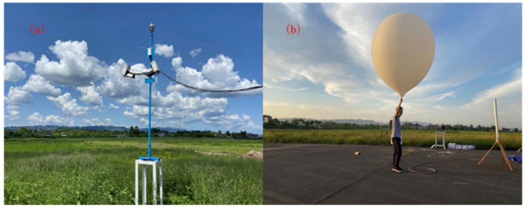
2. Experiments Details

Based on pulsed coherent Doppler lidar (PCDL), microwave radiometer, micro-thermometer, and radiosonde, a field campaign was conducted by the Anhui Institute of Optics and Fine Mechanics, Chinese Academy of Sciences, in 2021, to study the spatiotemporal evolutionary mechanism of optical turbulence in the northeast of the Sichuan Basin. The geographic location of the Sichuan Basin and the field campaign site is shown in Figure 1. The Sichuan Basin has a special geographical location, with the Qinghai–Tibet Plateau in the west and the middle and lower Yangtze plains in the east. In the northeast of the Sichuan Basin, there is a series of northeast–southwest valleys, and the test site was located in one of the wide valleys, where the altitude of the surrounding mountains was between 1500 and 2000 m. This altitude is within the range of the atmospheric boundary layer, which may have an important impact on the development of optical turbulence. With the unique topography and landforms, it will show different meteorological characteristics than other locations.

The PCDL is a scanning and remote sensing instrument that measures the wind field along the lidar beam. The PCDL used here was from the Southwest Institute of Technical Physics, and its technical parameters are shown in

Table 1. The main technical parameters of the PCDL.

Parameters	Wavelength (nm)	Detection Distance (m)	Wind Speed Detection Range (m/s)	Wind Direction Detection Range (°)	Vertical Resolution (m)
Value	1550	30–10,000	0–75	0–360	30/50/100/200

. The laser pulse width can be tuned to 500 ns, corresponding to a spatial resolution of 30 m in the radial direction and a temporal sampling rate of 4 Hz, with significant advantages in studying optical turbulent characteristics. The experimental site was in complex terrain surrounded by mountains. To gain the temperature field of the same site, a microwave radiometer was installed 10 m away. The microwave radiometer was produced and developed by the Sun Create Electronics Co., Ltd. Hefei, China, which provides temperature and pressure profiles with high spatial resolution (i.e., 50 m) and high temporal resolution (i.e., 1 s). The main technical parameters of the microwave radiometer are described in

Table 2. The main technical parameters of the microwave radiometer.

Parameters	Detection Distance (m)	Temperature Detection Range (°C)	Temporal Resolution (s)	Vertical Resolution (m)
Value	0–10,000	−60–40	1	50

. The above two pieces of equipment are shown in Figure 2. Using routine meteorological parameters, the temporal and spatial variation characteristics of optical turbulence strength could be estimated according to the existing $C_n^2$ model.

During the campaign, a micro-thermometer, from the Anhui Institute of Optics and Fine Mechanics, Chinese Academy of Sciences, was installed approximately 3 m over the Earth’s surface, and the daily variation in turbulence strength near the ground was obtained [20,21,22,23]. A comprehensive description of the micro-thermometer and its specifications are given in [4,24,25]. The installation location of the instrument and the surrounding environment are shown in Figure 3a. In order to improve the turbulence strength estimation model to make it more suitable for the site, a balloon-borne radiosonde equipped with micro-thermometers and GPS was launched at the experimental site as shown in Figure 3b. The working status and available meteorological parameters provided by each instrument are described in

Table 3. Working conditions of the instruments.

Instruments	Measurement Parameters	Working Status
PCDL	Wind speed, wind direction	Continuous
Microwave radiometer	Temperature, humidity	Continuous
Micro-thermometer	Turbulence strength (3 m above ground level)	Continuous
Radiosonde	Turbulence strength (0–30 km)	Intermittent

.

3. Methodology of Estimating Optical Turbulence

3.1. Estimation Models

Parameterization models of optical turbulence have been developed to convert standard radiosonde meteorological parameters into vertical profiles of $C_n^2$, the refractive index structure constant [26]. According to Kolmogorov’s theory, which was under the assumption of local homogeneity and stationarity of the refractive index fluctuations, the parameterization model uses the Tatarskii model for estimating $C_n^2$ profiles as shown below [1]:

$$C_n^2=a{L}_0{}^{4/3}{M}^2$$

(1)

where $a$ is a dimensionless constant that is mostly used at a value of 2.8 [17]; $L_0$ is the outer scale, which is the largest scale of inertial range turbulence. The potential refractive index gradient, $M$, is expressed as:

$$M=-\left(\frac{79\times {10}^{-6}P}{T}\right)\frac{\partial \ln \theta }{\partial h}$$

(2)

$$\theta =T{\left(\frac{1000}{P}\right)}^{0.286}$$

(3)

where $M$ is related to atmospheric temperature $\left(T\right)$, atmospheric pressure $\left(P\right)$, and potential temperature $\left(\theta \right)$; $h$ is the height above ground. In addition, Tatarskii introduced Equation (1), which can be rewritten as:

$$C_n^2=a{\left[K^2/{(\frac{\partial \overrightarrow{V}}{\partial h})}^2\right]}^{1/3}{M}^2$$

(4)

where $\overrightarrow{V}$ is the horizontal wind velocity vector, and $K$ is the turbulent diffusion coefficient. $K$ can be expressed as:

$$K={\epsilon }_{TKE}/{\left(\partial \overrightarrow{V}/\partial h\right)}^2$$

(5)

where ${\epsilon }_{TKE}$ is the turbulence energy dissipation rate.

From Equations (1)–(3), it can be noted that the vertical temperature gradient can be estimated from sounding data; therefore, choosing the appropriate $L_0$ is the key to estimation $C_n^2$. At present, the HMNSP99 model and Dewan model are the most widely used outer scale model [27,28,29]. With the basics of the Tatarskii equation, an outer scale model was proposed by Dewan considering the vertical shear of the horizontal wind speed, and two expressions for the troposphere and stratosphere were proposed [26]. Trinquetet’s research indicated that the model needs to be used with a vertical resolution of 300 m, and $S$ must not exceed 0.04 s⁻¹ [30]. The outer scale is given as follows:

$$L_0{}^{4/3}=\{\begin{array}{l}{0.1}^{4/3}\times {10}^{1.64+42\times S},\mathrm{Troposphere}\\ {0.1}^{4/3}\times {10}^{0.506+50\times S},\mathrm{Stratosphere}\end{array}$$

(6)

where $S$ is the vertical shear of the horizontal velocity.

$$S=\sqrt{{\left(\frac{\partial u}{\partial h}\right)}^2+{\left(\frac{\partial v}{\partial h}\right)}^2}$$

(7)

where $u$ and $v$ are two horizontal wind components.

Another outer scale model was proposed by Ruggiero and DeBenedictis, called the HMNSP99 model, in which the outer scale is the function of $S$ and temperature gradient ($\frac{dT}{dh}$) simultaneously [31]. Due to the fact that it contains more atmospheric parameters, the model might be more in line with the nature of the actual development of turbulence:

$$L_0{}^{4/3}=\{\begin{array}{l}{0.1}^{4/3}\times {10}^{0.362+16.728S-192.347\frac{dT}{dh}},\mathrm{Troposphere}\\ {0.1}^{4/3}\times {10}^{0.757+13.819S-57.784\frac{dT}{dh}},\mathrm{Stratosphere}\end{array}$$

(8)

3.2. Integrated Astroclimatic Parameters

In AO applications, the laser beam does not always propagate to heights of tens of kilometers as is the case in astronomical applications and boundary-layer research. Quite often, the beam propagates through the atmosphere within several kilometers above the ground, a height for which the turbulence profile is not well behaved due to the ground effects. It is necessary to obtain integrated astroclimatic parameters including the atmospheric coherence length, $r_0$, and seeing $\epsilon$ to design and evaluate the AO system. The integrated value of $C_n^2$ allows us to predict the atmospheric optical quality in terms of seeing $\epsilon$ as well as the coherence length,$r_0$, that depends on the local conditions at altitude h. The seeing $\epsilon$ is a crucial parameter that leads us to distinguish the most effective windows in the AO systems, which can be used to retrieve $r_0$ [32]. All the parameters are given as follows:

$$r_0={\left[0.423{\left(\frac{2\pi }{\lambda }\right)}^2{\displaystyle {\int }_0^{\infty }{C}_n^2\left(h\right)dh}\right]}^{-3/5}$$

(9)

$$\epsilon =5.25{\lambda }^{-1/5}{\left({\displaystyle {\int }_0^{\infty }{C}_n^2\left(h\right)dh}\right)}^{3/5}$$

(10)

4. Results and Discussion

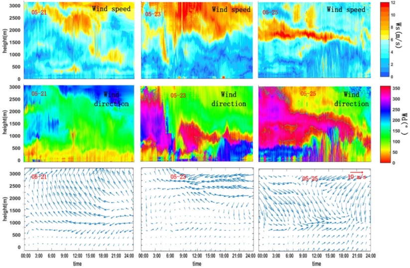
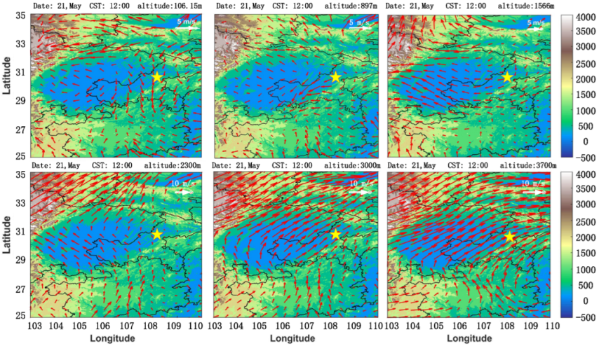
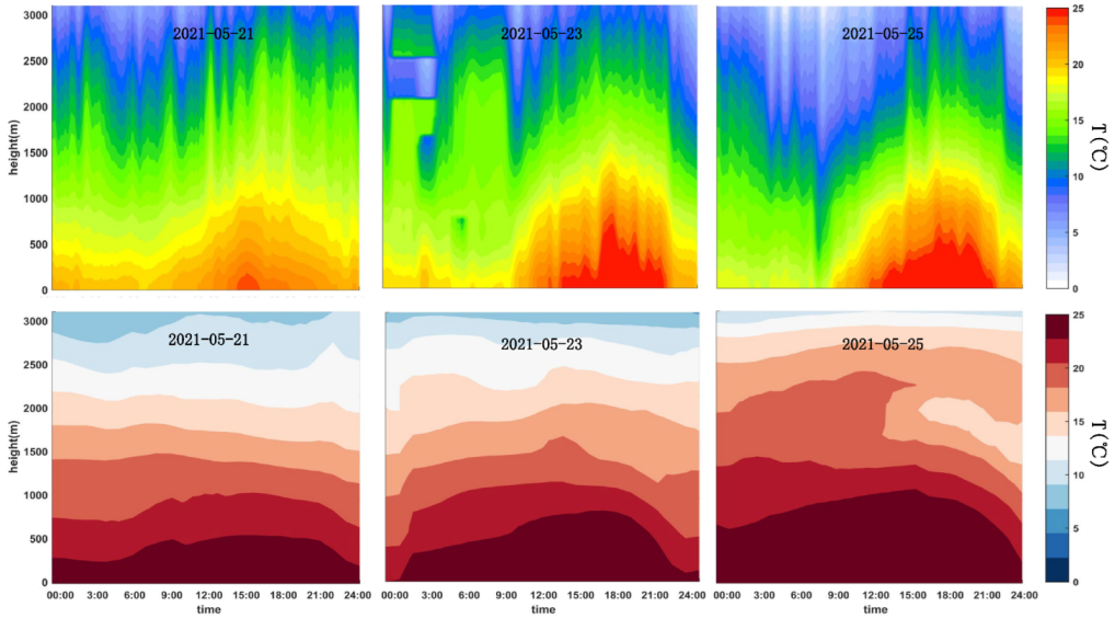
4.1. Characteristics of Basic Meteorological Parameters

Figure 4 shows the temporal and spatial characteristics of the wind speed and wind direction data from the PCDL at the experimental site and the ERA5 reanalysis data of the grid points near the experimental site. A comprehensive description of the ERA5 reanalysis data is given in [33]. Comparing the wind speed and direction data from the PCDL and ERA5, the results show that their diurnal variation with height distribution had good consistency. From the side, it is reasonable to use wind speed and wind direction data from the PCDL. As shown in Figure 4 (top), this may be due to the influence of the topography of the basin, where wind speed is relatively stable (i.e., below 1.5 km), and wind speed values were between 0 and 6 m/s. In contrast, high wind speeds began to appear above 1.5 km, with the maximum wind speed reaching 12 m/s. In addition, compared to the wind direction below 1.5 km, the wind direction above 1.5 km was relatively stable, where there was a wide range of relative fixed wind directions, since it was under the influence of the westerly zone as shown in Figure 4 (middle). The differences in wind direction may be attributed to the surrounding mountains that have a mutual effect on atmospheric conditions. Due to the influence of the special terrain, it can be predicted that there is a large wind shear near the peaks around the basin. It should be noted that there is a difference between the location of the grid point area obtained by satellite data and the site where the measuring equipment was located; thus, the two data were not exactly the same, but their trend was very close.

To better explain the vertical distribution of wind speed and direction, Figure 5 shows the corresponding changes at 12:00 on 21 May at different AGL heights (106.15, 897, 1566, 2300, 3000, and 3700 m). The white arrows represent the magnitude and direction of the wind speed and the yellow five-pointed stars the campaign site. In the Sichuan Basin, the wind speed at heights of 106.15 and 897 m was slow, and there was no uniform wind direction. At a height of 1566 m, the wind speed over the basin is still very small, but the wind direction tended to be consistent. In contrast, the wind speed increased, and the wind direction was consistent as the height increased. After the height reached to 3700 m, the wind direction over the entire basin was consistent with the outside of the basin. The spatial difference in wind speed and wind direction could be the result of the terrain, which had good agreement with the results obtained by PCDL. The Sichuan Basin can be regarded as a semi-enclosed space. Inside the space, the wind speed and direction of each location developed independently, so the wind speed was different and showed different wind directions. Outside the space, due to the influence of the westerly zone, the wind speed increased overall, and the wind direction tended to be consistent.

Similarly, the spatiotemporal distribution of the temperature from the microwave radiometer and ERA5 reanalysis data are shown in Figure 6. The temperature had an obvious diurnal variation trend, which reached its maximum between 15:00 and 16:00. Weather had an obvious effect on the vertical distribution of temperature; for example, on 25 May, after a drizzle, there was a heavy rain between 7:00 and 9:00, and then the sun was shining. Compared with the pictures obtained from the microwave radiometer, the ERA5 data did not accurately reflect the real-time changes in the temperature due to the fact of its lower resolution, but they still displayed the same temperature change trends.

4.2. Modification of HMNSP99 Outer Scale Model

To better investigate the optical turbulence spatiotemporal characteristics, two outer scale models are chosen here to estimate $C_n^2$ profiles, including Dewan model and HMNSP99 model as mentioned above. The comparison of $C_n^2$ profiles between measurements and calculation from models is depicted in Figure 7. The red line is the measured optical turbulence strength obtained by the micro-thermometer carried by meteorological balloon, others are derived by the PCDL and microwave radiometer based on models. It is obvious that the Dewan model is likely to overestimate the turbulence strength especially at high altitudes. Compared to Dewan model, the estimated profile values using the HMNSP99 model are more consistent with the measured values. However, the error between the calculated value and the measured value is still large.

In order to better reconstruct the optical turbulence strength of the experimental site, a new statistical outer scale model was improved based on the HMNSP99 model using the meteorological balloons’ data. The statistical average of the vertical profiles of $L_0$, $S$, and $\frac{dT}{dh}$ were acquired with a vertical resolution of 30 m, and the exponent of the formula was refitted by the least squares method. The modified HMNSP99 model was characterized as Equation (11). The $C_n^2$ profiles estimated by the modified HMNSP99 model are also illustrated in Figure 7. Although it is difficult to describe the optical turbulence’s fine structure precisely, the model can reflect the trend in the optical turbulence’s variation to some extent.

$$L_0{}^{4/3}={0.1}^{4/3}\times {10}^{1.242+8.663S-86.732\frac{dT}{dh}}$$

(11)

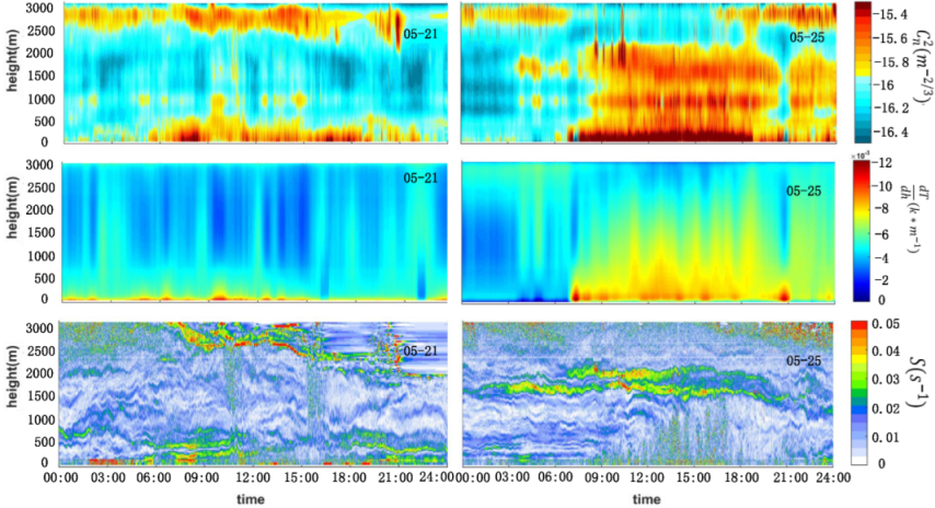
4.3. Spatiotemporal Characteristics and Effect Factors of Optical Turbulence

Using basic meteorological parameters from the PCDL and microwave radiometer, the spatiotemporal variation of $C_n^2$ estimated by the modified HMNSP99 model is illustrated in Figure 8. Both 21 and 25 May were selected to display the spatiotemporal variation in the optical turbulence and corresponding affecting factors. It is noted that in the two figures, the values of $\log C_n^2$ were basically above −16.5 m^–2/3, and the values seem to be consistent with Masciadri’s studies [34]. In order to investigate the factors affecting the development process of turbulence, Figure 8 also shows the temporal and spatial diurnal variation characteristics of temperature gradient ($\frac{dT}{dh}$) and wind shear ($S$). It is obvious that the optical turbulence strength and temperature gradient were in good agreement under 2 km, that is, the greater the temperature gradient, the stronger the turbulence strength. Moreover, the strong turbulent layer above 2 km, especially from 2.5 to 3 km, was related more to wind shear, where there was an increase in the influence of wind shear and a decrease in the influence of temperature gradient.

Overall, in the process of optical turbulence development, temperature gradient plays a dominant role in turbulence generation below 2 km, and wind shear plays an important role above 2 km. Optical turbulence is also affected by the basin terrain. Due to the low altitude of the field campaign site, it was almost surrounded by mountains, which isolated the turbulence inside it; thus, optical turbulence developed independently and was mainly affected by the temperature gradient. Over the basin, the strong wind in the westerly zone and the weak wind at the top of the basin formed a large wind shear, the influence of which far exceeded the temperature gradient and played a leading role in the development of optical turbulence.

Based on the PCDL and microwave radiometer data, the diurnal variation curves of the turbulence strength at different altitudes were obtained, and they are depicted in Figure 9. As can be seen, for turbulence mainly deduced by temperature gradient, its strength gradually decreases with the increase in altitude. The refractive index structure constant had a relatively typical “Sombrero” feature at different altitudes, which gradually disappear with the increase in altitude. Notably, there was a little more disagreement between the two days’ diurnal variation curves of turbulence strength, where the typical “Sombrero” feature disappeared at 704 and 2055 m, respectively. The reason for this was that on 21 May it was cloudy, while on 25 May it was mainly sunny. The development of optical turbulence in the boundary layer is closely related to air temperature. Similarly, the diurnal variation curves of the surface layer, $C_n^2$, from the micro-thermometer are clearly illustrated in Figure 9c. Compared with the turbulence strength on 21 May, the strength on 25 May was significantly enhanced, and strong turbulence existed for a longer time. From Figure 6, the air temperature on 21 May was lower than that on 25 May. Only the air temperature near the ground reached 25 °C at 15:00 on 21 May. Compared with 21 May, the high temperature lasted longer on 25 May, and the maximum height reached 0.5 km. Differences in the air temperature resulted in the strength of the optical turbulence and limited the maximum height of turbulence development.

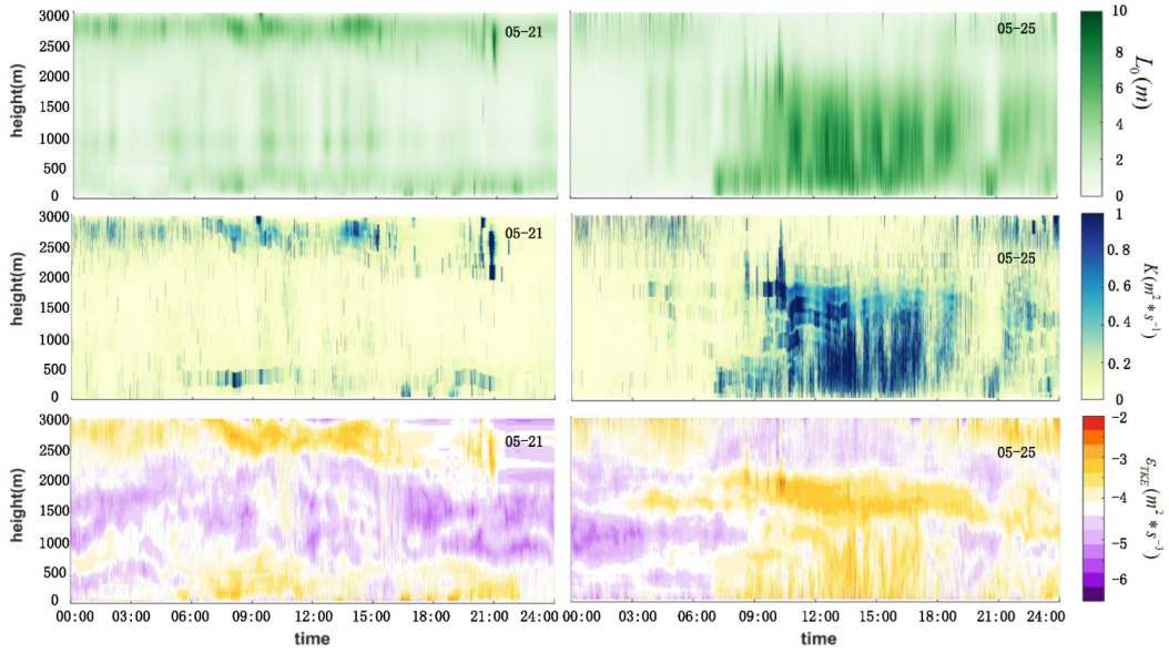
4.4. Spatiotemporal Characteristics of Turbulence Basic Parameters

According to Equations (1) and (4), we can calculate the optical turbulence strength if given the outer scale $L_0$, turbulence diffusion coefficient $K$, turbulence energy dissipation rate ${\epsilon }_{TKE}$, and the corresponding conventional meteorological parameters. It is necessary to obtain the spatiotemporal characteristics of basic turbulence parameters. Figure 10 presents the results derived from conventional meteorological parameters of the experimental site. It is apparent that $L_0$ agrees well with $C_n^2$ in the temporal and spatial characteristics, where turbulence strength increases as the outer scale increases. The relationship between $C_n^2$ and $L_0$ accords with our earlier observations that showed that $L_0$ has the biggest influence weight among the turbulence influence factors [22]. In addition, the value of $L_0$ agrees with Takato’s (1995) findings that found that $L_0$ is basically in the range of 1–10 m [35]. $K$, ${\epsilon }_{TKE}$, and $C_n^2$ in this study also had good consistency, where $K$ and ${\epsilon }_{TKE}$ could reflect the strength of the turbulence from the side. The results, as shown in the middle and bottom of Figure 10, indicate that the values of $K$ and ${\epsilon }_{TKE}$ were basically in the range of 0–1 m²·s⁻¹ and 10⁻⁶–10⁻³ m²·s⁻³, respectively. There was a significant positive correlation between these basic turbulence parameters. Moreover, no report was seen that a complete spatiotemporal distribution of $L_0$, $K$, and ${\epsilon }_{TKE}$ was obtained from the PCDL at the same time.

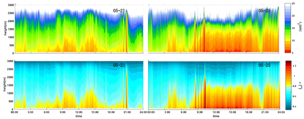
4.5. Spatiotemporal Characteristics of Astronomical Parameters

Figure 11 provides the temporal and spatial characteristics of integrated astronomical parameters (the atmospheric coherence length $r_0$, seeing $\epsilon$) at the experimental site. It was apparent that $r_0$ had relative typical diurnal variation characteristics and, on the whole, increased with height at different times. The coherence length was smaller between approximately 07:00 and 20:00 and larger at other times. Comparing the results of the two days, $r_0$ on 21 May was larger than that on 25 May after 7:00 in the daytime. As Figure 11 shows, there was an opposite diurnal characteristic between $r_0$ and $\epsilon$. The whole trend of $\epsilon$ decreased with height at different times, which had good agreement with Mchugh’s investments [36]. Moreover, $\epsilon$ was larger between approximately 07:00 and 20:00, and smaller at other times. The $\epsilon$ from May 25 can be compared with $\epsilon$ on the May 21, which shows that there was a strong seeing layer below 2 km during the daytime. It is difficult to explain this result, but the different diurnal characteristics might be related to the season and weather conditions.

According to Equations (9) and (10), the diurnal variation curves of the integrated atmospheric parameters of the two days are presented in Figure 12. The $r_0$ and $\epsilon$ on 25 May had typical diurnal characteristics. The general trend for $r_0$ was that it was smaller during the daytime and larger at nighttime, reaching a minimum value of 5 cm. On the contrary, $\epsilon$ was larger during the daytime and smaller at night. A positive correlation is found between $\epsilon$ and $C_n^2$, and the result seems to be consistent with Tian’s research that suggested that such a seeing minimum had a good temporal association with the $C_n^2$ minimum simultaneously observed at ATS [37]. Compared with the results obtained on 25 May, the diurnal variation of $r_0$ and $\epsilon$ on 21 May was weakened. There was not much difference between $r_0$ and $\epsilon$ for the two days at before approximately 07:00 and after approximately 20:00. A possible explanation for these differences may be that 21 May can be regarded as close to stable atmospheric conditions, since it was overcast, and on 25 May it was sunny. The above results provide further knowledge for the space–time characteristics of the astronomical parameters of the basin.

5. Conclusions

Since the late 1960s, many research communities have shown an interest in measuring and estimating optical turbulence profiles. Most of the profiles are measured at different time periods or at a single measuring point, for example, using a radiosonde or an ultrasonic anemometer, which cannot reflect the spatiotemporal variation of optical turbulence. Appropriate knowledge of the spatiotemporal characteristics of $C_n^2$ is important, since laser transmission and astronomical observation are severely affected by optical turbulence. In this investigation, the spatiotemporal variation of $C_n^2$ was estimated using basic meteorological parameters derived from PCDL and a microwave radiometer. Moreover, the integrated parameters for astronomy and optical telecommunication were derived from optical turbulence strength profiles at the experimental site. The corresponding conclusions are as follows.

(1) Due to the fact that temperature gradient and wind shear play important roles in the development of turbulence, they are applied to various parameterized models. However, the proportion of temperature gradient and wind shear in the model will be affected by time, altitude, environment, and other factors. In this paper, in order to obtain the temporal and spatial variation characteristics of turbulence strength over the basin, on the basis of the original HMNSP99 model, a new parametric model was obtained through fitting the $C_n^2$ profile measured by balloon-borne micro-thermometer. Compared with the original HMNSP99 model, the modified model had better environmental adaptability;

(2) Usually, $C_n^2$ has a large value near the ground and decreases with height. Turbulence strength was stronger during the daytime and weaker at nighttime. The temperature gradient and wind shear together affected the development of optical turbulence. However, due to the existence of the basin, the development of optical turbulence was affected. The basin can be regarded as a semi-enclosed space, where meteorological parameters in the basin develop independently and avoid outside factors, while external affecting will increase above the basin. The lower wind speed in the basin directly weakened the influence of wind shear, which increased the effect of temperature gradient. There was a strong turbulence layer above the basin, especially between 2.5 and 3 km, which may mainly be caused by the combined action of the westerly zone and topography. Moreover, the differences in the optical turbulence strength between the two days in Figure 8 were relatively large, from 0.5 to 2 km, which may be related to the generation and elimination mechanism of turbulence;

(3) Under the main influence of the temperature gradient inside the basin, the $C_n^2$ had a relatively typical “Sombrero” feature at different altitudes, which gradually disappeared with the increase in altitude. Over the basin, although there was also a strong turbulence layer under the main influence of wind shear, the diurnal variation in turbulence also did not appear. Under the influence of temperature gradient and wind shear, optical turbulence exhibited different temporal and spatial characteristics. The results of this study indicate that in the process of optical turbulence development, temperature gradient plays a dominant role in turbulence generation below 2 km and wind shear has an important influence above 2 km.

(4) This is the first time that several complete 3D maps of optical turbulence parameters, from the ground up to 3 km, were obtained from PCDL at the same time. Unlike other previous attempts, our results cover a wide variety of time, space, and parameters. The consistency of variations in multiple parameters increases the reliability of the results. From the results, we can conclude that in the basin environment, the approximate ranges of the outer scale, turbulence diffusion coefficient, and turbulent energy dissipation rate were 1–10 m, 0–1 m²·s⁻¹, and 10⁻⁶–10⁻³ m²·s⁻³, respectively. Moreover, the spatiotemporal characteristics of the astronomical parameters derived from the optical turbulence profiles are present in this work. The integrated astronomical parameters had typical diurnal characteristics, where the general trend for $r_0$ was that it was smaller during the daytime and larger at night, while $\epsilon$ was larger during the daytime and smaller at night. This leads to a better understanding of the behavior of these parameters relevant to the optical quality of the atmosphere from the ground up to 3 km.

These findings enhance our understanding of the spatiotemporal characteristics of $C_n^2$ under the influence of complex terrain. However, the findings in this investigation are subject to at least two limitations. First, the current study was limited by the size of experimental data set. A number of possible future studies using the same experimental setup are apparent, which will increase the persuasiveness of the experimental conclusions. Second, due to the limitations of the experimental equipment’s parameters, the current research did not specifically indicate the relationship of wind shear related to optical turbulence strength over the basin. It is suggested that the association of these factors be investigated in future studies. Notwithstanding these limitations, the findings are of significance for laser transmission and astronomical observation.

References

1. Tatarski, V.I.; Silverman, R.A.; Chako, N. Wave Propagation in a Turbulent Medium. Phys. Today 1961, 14, 46. [Google Scholar] [CrossRef]
2. Hutt, D.L. Modeling and measurement of atmospheric optical turbulence over land. Opt. Eng. 1999, 38, 1288–1295. [Google Scholar] [CrossRef]
3. Roddier, F. V The Effects of Atmospheric Turbulence in Optical Astronomy. In Progress in Optics; Wolf, E., Ed.; Elsevier: Amsterdam, The Netherlands, 1981; Volume 19, pp. 281–376. [Google Scholar]
4. Fried, D.L.; Mevers, G.E.; Keister, M.P. Measurements of Laser-Beam Scintillation in the Atmosphere. J. Opt. Soc. Am. 1967, 57, 787–797. [Google Scholar] [CrossRef]
5. Scipión, D.E.; Lawrence, D.A.; Milla, M.A.; Woodman, R.F.; Lume, D.A.; Balsley, B.B. Simultaneous observations of structure function parameter of refractive index using a high-resolution radar and the DataHawk small airborne measurement system. Ann. Geophys. 2016, 34, 767–780. [Google Scholar] [CrossRef] [Green Version]
6. Shao, S.; Qin, F.; Liu, Q.; Xu, M.; Cheng, X. Turbulent Structure Function Analysis Using Wireless Micro-Thermometer. IEEE Access 2020, 8, 123929–123937. [Google Scholar] [CrossRef]
7. Xiaoqing, W.U.; Qiguo, T.; Peng, J.; Bo, C.; Qing, C.; Jun, C.A.I.; Xinmiao, J.I.N.; Hongyan, Z. A new method of measuring optical turbulence of atmospheric surface layer at Antarctic Taishan Station with ultrasonic anemometer. Adv. Polar Sci. 2015, 26, 305. [Google Scholar] [CrossRef]
8. Vernin, J.; Barletti, R.; Ceppatelli, G.; Paternò, L.; Righini, A.; Speroni, N. Optical remote sensing of atmospheric turbulence: A comparison with simultaneous thermal measurements. Appl. Opt. 1979, 18, 243–247. [Google Scholar] [CrossRef] [PubMed]
9. Anand, N.; Sunilkumar, K.; Satheesh, S.K.; Moorthy, K.K. Entanglement of near-surface optical turbulence to atmospheric boundary layer dynamics and particulate concentration: Implications for optical wireless communication systems. Appl. Opt. 2020, 59, 1471–1483. [Google Scholar] [CrossRef] [PubMed]
10. Miller, M.; Zieske, P. Turbulence Environment Characterization; Interim Report; Avco-Everett Research Lab.: Everett, MA, USA, 1979; p. 135. [Google Scholar]
11. Good, R.E.; Beland, R.R.; Murphy, E.A.; Brown, J.H.; Dewan, E.M. Atmospheric models of optical turbulence. Proc. SPIE 1988, 928, 165–186. [Google Scholar] [CrossRef]
12. Jumper, G.; Beland, R. Progress in the understanding and modeling of atmospheric optical turbulence. In Proceedings of the 31st Plasmadynamics and Lasers Conference, Denver, CO, USA, 19–22 June 2000. [Google Scholar]
13. Beland, R.R.; Brown, J.H. A deterministic temperature model for stratospheric optical turbulence. Phys. Scr. 1988, 37, 419–423. [Google Scholar] [CrossRef]
14. Nath, D.; Venkat Ratnam, M.; Patra, A.K.; Krishna Murthy, B.V.; Bhaskar Rao, S.V. Turbulence characteristics over tropical station Gadanki (13.5°N, 79.2°E) estimated using high-resolution GPS radiosonde data. J. Geophys. Res. Atmos. 2010, 115, D07102. [Google Scholar] [CrossRef]
15. Hufnagel, R.; Stanley, N. Modulation Transfer Function Associated with Image Transmission through Turbulent Media. JOSA 1964, 54, 52–60. [Google Scholar] [CrossRef]
16. Warnock, J.M.; Vanzandt, T.E. A statistical model to estimate refractivity turbulence structure constant Cn2 in the free atmosphere. Int. Counc. Sci. Unions Middle Atmos. Program. Handb. MAP 1986, 20, 166. [Google Scholar]
17. Abahamid, A.; Jabiri, A.; Vernin, J.; Zouhair, B.; Azouit, M.; Agabi, A. Optical turbulence modeling in the boundary layer and free atmosphere using instrumented meteorological balloons. Astron. Astrophys. 2004, 416, 1193–1200. [Google Scholar] [CrossRef] [Green Version]
18. Bi, C.; Qian, X.; Liu, Q.; Zhu, W.; Li, X.; Luo, T.; Wu, X.; Qing, C. Estimating and measurement of atmospheric optical turbulence accordingto balloon-borne radiosonde for three sites in China. J. Opt. Soc. Am. A 2020, 37, 1785–1794. [Google Scholar] [CrossRef]
19. Zhang, R.; Jing, J.; Tao, J.; Hsu, S.C.; Wang, G.; Cao, J.; Lee, C.S.L.; Zhu, L.; Chen, Z.; Zhao, Y.; et al. Chemical characterization and source apportionment of PM2.5 in Beijing: Seasonal perspective. Atmos. Chem. Phys. 2013, 13, 7053–7074. [Google Scholar] [CrossRef] [Green Version]
20. Qing, C.; Wu, X.; Li, X.; Zhu, W. Performance analysis of weather research and forecasting model for simulating near-surface optical turbulence over land. Optik 2019, 188, 225–232. [Google Scholar] [CrossRef]
21. Qing, C.; Wu, X.; Li, X.; Zhu, W.; Qiao, C.; Rao, R.; Mei, H. Use of weather research and forecasting model outputs to obtain near-surface refractive index structure constant over the ocean. Opt. Express 2016, 24, 13303–13315. [Google Scholar] [CrossRef]
22. Shao, S.; Qin, F.; Xu, M.; Liu, Q.; Han, Y.; Xu, Z. Temporal and spatial variation of refractive index structure coefficient over South China sea. Results Eng. 2020, 9, 100191. [Google Scholar] [CrossRef]
23. Su, C.; Wu, X.; Luo, T.; Wu, S.; Qing, C. Adaptive niche-genetic algorithm based on backpropagation neural network for atmospheric turbulence forecasting. Appl. Opt. 2020, 59, 3699–3705. [Google Scholar] [CrossRef]
24. Beland, R.R. Propagation through atmospheric optical turbulence. In The Infrared and Electro-Optical Systems Handbook; Infrared Information Analysis Center: Ann Arbor, MI, USA, 1993; pp. 157–232. [Google Scholar]
25. Bufton, J. Correlation of Microthermal Turbulence Data with Meteorological Soundings in the Troposphere. J. Atmos. Sci. 1973, 30, 83–87. [Google Scholar] [CrossRef]
26. Dewan, E.; Good, R.; Beland, R.; Brown, J. A Model for Cn(2) (Optical Turbulence) Profiles Using Radiosonde Data; Directorate of Geophysics, Air Force Materiel Command: MA, USA, 1993; p. 50. Available online: https://www.semanticscholar.org/paper/A-Model-for-Csubn(2)-(Optical-Turbulence)-Profiles-Dewan-Good/b202d31abb56ab8af7810f1c26d9135e436d46b8 (accessed on 16 February 2022).
27. Han, Y.; Wu, X.; Luo, T.; Qing, C.; Yang, Q.; Jin, X.; Liu, N.; Wu, S.; Su, C. New Cn2 statistical model based on first radiosonde turbulence observation over Lhasa. J. Opt. Soc. Am. A 2020, 37, 995–1001. [Google Scholar] [CrossRef]
28. Cai, J.; Li, X.B.; Zhan, G.W.; Wu, P.F.; Xu, C.Y.; Qing, C.; Wu, X.Q. A new model for the profiles of optical turbulence outer scale and Cn2 on the coast. Wuli Xuebao/Acta Phys. Sin. 2018, 67, 137–151. [Google Scholar] [CrossRef]
29. Qing, C.; Wu, X.; Li, X.; Luo, T.; Su, C.; Zhu, W. Mesoscale optical turbulence simulations above Tibetan Plateau: First attempt. Opt. Express 2020, 28, 4571–4586. [Google Scholar] [CrossRef]
30. Trinquet, H.; Vernin, J. A Model to Forecast Seeing and Estimate C2N Profiles from Meteorological Data. Publ. Astron. Soc. Pac. 2006, 118, 756–764. [Google Scholar] [CrossRef] [Green Version]
31. Ruggiero, F.H.; Debenedictis, F.H. Forecasting optical turbulence from mesoscale numerical weather prediction models. In Proceedings of the DoD High Performance Modernization Program Users Group Conference, Austin, TX, USA, 10–14 June 2002. [Google Scholar]
32. Roddier, F.; Gilli, J.M.; Lund, G. On the origin of speckle boiling and its effects in stellar speckle interferometry. J. Opt. 2000, 13, 263. [Google Scholar] [CrossRef]
33. Han, Y.; Yang, Q.; Nana, L.; Zhang, K.; Qing, C.; Li, X.; Wu, X.; Luo, T. Analysis of wind-speed profiles and optical turbulence above Gaomeigu and the Tibetan Plateau using ERA5 data. Mon. Not. R. Astron. Soc. 2021, 501, 4692–4702. [Google Scholar] [CrossRef]
34. Masciadri, E.; Vernin, J.; Bougeault, P.J.A. 3D numerical simulations of optical turbulence at the Roque de Los Muchachos Observatory using the atmospherical model Meso-Nh. Astron. Astrophys. 2001, 365, 699–708. [Google Scholar] [CrossRef] [Green Version]
35. Takato, N.; Yamaguchi, I. Spatial correlation of Zernike phase-expansion coefficients for atmospheric turbulence with finite outer scale. J. Opt. Soc. Am. A 1995, 12, 958–963. [Google Scholar] [CrossRef]
36. McHugh, J.; Jumper, G.; Chun, M. Balloon Thermosonde Measurements over Mauna Kea and Comparison with Seeing Measurements. Publ. Astron. Soc. Pac. 2008, 120, 1318–1324. [Google Scholar] [CrossRef]
37. Tian, Q.; Jiang, P.; Jin, X.; Li, J.; Pei, C.; Du, F.; Li, Z.; Li, X.; Chen, H.; Ji, T.; et al. Discovery of high-quality daytime seeing windows at the Antarctic Taishan station. Mon. Not. R. Astron. Soc. 2020, 493, 5648–5652. [Google Scholar] [CrossRef]
Figure 1. Geographic location of the Sichuan Basin and the field campaign site represented by the five-pointed star.
Photonics 09 00235 g001
Figure 2. Experimental scenario of (a) the pulsed coherent Doppler lidar and (b) the microwave radiometer.
Photonics 09 00235 g002
Figure 3. Photographs of (a) the micro-thermometer and (b) the balloon-borne micro-thermometer.
Photonics 09 00235 g003
Figure 4. Spatiotemporal distribution of wind speed and wind direction from the PCDL (top and middle) and the ERA5 reanalysis data (bottom).
Photonics 09 00235 g004
Figure 5. Wind speed and direction from the ERA5 reanalysis at different heights; the yellow five-pointed star represents the campaign site.
Photonics 09 00235 g005
Figure 6. Spatiotemporal distribution of temperature from microwave radiometer (top) and ERA5 reanalysis data (bottom).
Photonics 09 00235 g006
Figure 7. Comparison of the C n 2 profiles between measurements conducted by the meteorological balloons and calculations by different outer scale models including HMNSP99, the modified HMNSP99, and Dewan.
Photonics 09 00235 g007
Figure 8. Spatiotemporal distribution of C n 2 , d T d h , and S in two days.
Photonics 09 00235 g008
Figure 9. Diurnal profiles of C n 2 at different altitudes, (a) May 21; (b) May 25; (c) surface.
Photonics 09 00235 g009
Figure 10. Spatiotemporal distribution of L 0 , K , and ε T K E in two days.
Photonics 09 00235 g010
Figure 11. Spatiotemporal distribution of r 0 and ε during the two days.
Photonics 09 00235 g011
Figure 12. Diurnal profiles of r 0 and ε over the two days.
Photonics 09 00235 g012