Mitigating Vortex Splitting by Controlling the Wavefront Isophase Line Curvature of Vector Autofocusing Airy Vortex Beams in Free Space

Abstract

The match between the orbital angular momentum (OAM) transmission and receipt is a prerequisite for vortex beams as a carrier of the wireless optical communication system in free space. However, the vortex splitting induced by atmospheric turbulence results in an offset in the average OAM measured after propagating over the free space optical communication link. Therefore, how to reduce the vortex splitting effect to improve the stability of orbital angular momentum propagation is studied in this paper. First, a new parameter $(m)$ is introduced to modulate the radial distribution of the polarization state of the autofocusing Airy vortex beams (AAVBs). Second, to control the optical field distribution in focal plane, the wavefront isophase line curvature of the AAVBs is reconstructed by using the Pancharatnam-Berry phase generated in the polarization conversion process. Finally, by comparing the vortex splitting rates of the AAVBs with different wavefrontisophase line curvatures under different turbulence environments, it can be found that the vortex splitting in free space can be effectively mitigated by choosing an appropriate wavefront isophase line curvature. In addition, the mitigation effect is more obvious in the atmosphere with stronger turbulence. This study provides a new feasible method to control the phase structure of vortex beams and promises potential applications in the OAM-based free space optical communication system.

1. Introduction

A phase singularity nested in the cross section of the coherent beam can form a vortex beam with a spiral wavefront [1], and its Poynting vector propagates along the spiral [2]. The typical feature of vortex beams is that the phase factor $\exp (il\phi )$ is ubiquitous in the phase structure. On average, each photon in a vortex beam carries the orbital angular momentum (OAM) of $\pm l\hslash$ [3], where $l$ is the quantum number (also known as topological charge), which is generally an integer or a fraction [4]. The rapid development of OAMbased coding and multiplexing technology in recent years has made OAM a new degree of freedom for encoding information [5,6].

Due to the application value of the vortex beam as an information carrier in improving communication capacity and spectral efficiency [7], it has become a research hotspot in the field of free space optical communication. However, influenced by turbulent effects including beam wander [8], scintillation [9], OAM modes crosstalk [10], and so on, and due to the divergence of the optical vortex beams themselves [11], the transmitted information will randomly fluctuate at the communication system receiver. In order to mitigate the divergence of vortex beams, a series of structured beams with non-diffracting and self-healing properties in recent years have been widely used as the background to nest vortices [12,13,14]. Among them, autofocusing Airy beams managed to catch attention due to their unique focusing characteristics, which can effectively weaken the beam spread effect caused by atmospheric turbulence [15]. In recent years, the propagation characteristics of autofocusing Airy vortex beams (AAVBs) in free space have been extensively studied [16,17,18]. Since not being satisfied with the turbulence-resistant capability inherent in AAVBs, researchers have further regulated the phase structures to obtain better transmission features. For example, AAVBs with nontraditional spiral phases, represented by the power exponential spiral phase [19,20,21], have been successively proposed [22,23,24]. Although the focusing ability of these new vortex beams is significantly enhanced compared with that of the traditional AAVBs, the vortex splitting phenomenon occurs obviously even when the beams transmit in homogeneous medium. According to the research, vortex splitting will lead to the OAM transmit–receive mismatch [25] in the communication system, resulting in serious distortions of the information transmitted. Therefore, the aim of this paper is to study the way to effectively reduce the vortex splitting in free space when strengthening the focusing ability of AAVBs. In addition, the advantages of the polarization state as the degree of freedom of the light field are not considered in the above literature. More and more studies have shown that the non-uniform modulation of the polarization states of vortex beams can control the energy distribution and spin-orbit angular momentum coupling of light fields in free space propagation [26].

Through further study of the above nontraditional spiral phase regulation mechanism, we found that the reason for the deepening of the vortex splitting phenomenon is that the rotational symmetry of the traditional spiral phase is broken. In this paper, the phase of the AAVBs with radial-variant polarization is modulated by the Pancharatnam- Berry phase that is closely related to the variation of polarization state, and a new form of nontraditional spiral phase is proposed. The characteristic of this nontraditional spiral phase is that the wavefront isophase line is curved (here, the tailored wavefront isophase line is curved in source plane, not straight in tradition) while maintaining the rotational symmetry of the traditional spiral phase. Based on the generalized Huygens Fresnel principle and multilayer random phase screen theory, a model of radially polarized AAVBs propagation in atmospheric turbulence is established. On this basis, it is proven that the AAVBs with radial polarization variation are more advantageous than the traditional scalar AAVBs in restraining vortex splitting caused by atmospheric turbulence.

2. Methods

The electric field intensity of the AAVBs with radial-variant polarization in the source plane [27] can be rewritten as

$$E(r,\phi ) = Ai\left(\frac{r_0 - r}{\omega }\right)\exp \left(a \cdot \frac{r_0 - r}{\omega }\right)\exp (il\phi )\left[\sin \left(\frac{2n\pi r^m}{R} + {\phi }_0\right){\widehat{e}}_x + i\cos \left(\frac{2n\pi r^m}{R} + {\phi }_0\right){\widehat{e}}_y\right]$$

(1)

where $l$ is the topological charge, $(r,\phi )$ is the polar coordinate, $Ai(\cdot )$ represents Airy function, $r_0$ is the radius of the main ring, $\omega$ is the cross-section scale factor, $a$ is the apodization factor, $n$ and $m$ are the radial polarization indices, and ${\phi }_0$ is the parameter regulating the overall polarization states of the light field. It should be noted that Equation (1) in this paper differs from that in the literature [27] in the following three points: first, the spiral phase factor $\exp (il\phi )$ and the radial polarization regulation index $m$ are added in this paper; second, $R$ is the radius of the light field, not the radius of the main ring in the literature [27]; third, ${\phi }_0$ in Equation (1) in this paper is a parameter describing the overall polarization state of the light field, while ${\phi }_0$ in the literature [27] represents the polarization state at $r = 0$.

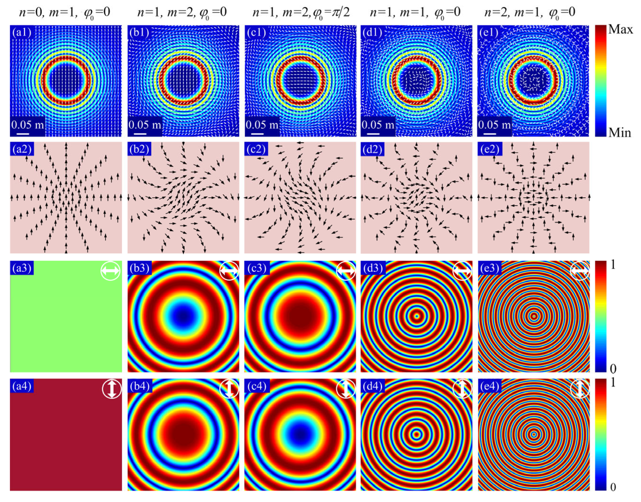
By solving Equation (1), the influence of $m$, $n$, and ${\phi }_0$ on the radial distribution of the polarization states of the autofocusing Airy beams can be obtained, as shown in Figure 1. The parameters used for calculation were set as: $l = 0$, wavelength $\lambda = 1550 \mathrm{nm}$, main ring radius $r_0 = 0.093 \mathrm{m}$, cross-section scale factor $w = 0.012$, apodization factor $a = 0.1$, and light field radius $R = 0.256 \mathrm{m}$. In Figure 1, the first row is the polarization state distribu- tions of the light field under different radial polarization indices. The second row is a sim- plified schematic to clearly describe the regularity of polarization state change shown in the first row. The third and fourth rows are the horizontal and vertical components of the polarization distribution shown in the first row, respectively. Figure 1(a1–a4) shows the polarization distribution of the scalar autofocusing Airy beams, and Figure 1(b1–b4, c1–c4, d1–d4, e1–e4) shows the polarization distributions of the vector autofocusing Airy beams. As shown in Figure 1(b1,b2), the polarization states of the light field rotate clockwise along the radius direction from the center of the light field. By comparing Figure 1(b2) with Figure 1(c2), it can be found that the polarization states of the light field rotate as a whole with the change of ${\phi }_0$. By comparing Figure 1(d2) with Figure 1(e2), it can be found that, with the increase of $n$, the radial change frequency of the beam polarization state is obviously accelerated. The reasons are as follows: as can be seen from the expression $\phi = 2n\pi r^m/R + {\phi }_0$, when $n = 1$, $m = 1$, $\phi$ increases by $2\pi$ (one period) in the process of $r$ increasing from 0 to $R$. As shown in Figure 1(d2), the light field is vertically polarized at $r = 0$ and deflected with the increase of $r$. However, when $r$ increases to $R$, the polarization state of the light field returns to the vertical polarization state, that is, a period of change is completed. With the further increase of $n$, a period of change is completed as $r$ increases from 0 to $R/n(n > 1)$. Therefore, the radial polarization state change frequency of the light field increases with the increase of the radial polarization index $n$, as shown in Figure 1(d3,e3,d4,e4). By comparing Figure 1(d1–d4) with Figure 1(b1–b4), it can be found that with the increase of $m$, the radial change frequency of the beam polarization state becomes smaller, because $r \le R < 1$ in this paper, when $m > 1$, $r^m < R$, $\phi$ cannot change by $2\pi$ as $r$ increases from $r = 0$ to $r = R$. The phenomenon that the radial change frequency becomes smaller caused by the increase of $m$ can also be clearly illustrated by comparing Figure 1(c3) with Figure 1(d3) and Figure 1(c4) with Figure 1(d4). On the contrary, when $0 < m < 1$, $r^m > R$, the radial polarization state change frequency of the light field increases with the increase of $m$. In conclusion, both the radial polarization indices $n$ and $m$ can be used as the control parameters to modulate the distribution of the radial polarization states.

Each polarization state of light can be presented as a point on the surface of the high-order Poincare sphere [28]. Figure 2a,b are the phase and polarization state for an arbitrary point A on the high-order Poincare sphere. In the seminal article [29], a quantum system in the eigenstate $\psi$ returned to the original state after a cyclic adiabatic transformation, and the final wave function ${\psi }^{\prime } = \psi \cdot \exp \left[i\gamma \left(C\right)\right]$ acquired a geometric phase factor depending only on the geometry of the path $\gamma \left(C\right)$. In optics, according to the Pancharatnam-Berry phase theory [30], as the light’s polarization state undergoes a cyclic transformation, it acquires a corresponding Pancharatnam-Berry phase $\mathrm{\Phi }$ purely depending on the closed path (e.g., A–B–C–A) in the parameter space. For example, under the action of phase $\mathrm{\Phi }$, the spiral phase shown in Figure 2a will be transformed into that illustrated in Figure 2c.

Therefore, when the scalar light field shown in Figure 1(a1) changes into Figure 1(b1–e1) by regulating the distribution of the radial polarization state, different Pancharatnam-Berry phases will be generated. When $l\ne 0$, the Pancharatnam-Berry phases generated by radial polarization regulation will affect the spatial structure and transmission characteristics of spiral phase. Figure 3 shows the phase distribution of the AAVBs in the source plane under different regulations of radial polarization states when $l = 4$. It should be noted that the values of $l$ and ${\phi }_0$ in Figure 3 were arbitrarily selected, and other parameters are the same as those in Figure 1. In general, the wavefront isophase line of scalar vortex beams is straight in the source plane, as shown in Figure 3a, and the wavefront isophase line will be curved in propagation. However, it can be seen from Figure 3(b–f) that the wavefront isophase line became curved in the source plane caused by the Pancharatnam-Berry phases generated by the radial polarization regulation, and its curvature change is closely related to the values of the radial polarization indices $n$ and $m$. According to Figure 3a,b,e, the curvature of the wavefront isophase line increases with the increase of $n$. According to Figure 3b,c,f, the curvature of the wavefront isophase line decreases with the increase of $m$. The regularity of the wavefront isophase line curvature changing with $m$ and $n$ corresponded to that of the polarization state frequency varying with $m$ and $n$.

According to the vector angular spectrum theory, the electric field of the vector AAVBs shown in Equation (1) after transmitting a certain distance along the z-axis can be expressed in the Cartesian coordinate system as [27]:

$$\left[\begin{array}{c}{E}_x(x,y,z)\\ E_y(x,y,z)\end{array}\right]={\displaystyle \mathsf{\iint }\exp \left[-\frac{iz}{2k}\left(k_x^2 + k_y^2\right)\right] \times \exp \left[i\left(k_{x}x+k_{y}y\right)\right]}\left[\begin{array}{c}{A}_x\left(k_x,k_y,0\right)\\ A_y\left(k_x,k_y,0\right)\end{array}\right]d{k}_{x}d{k}_y$$

(2)

where $A_x\left(k_x,k_y,0\right)$ and $A_y\left(k_x,k_y,0\right)$ are the angular spectra of the light field distribution in the source plane, which can be obtained by the Fourier transform of $E_x(r,\phi )$ and $E_y(r,\phi )$ after transforming them in the Cartesian coordinate system; $k_x = 2\pi f_x$ and $k_y = 2\pi f_y$ are the wavenumbers; and $f_x$ and $f_y$ are the spatial frequencies in the x-axis and y-axis directions. According to Equation (2), the intensity distributions of vector AAVBs in the focal plane can be obtained, as shown in Figure 4.

In view of the tiny distinction between the wavefront curvature in the main ring region of the light fields shown in Figure 3c,d and that in Figure 3a, which both approximated straight lines, and in order to compare the influences of the wavefront isophase line curvature on the focal field distribution, Figure 4a–d, respectively, gives the normalized distribution of the light field intensity on the focal planes to which the light fields shown in Figure 3a,b,e,f transmit. Figure 4e is the intensity distribution curves of the light field cross-section, as shown in Figure 4a–d. From Figure 4e, it can be clearly seen that, compared with the traditional scalar AAVBs, the focal field intensity of AAVBs with radial polarization change is significantly increased. The focal field intensities were $(n = 0$, $m = 1)<(n = 1$, $m = 1)<(n = 2$, $m = 1)<(n = 1$, $m = 0.5)$ (in order of intensity). In addition, the positions of dotted lines with different colors on the x-axis in Figure 4e represent the focal spot main ring radii of the AAVBs under the corresponding wavefront curvatures. It can be seen that the main ring radii of the focal field under different wavefront curvatures were $(n = 2$, $m = 1)<(n = 1$, $m = 0.5)<(n = 0$, $m = 1)<(n = 1$, $m = 1)$ (in order of radius size). The reason for this phenomenon is that when light wave propagates, its phase represents its local direction, and the normal direction of the isophase surface (i.e., wavefront) is consistent with the energy flow direction of the light wave. As the parameters n and m change, the curvature of the wavefront isophase line and phase distribution change, and then the intensities and main ring radii in the focal plane change accordingly.

As illustrated in Figure 5, when implementing this scheme in practice, similar to the prior demonstration [22], we can generate AAVBs by using an expanded Gaussian beam to illuminate a common programmable spatial light modulator (SLM) on the surface of which the specific phase hologram (e.g., Figure 3) is displayed. In our scheme, the Pancharatnam-Berry phase induced by the variation of polarization states of AAVBs can be modulated by controlling the parameters $n$ and $m$, with no need for complex optical devices such as a metasurface [31].

When the proposed AAVBs propagate in atmosphere, according to the generalized Huygens-Fresnel principle, the disturbance of atmospheric turbulence on the beam can be equivalent to a complex phase, which directly acts on the Huygens Fresnel paraxial expression of the light field propagating in vacuum. When the fluctuation of atmospheric refraction index is slight, the change of the light field caused by the inhomogeneity of the atmospheric refraction index is thought to be reflected only in the phase. Therefore, the process of beam propagation in atmospheric turbulence can be decomposed into two processes: one is that the beam propagates in a vacuum; the other is that the phase is disturbed by the atmospheric refraction index fluctuation. These two independent and simultaneous processes are multiple phase screen models of atmospheric turbulence, which can be expressed mathematically as [32]:

$$\begin{array}{c}{E}_{\xi }(x,y,\mathrm{z}) = B\exp [iC(x,y,\mathrm{z})]\Re \left[\frac{{\tilde{m}}_{n - 1} - 1}{{\tilde{m}}_{n - 1}{z}_{n - 1}};x_v,{\mathrm{y}}_v\right] \times {\displaystyle \prod _{j = 1}^{v - 1}\left\{S\left(x_j,y_j\right)\exp \left[-i{\phi }_j\left(x_j,y_j\right)\right]\right.}\\ \left.\times IFFT\left[f_{x_j},f_{y_j};\frac{x_{j+1}}{{\tilde{m}}_j},\frac{y_{j+1}}{{\tilde{m}}_j}\right]{\Re }_2\left[-\frac{\Delta z_j}{{\tilde{m}}_j};f_{x_j},f_{y_j}\right]FFT\left[x_{j+1},y_{j+1};f_{x_j},f_{y_j}\right]\frac{1}{{\tilde{m}}_j}\right\}\\ \times \left\{\Re \left[\frac{1 - {\tilde{m}}_1}{z_1};x_1,y_1\right]\exp \left[-i{\phi }_1\left(x_1,y_1\right)\right]E_{\xi }\left(x_1,y_1\right)\right\}\end{array}$$

(3)

where $E_{\xi }\left(x_1,y_1\right)$ is the light field distribution in the source plane, $\xi = x$ or $y$, ${\phi }_j\left(x_j,y_j\right)$ represents the j-th phase screen, and parameters such as $B$, $C$, $\Re \{\cdot \}$, $FFT\{\cdot \}$, $IFFT\{\cdot \}$, ${\Re }_2\{\cdot \}$, $S\{\cdot \}$, ${\tilde{m}}_j$, and $\Delta z_j$ are the same as those in reference [32]. According to the Kolmogorov turbulence theory, although the turbulence is random and non-isotropic on the whole, it can be considered as homogeneous and isotropic in a given local area. This is the basic theory for studying optical propagation in turbulent atmosphere. Based on this theory, all components of the vector beams will also follow the wave equation in the same scalar form [33]. Therefore, all components of the vectorial AAVBs after passing through atmospheric turbulence can be obtained by substituting Equation (2), respectively, into Equation (3), and then the final light field distribution can be obtained by vector synthesis.

3. Results

Generally, the multiple phase screen parameters used in this paper are as follows: grid spacing in source plane ${\delta }_1 = 1.5\times {10}^{-3} \mathrm{m}$, grid spacing in focal plane ${\delta }_n = 1.0 \times {10}^{-3} \mathrm{m}$, grid number $N = 512$, inner scale size $l_0 = 0.001 \mathrm{m}$, outer scale size $L_0 = 10 \mathrm{m}$, number of phase screen $N_l = 15$, and propagation distance $z = 3.5 \mathrm{km}$. Figure 6 and Figure 7 show the intensity and phase distributions of AAVBs with different wavefront curvatures shown in Figure 3a,b,e,f propagating to the focal plane in atmospheric turbulence with different intensities.

The vortex splitting rate of vortex beams under different atmospheric turbulence intensities can be calculated by using the formula $V = \frac{\Delta V_{\langle r\rangle }}{{\omega }_0}$ given in reference [34] (where $\Delta V_{\langle r\rangle }$ is the average radial distance from the beam origin for the individual vortices, and ${\omega }_0$ is the beam waist of the transmitted mode). The results are shown in

Table 1. Vortex splitting comparison of scalar and vector AAVBs under different turbulence intensities.

Radial Polarization Parameter	Vortex Splitting Rate
	${\mathit{C}}_{\mathit{n}}^2=3\times {10}^{-16}{\mathbf{m}}^{-2/3}$	${\mathit{C}}_{\mathit{n}}^2=3\times {10}^{-15}{\mathbf{m}}^{-2/3}$
$(n=0,m=1)$	0.110	0.280
$(n=1,m=1)$	0.109	0.261
$(n=2,m=1)$	0.120	0.255
$(n=1,m=0.5)$	0.114	0.253

. As can be seen from Figure 6 and Table 1, in the weak turbulent environment ($C_n^2 = 3 \times {10}^{-16}{\mathrm{m}}^{-2/3}$), all four AAVBs with different wavefront curvatures can effectively transmit optical topological charge information, and the vortex splitting rates are $(n = 1$, $m = 1)<(n = 0$, $m = 1)<(n = 1$, $m = 0.5)<(n = 2$, $m = 1)$ (in order of value), which agree with the radii of the main ring of the focal field shown in Figure 4e. With the increase of turbulence intensity ($C_n^2 = 3 \times {10}^{-15}{\mathrm{m}}^{-2/3}$), the vortex splitting degree of vortex beams is further deepened, and the individual vortices become more violent in wander, as shown in Figure 7.

4. Discussion

The reason for the phenomena shown in Figure 6 and Figure 7 is that, in the weak turbulence, the intensity of the individual vortex wandering in the cross-section of the light field is lower, allowing for the weak main ring energy to be adequate enough to bound the individual vortex. At this moment, the larger focal main ring radius will make the wandering effect caused by atmospheric turbulence relatively small [32]. When the turbulence intensity increases, the weak intensity of the focal main ring cannot confine the wandering individual vortices to the area of focal main ring enclosed. Therefore, as shown in Figure 4e and Table 1, the stronger the intensity of the focal main ring is, the smaller the vortex splitting rate is.

Although it seems that the amount of reduction of splitting ratio achieved is a little shown in Table 1, it should be made clear that the main aim in this paper was that a new spiral phase structure is proposed to control the focusing property of AAVBs. The most salient feature of this new spiral phase is that its wavefront isophase line is curved. Through the numerical experiment, we can find that the focusing property of AAVBs is not a monotonic function of the curvature of the isophase line. It is therefore reasonable to infer that there must be optimal wavefront curvatures for different turbulences. As long as we can find the optimal wavefront curvatures, the amount of reduction of splitting ratio could be enlarged enough to satisfy the typical applicative scenarios. This paper provides valuable insights for the study of vector vortex beam dynamics.

It should be noted that, due to complexity of the function of autofocusing Airy vortex beam with the radial polarization indices, it is very difficult to obtain analytic solutions by solving the paraxial wave equation. Numerical computations thus have to play the role of an efficient and important tool to quantitatively investigate the propagation effects [35]. With the help of the split-step propagation method and angular-spectrum theory, Figure 8 shows the trajectories of AAVBs with m = 0, 0.5, 1, and 2. On the one hand, in comparison with the propagation distance (z = 3.5 km), the size of AAVBs ($\lambda = 1550 \mathrm{nm}$, $R = 0.256 \mathrm{m}$) is very small, which satisfies the paraxial approximation condition. On the other hand, according to the research [36], in the nonparaxial regime, Airy beams can bend at large angles. As illustrated in the figure, comparing the trajectory of AAVB (m = 0) with that of AAVBs (m = 0.5, 1 and 2), the introduction of m does not make the trajectories of AAVBs bend at large angles. Therefore, Equation (1) with parameter m satisfies the paraxial wave equation.

5. Conclusions

Based on the existing radial polarization index $(n)$, a new control parameter $(m)$ was introduced to modulate the radial polarization state distribution and wavefront curvature of the AAVBs. It was found that there is a corresponding relationship between the radial variation frequency of polarization state and the curvature of the wavefront phase contour. The larger $n$ is, then the faster the change frequency of the radial polarization state is, and the larger the curvature of the wavefront phase contour is. When the range of the light field in source plane is $r < R \le 1$, there are two cases according to the different values of $m$: when $m > 1$, the change of the radial polarization frequency and wavefront phase contour curvature caused by the increase of $m$ will oppose partly that induced by the increase of $n$; when $0 < m < 1$, the radial polarization frequency and the wavefront phase contour curvature become larger with the increase of $m$, which here plays the same role as $n$. Therefore, the wavefront phase contour curvature of the AAVBs in the source plane can be reconstructed by combining $m$ and $n$ appropriately, and then the focal field distribution can be effectively modulated. By comparing the vortex splitting rates of vortex beams with different wavefront phase contour curvatures under different turbulence intensities, it was found that, when propagating in free space with stronger turbulence, the vortex splitting rate of the AAVBs with a modulated wavefront phase contour curvature is much lower than that of the conventional AAVBs. Therefore, it is feasible to reduce the vortex splitting caused by atmospheric turbulence through modulating the wavefront phase contour curvature of the AAVBs. It should be pointed out that, for different transmission distances and turbulence intensities, further optimization of $(n,m)$ is needed to solve specific problems. The method proposed in this paper can also be extended to other vortex beams, and the research results will be published in future works.

References

1. Bliokh, K.; Nori, F. Transverse and longitudinal angular momenta of light. Phys. Rep. 2015, 592, 1–38. [Google Scholar] [CrossRef] [Green Version]
2. Mansuripur, M. Classical Optics and Its Applications, 2nd ed.; Cambridge University Press: London, UK, 2009; p. 292. ISBN 978−0−521−88169−2. [Google Scholar]
3. Bai, Y.; Lv, H.; Fu, X.; Yang, Y. Vortex beam: Generation and detection of orbital angular momentum. Chin. Opt. Lett. 2022, 20, 012601. [Google Scholar] [CrossRef]
4. Zhang, K.; Yuan, Y.Y.; Ding, X.M.; Li, H.Y.; Ratni, B.; Wu, Q.; Liu, J.; Burokur, S.N.; Tan, J.B. Polarization-engineered noninterleaved metasurface for integer and fractional orbital angular momentum multiplexing. Laser Photonics Rev. 2020, 15, 2000351. [Google Scholar] [CrossRef]
5. Wang, Z.; Malaney, R.; Burnett, B. Satellite-to-Earth Quantum Key Distribution via Orbital Angular Momentum. Phys. Rev. Appl. 2020, 14, 064031. [Google Scholar] [CrossRef]
6. Cao, H.; Gao, S.; Zhang, C.; Wang, J.; Guo, G.C. Distribution of high-dimensional orbital angular momentum entanglement at telecom wavelength over 1km of optical fibre. Optica 2020, 7, 232–237. [Google Scholar] [CrossRef] [Green Version]
7. Wang, X.; Song, Y.; Pang, F.; Li, Y.; Yang, Y. High-dimension data coding and decoding by radial mode and orbital angular momentum mode of a vortex beam in free space. Opt. Lasers Eng. 2021, 137, 106352. [Google Scholar] [CrossRef]
8. Wang, L.; Wang, J.; Yuan, C.; Zheng, G.; Chen, Y. Beam Wander of Partially Coherent Twisted Elliptical Vortex Beam in Turbulence. Optik 2020, 218, 165037. [Google Scholar] [CrossRef]
9. Yu, J.Y.; Huang, Y.; Wang, F.; Liu, X.; Gbur, G.; Cai, Y.J. Scintillation properties of a partially coherent vector beam with vortex phase in turbulent atmosphere. Opt. Express 2019, 27, 26676–26688. [Google Scholar] [CrossRef]
10. Pan, Y.; Wang, P.; Wang, W.; Li, S.; Guo, L. Statistical model for the weak turbulence-induced attenuation and crosstalk in free space communication systems with orbital angular momentum. Opt. Express 2021, 29, 6690–6693. [Google Scholar] [CrossRef]
11. Reddy, S.G.; Permangatt, C.; Prabhakar, S.; Anwar, A.; Banerji, J.; Singh, R.P. Divergence of optical vortex beams. Appl. Opt. 2015, 54, 6690–6693. [Google Scholar] [CrossRef]
12. Zhang, Q.; Liu, Z.; Wang, X. Generation and characteristics of an Airy vortex beam from the anomalous vortex beam. Results Phys. 2022, 35, 105389. [Google Scholar] [CrossRef]
13. Yan, W.; Gao, Y.; Yuan, Z.; Wang, Z.; Wang, H.T. Non-diffracting and self-accelerating Bessel beams with on-demand tailored intensity profiles along arbitrary trajectories. Opt. Lett. 2021, 46, 1494–1497. [Google Scholar] [CrossRef] [PubMed]
14. Wu, Y.; Lin, Z.; Xu, C.; Fu, X.; Deng, D. Off-Axis and Multi Optical Bottles from the Ring Airy Gaussian Vortex Beam with the Astigmatic Phas. Ann. Phys. 2020, 532, 2000188. [Google Scholar] [CrossRef]
15. Yan, X.; Guo, L.; Cheng, M.; Chai, S. Free-space propagation of autofocusing Airy vortex beams with controllable intensity gradient. Chin. Opt. Lett. 2019, 17, 040101. [Google Scholar] [CrossRef]
16. Wu, Y.; Xu, C.; Qiu, H.; Xu, D.; Deng, D. Guiding the optical vortex along predesigned parabolic trajectories from circular symmetric Airy-like beams. Appl. Opt. 2022, 61, 1906–1911. [Google Scholar] [CrossRef]
17. Wen, W.; Mi, X.; Xiang, S. Quality factor of partially coherent Airy beams in a turbulent atmosphere. J. Opt. Soc. Am. A 2021, 38, 1612–1618. [Google Scholar] [CrossRef]
18. Yue, P.; Hu, J.C.; Yi, X.; Xu, D.L.; Liu, Y.Y. Effect of Airy Gaussian vortex beam array on reducing intermode crosstalk induced by atmospheric turbulence. Opt. Express 2019, 27, 37986–37998. [Google Scholar] [CrossRef]
19. Li, J.; Sun, P.; Ma, H.; Zhou, S. Focus Properties of cosh-Gaussian beams with the power–exponent–phase vortex. J. Opt. Soc. Am. A 2020, 37, 483–490. [Google Scholar] [CrossRef]
20. Shen, D.; Wang, K.; Zhao, D. Generation and propagation of a new kind of power-exponent-phase vortex beam. Opt. Express 2019, 27, 24642–24653. [Google Scholar] [CrossRef]
21. Xu, Y.; Zhou, Y.; Chen, R.; Zhou, G. Circular Lorentz–Gauss beams with the power-exponent-phase vortex. Laser Phys. 2020, 30, 025002. [Google Scholar] [CrossRef]
22. Peng, L.; Liu, S.; Tao, P.; Xie, G.; Zhao, J. Spiral Autofocusing Airy Beams Carrying Power-Exponent-Phase Vortices. Opt. Express 2014, 22, 7598–7606. [Google Scholar]
23. Yan, X.; Guo, L.; Cheng, M.; Li, J.; Sun, R. Probability Density of Orbital Angular Momentum Mode of Autofocusing Airy Beam Carrying Power-Exponent-Phase Vortex through Weak Anisotropic Atmosphere Turbulence. Opt. Express 2017, 25, 15286–15298. [Google Scholar] [CrossRef] [PubMed]
24. Wang, J.Z.; Wang, X.G.; Peng, Q.; Zhao, S.M. Propagation Characteristics of Autofocusing Airy Beam with Power Exponential Phase Vortex in Weak Anisotropic Oceanic Turbulence. J. Mod. Opt. 2021, 68, 1059–1065. [Google Scholar] [CrossRef]
25. Lavery, M.P.J. Vortex instability in turbulent free-space propagation. New J. Phys. 2018, 20, 043023. [Google Scholar] [CrossRef]
26. Kotlyar, V.V.; Nalimov, A.G.; Stafeev, S.S. Focusing a vortex laser beam with polarization conversion. Photonics 2021, 8, 480. [Google Scholar] [CrossRef]
27. Li, T.; Cao, B.; Zhang, X.; Ma, X.X.; Huang, K.K.; Lu, X.H. Polarization Transitions in the Focus of Radial-Variant Vector Circular Airy Beams. J. Opt. Soc. Am. A 2019, 36, 526–532. [Google Scholar] [CrossRef]
28. Milione, G.; Sztul, H.; Nolan, D.; Alfano, R. Higher-order Poincaré sphere, Stokes parameters, and the angular momentum of light. Phys. Rev. Lett. 2011, 107, 053601. [Google Scholar] [CrossRef]
29. Berry, M. Quantal phase factors accompanying adiabatic changes. Proc. R. Soc. Lond. A 1984, 392, 45–57. [Google Scholar]
30. Cohen, E.; Larocque, H.; Bouchard, F.; Nejadsattari, F.; Gefen, Y.; Karimi, E. Geometric Phase from Aharonov–Bohm to Pancharatnam–Berry and Beyond. Nat. Rev. Phys. 2019, 1, 437–449. [Google Scholar] [CrossRef] [Green Version]
31. Yang, L.; Sun, S.; Sha, W. Manipulation of Orbital Angular Momentum Spectrum Using Shape-Tailored Metasurfaces. Adv. Opt. Mater. 2021, 9, 2001711. [Google Scholar] [CrossRef]
32. Yan, X.; Guo, L.; Cheng, M.; Li, J. Controlling abruptly autofocusing vortex beams to mitigate crosstalk and vortex splitting in free-space optical communication. Opt. Express 2018, 26, 12605–12619. [Google Scholar] [CrossRef] [PubMed]
33. Goodman, J.W. Introduction to Fourier Optics; Roberts and Company Publishers: Colorado, CO, USA, 2005; p. 36. [Google Scholar]
34. Lavery, M.; Peuntinger, C.; Günthner, K.; Banzer, P.; Elser, D.; Boyd, R.W.; Padgett, M.J.; Marquardt, C.; Leuchs, G. Free-space propagation of high-dimensional structured optical fields in an urban environment. Sci. Adv. 2017, 3, 1700552. [Google Scholar] [CrossRef] [PubMed] [Green Version]
35. Rao, R. Statistics of the fractal structure and phase singularity of a plane light wave propagation in atmospheric turbulence. Appl. Opt. 2008, 47, 269–276. [Google Scholar] [CrossRef] [PubMed]
36. Efremidis, N.; Chen, Z.; Segev, M.; Christodoulides, D. Airy beams and accelerating waves: An overview of recent advances. Optica 2019, 6, 686–701. [Google Scholar] [CrossRef] [Green Version]
Figure 1. A set of radial-variant polarization distributions with m , n , φ 0 : (a1a4) (0,1,0), (b1b4) (1,2,0), (c1c4) ( 1 , 2 , π / 2 ) , (d1d4) (1,1,0), (e1e4) (2,1,0). The first row shows the autofocusing Airy beams that underlaid the polarization patterns. The second row illustrates the schematics of the states of polarization. The third and fourth rows show the horizontal and vertical polarized components, respectively.
Photonics 09 00325 g001
Figure 2. Schematic illustration of the phase evolution of vector AAVBs on a high-order Poincare sphere. (a) The phase for point A; (b) the polarization state for point A; (c) the phase for point A (after the polarization state transformation over a closed circuit ABC illustrated by the orange curve with arrows).
Photonics 09 00325 g002
Figure 3. Phase maps of radial-variant vector AAVBs with different values of m , n , and φ 0 in the input plane: (a) n   =   0 , m   =   1 , φ 0   =   0 ; (b), n   =   1 , m   =   1 φ 0   =   0 ; (c) n   =   1 , m   =   2 , φ 0   =   0 ; (d) n   =   1 , m   =   2 , φ 0   =   π / 2 ; (e) n   =   2 , m   =   1 , φ 0   =   0 ; (f) n   =   1 , m   =   0.5 , φ 0   =   0 .
Photonics 09 00325 g003
Figure 4. Intensity distributions of radial-variant vector AAVBs with different values of n and m at the focal plane: (a) n   =   0 , m   =   1 ; (b) n   =   1 , m   =   1 ; (c) n   =   2 , m   =   1 ; (d) n   =   1 , m   =   0.5 ; (e) normalized intensity cross sections of optical fields corresponding to (a) to (d), respectively.
Photonics 09 00325 g004
Figure 5. Concept of AAVB production and propagation in the atmosphere.
Photonics 09 00325 g005
Figure 6. Intensity distributions (first row (a1d1)) and phase cross-sections (second row (a2d2)) of radial-variant vector AAVBs for different values of m and n after propagating through atmospheric turbulence with C n 2   =   3   ×   10 16 m 2 / 3 : (a1,a2) n   =   0 , m   =   1 ; (b1,b2) n   =   1 , m   =   1 ; (c1,c2) n   =   2 , m   =   1 ; (d1,d2) n   =   1 , m   =   0.5 . Insets are magnified representations of vortex splitting corresponding to the regions marked by the dashed squares, where phase patterns of each charge-one vortex are indicated by the overlaid color circles, respectively.
Photonics 09 00325 g006
Figure 7. Intensity distributions (first row (a1d1)) and phase cross-sections (second row (a2 to d2)) of radial-variant vector AAVBs for different values of m and n after propagating through atmospheric turbulence with C n 2   =   3   ×   10 15 m 2 / 3 : (a1,a2) n   =   0 , m   =   1 ; (b1,b2) n   =   1 , m   =   1 ; (c1,c2) n   =   2 , m   =   1 ; (d1,d2) n   =   1 , m   =   0.5 . Insets are magnified representations of vortex splitting corresponding to the regions marked by the dashed squares, where phase patterns of each charge-one vortex are indicated by the overlaid color circles, respectively.
Photonics 09 00325 g007
Figure 8. Comparison of the propagation trajectories of AAVBs: (a) n = 1, m = 0.5, (b) n = 1, m = 1, (c) n = 1, m = 0, (d) n = 1, m = 2. (For convenience, according to the axisymmetric property, half of the trajectories in each subfigure were taken to make comparison.) The insets show the whole trajectories.
Photonics 09 00325 g008