Rapid Calibration of the Projector in Structured Light Systems Based on Brox Optical Flow Estimation

Abstract

In this work, we propose a rapid calibration technique for locating the projector in the structured light measurement system. Using Brox optical flow, the calibration of the three-dimensional (3-D) coordinates of the projector only requires two images captured before and after the motion of the calibration plate. The calibration principle presented in geometry depicts the relation between the position of the projector, the camera, and the optical flow caused by the movement of the calibration plate. Some important influences on accuracy are discussed, such as the environmental noises and the localization error of the camera and the calibration plate, illustrated by numerical simulations. The simulation results show that the relative errors of the projector calibration results are less than 0.8% and 1% in the case of the calibration images polluted by Gaussian noise of SNR of 40 dB and 20 dB, respectively. An actual experiment measured a square standard block, and a circular thin plate verifies the proposed method’s feasibility and practicality. The results show that the height distributions of the two specimens are in good agreement with their true values, and the maximum absolute errors are 0.1 mm and 0.08 mm, respectively.

1. Introduction

Three-dimensional (3-D) measurement of structured light has the advantages of non-contact, high precision, and high efficiency. It has great significance and broad application prospects in cultural relic protection, computer vision, surface detection, and medical diagnosis [1,2,3,4]. Calibration of the 3-D measure system before a measurement is required. How to improve the calibration accuracy has become a hot topic in recent years because the calibration affects the measurement results directly [5,6,7,8,9,10,11,12]. Calibration is also used in fields such as sensors and motion analysis. For instance, Nicolas et al. presented the analysis and comparison of a camera-based system for elbow angles assessment [13]. In this system, the calibration of the camera also affects the accuracy of testing.

The development of the calibration is the process of improving the calibration accuracy. Usually, the calibration of a structured light system includes camera calibration and projector calibration. The camera calibration, usually the famous Zhang’s calibration method [5], is satisfactory with high precision and has found many practical applications. In Zhang’s calibration method, the relationship between the world coordinate system and camera coordinate system, as well as the image coordinate system, is expressed by a parameter matrix, in which the parameters of the camera can be determined by some feature points in about 20 captured images. The focal length, one of the internal parameters of the camera, plays an important role in measurement. The application of a zoom lens is very common in practical experiments. Then, further research on zoom lens calibration is developed based on prime lens calibration and found wider applications, such as in 3-D scanning systems [6,7,8].

Compared with camera calibration, projector calibration is much more complex. At first, employ the spatial coordinates of the feature points in captured images to calibrate the projector after completing the camera calibration, just like that of the camera calibration [5]. In the feature point coordinate method, the spatial coordinates of the feature points in the projection pattern are calculated in the world coordinate system according to the internal and external parameter matrix of the camera. Use the projector as a reverse camera and calibrate it using the coordinates of the feature points. It is easy to implement this projector calibration method, then, of a lower accuracy due to depending on the accuracy of the camera calibration [9,10,11]. Therefore, a more accurate projector calibration method based on the phase information of the feature points on the calibration plate was developed. The phase information of the feature points nor coordinate data on the calibration plate is obtained by projecting phase-shift fringe patterns on the calibration plate, processing each group of phase-shift fringe patterns, calculating the absolute phase diagrams in x and y directions, respectively, and converting the phase diagrams to the image on the world coordinate system. Then, regard the projector as a reverse camera and calibrate it using the phase information at the feature points. This phase calibration method is of high precision due to the utilization of the phase-shift method; however, it needs to record a large number of fringe patterns and extract the unwrapped phase at these feature points, so it is easy to be disturbed by the external environment [14,15,16]. Another factor affecting the calibration accuracy is the lens distortion, which results in a large residual in the projected images. To compensate for the residual, calculate the distortion distribution of the projected image first. Then, utilize the distortion distribution to develop the original projection pattern for generating a pre-distorted projection map. Finally, project the pre-distorted map onto the screen to eliminate the lens distortion of the projector from captured images [17,18].

It can be found that it is tedious in a complicated calibration process with higher calibration costs in these existing projector calibration methods, in which about 20 images are required to record. In particular, the introduction of the phase shift method makes the calibration accuracy improved and makes the calibration process more complex. A potential approach, that is, the optical flow method, has the benefits of non-contact, high sensitivity, high precision, and simple operation in fringe displacement measurement. The sensitivity of the optical flow method is as good as that of the four-step phase-shifting method [19]. The optical flow method is widely used to obtain the motion information of moving objects with the advantages of simple operation and strong robustness to noise [20,21,22]. When utilizing it to retrieve the height distribution of an object, the information of the measured surface shape can be obtained directly only using one deformed fringe pattern without phase-to-height operation [23,24].

In most existing surface shape measurement methods, such as phase measurement profilometry, Fourier transform profilometry, and optical-flow-based methods, system parameters only involve camera coordinates and projector coordinates, independent of other parameters in the matrix of the projector. In this work, therefore, we propose a projector calibration technique for the projector coordinates based on the advantages of the Brox optical flow method in deformation measurement. In using the images before and after the calibration plate moving, the calibration is simply performed with high precision. Numerical simulations and actual experiments are completed to verify the high precision of the proposed method and its strong robustness to noise. However, the moving range of the calibration plate must be estimated before calibration. The moving range is related to the measurable range of the Brox algorithm. Therefore, we present the measurable range of the Brox optical flow method by numerical simulations first. Then, estimate the moving range of the calibration plate by using the geometric relationship between optical flow, projector, and camera. The specific estimation method is detailed in Section 3.1. Several factors causing the error of the calibration result are discussed, such as the variation of the light intensity due to oblique projection, the environmental noise, the distance of the motion of the calibration plate, the error of the camera calibration, and the positioning error of the calibration plate. The simulation results show that the relative errors of the three coordinate components of the projector are all less than 1% when the moving distance of the calibration plate is within the allowable range. To verify the feasibility of the proposed method, we design two experiments in which the coordinate parameters of the projector are calibrated simultaneously by our proposed method and by Falcao’s method [9] for comparison. Falcao’s method is a commonly used coordinate-based method in which the calibration plane is peculiarly treated. The calibration plane, printed on half of the checkerboard pattern, is projected on another checkerboard pattern by the projector on the other half. Firstly, calibrate the camera by Zhang’s method using the printed pattern and establish the coordinate equation of the calibration plane using the external parameters of the camera. Then, extract the feature points of the projected pattern in the captured images and calculate their corresponding points on the calibration plane by using the parameters of the camera and the plane coordinate equation. Finally, calibrate the projector using the extracted information of the feature points in the projected pattern on the projector image plane, the same as the process of the camera calibration. The two experiment results show that the accuracy of our proposed method is close to that of Falcao’s method.

Compared with the existing multiple sampling calibration technologies mentioned above, the main advantages of our method are as follows.

(a)

The calibration is fast. Only two images before and after the motion of the calibration plate are required to calibrate the projector after the calibration of the camera;

(b)

High measurement accuracy. Although multiple images are recorded for calibration in traditional measurement methods, only dozens of feature points in each image are used as effective information points. However, in the proposed method, every pixel in the two images can be utilized as an information point, thus ensuring the accuracy of calibration results;

(c)

It is robust to noise because of the utilization of the Brox optical flow estimation algorithm in the calculation of the motion of each point between two images;

(d)

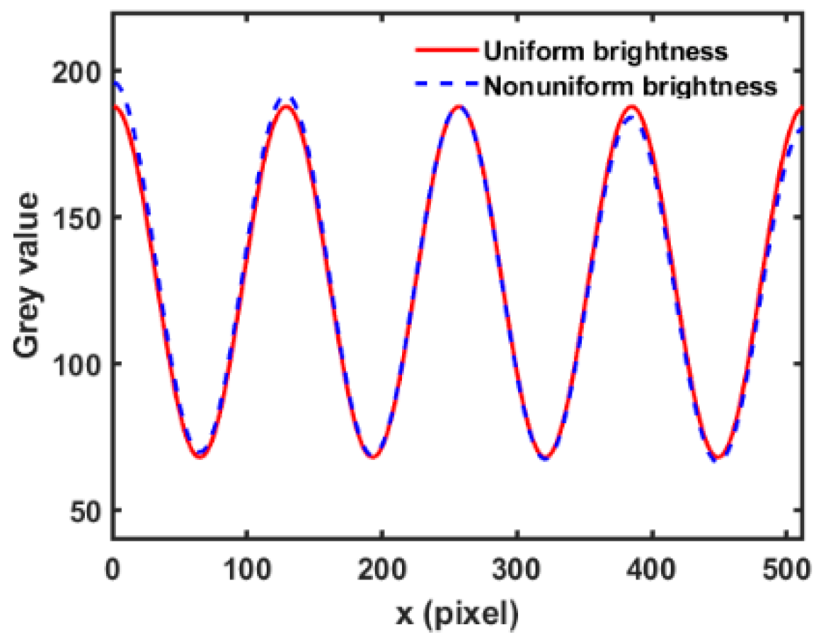
It is immunity from the non-uniform brightness distribution caused by the environment or by the lens distortion because the optical flow is calculated point-by-point.

2. Principles

2.1. Brox Optical Flow Estimation Algorithm

Define the first image to be at time t and the second image at $t+\mathrm{\Delta }t$. The point $A\left(x_i,y_i\right)$ of the gray value $I\left(x_i,y_i,t\right)$ in the first image moves to the point $B\left(x_i+\mathrm{\Delta }{x}_i,y_i+\mathrm{\Delta }{y}_i\right)$ of the gray value $I\left(x_i+\mathrm{\Delta }{x}_i,y_i+\mathrm{\Delta }{y}_i,t+\mathrm{\Delta }t\right)$ in the second image, where $\mathrm{\Delta }{x}_i$ and $\mathrm{\Delta }{y}_i$ represent the displacement components of the point $A\left(x_i,y_i\right)$ in the x and y directions, respectively. According to the assumption of constant brightness, we have the expression as follows.

$$I\left(x_i,y_i,t\right)=I\left(x_i+\mathrm{\Delta }{x}_i,y_i+\mathrm{\Delta }{y}_i,t+\mathrm{\Delta }t\right)$$

(1)

Expand the right item in Equation (1) by Taylor expansion and neglect its higher-order items, then obtain the fundamental equation of optical flow as Equation (2).

$$I_{xi}u+I_{yi}v=-I_{ti}$$

(2)

where $I_{xi}$, $I_{yi}$, and $I_{ti}$ are the partial derivatives of I with respect to $x_i$, $y_i$, and t, respectively. $u=\mathrm{\Delta }{x}_i/\mathrm{\Delta }t$ and $v=\mathrm{\Delta }{y}_i/\mathrm{\Delta }t$, are the velocity components in the x and y directions. Note that this equation is an indeterminate equation with two unknowns, u and v. Hence, additional constraints are required to estimate the velocity field $\left(u,v\right)$. The additional constraints in the Brox algorithm are the assumption of constant brightness and the assumption of constant image gradient, which are realized by constructing an energy function as follows.

$$\begin{array}{l}E\left(u,v\right)={\displaystyle \underset{\mathrm{\Omega }}{\mathrm{\int }}\psi \left[{\left|I\left(x_i+u,y_i+v\right)-I\left(x_i,y_i\right)\right|}^2+\beta {\left|\nabla I\left(x_i+u,y_i+v\right)-\nabla I\left(x_i,y_i\right)\right|}^2\right]d{x}_{i}d{y}_i}\\ +\alpha {\displaystyle \underset{\mathrm{\Omega }}{\mathrm{\int }}\psi \left({\left|\nabla u\right|}^2+{\left|\nabla v\right|}^2\right)d{x}_{i}d{y}_i}\end{array}$$

(3)

where $\left(x_i,y_i\right)$ represents the coordinates of pixel points in the image. $\mathrm{\Omega }$ represents the image domain and $\left(x_i,y_i\right)\in \mathrm{\Omega }$. $I\left(·\right)$ denotes the light intensity, $\nabla$ the gradient operator, $\beta$ the weight coefficient, and $\alpha$ the smoothing factor. $u\left(x_i,y_i\right)$ and $v\left(x_i,y_i\right)$ represent the optical flow field between the two images. The function $\psi \left(x_i{}^2\right)=\sqrt{x_i{}^2+{\epsilon }^2}$ is introduced to reduce the impact of outliers in the quadratic term on the estimate of the optical flow. In Equation (3), the first integral term stands for the data term, and the second integral term represents the smooth term. Since the Brox algorithm requires the optical flow field to be as smooth as possible, it uses the variational method to obtain the minimum value of Equation (3), and the corresponding Euler-Lagrange equation is:

$$\begin{gathered} {\mathrm{\Psi }}^{\prime }\left(I_z^2\right)I_x{I}_z+\beta {\mathrm{\Psi }}^{\prime }\left(I_{xz}^2+I_{yz}^2\right)\left(I_{xx}{I}_{xz}+I_{xy}{I}_{yz}\right)-\alpha div\left[{\mathrm{\Psi }}^{\prime }\left(u_x^2+u_y^2+v_x^2+v_y^2\right)\left(u_x{\stackrel{\rightharpoonup }{e}}_x+u_y{\stackrel{\rightharpoonup }{e}}_y\right)\right]=0 \\ {\mathrm{\Psi }}^{\prime }\left(I_z^2\right)I_y{I}_z+\beta {\mathrm{\Psi }}^{\prime }\left(I_{xz}^2+I_{yz}^2\right)\left(I_{xy}{I}_{xz}+I_{yy}{I}_{yz}\right)-\alpha div\left[{\mathrm{\Psi }}^{\prime }\left(u_x^2+u_y^2+v_x^2+v_y^2\right)\left(v_x{\stackrel{\rightharpoonup }{e}}_x+v_y{\stackrel{\rightharpoonup }{e}}_y\right)\right]=0 \end{gathered}$$

(4)

where $div\left(·\right)$ denotes the divergence operator, ${\mathrm{\Psi }}^{\prime }\left(x_i{}^2\right)=\frac{1}{2\sqrt{x_i{}^2+{\epsilon }^2}}$, $u_x=\frac{\partial u}{\partial x_i}$, $u_y=\frac{\partial u}{\partial y_i}$, $v_x=\frac{\partial v}{\partial x_i}$, $v_y=\frac{\partial v}{\partial y_i}$. ${\stackrel{\rightharpoonup }{e}}_x$ and ${\stackrel{\rightharpoonup }{e}}_y$ are the unit vectors in the x and y directions, respectively. $I_x=\frac{\partial I\left(x_i+u,y_i+v\right)}{\partial x_i}$, $I_y=\frac{\partial I\left(x_i+u,y_i+v\right)}{\partial y_i}$, $I_z=I\left(x_i+u,y_i+v\right)-I\left(x_i,y_i\right)$, $I_{xx}=\frac{{\partial }^{2}I\left(x_i+u,y_i+v\right)}{\partial x_i{}^2}$, $I_{xy}=\frac{{\partial }^{2}I\left(x_i+u,y_i+v\right)}{\partial x_i\partial y_i}$, $I_{yy}=\frac{{\partial }^{2}I\left(x_i+u,y_i+v\right)}{\partial y_i{}^2}$, $I_{xz}=\frac{\partial I\left(x_i+u,y_i+v\right)}{\partial x_i}-\frac{\partial I\left(x_i,y_i\right)}{\partial x_i}$ and $I_{yz}=\frac{\partial I\left(x_i+u,y_i+v\right)}{\partial y_i}-\frac{\partial I\left(x_i,y_i\right)}{\partial y_i}$.

For a detailed derivation of Equation (4), please refer to reference [22]. The differentials in Equation (4) are discretized, and the image optical flow vector can be obtained by using the SOR iteration. More information can be found in references [20,22]. Then, the displacement of the point $A\left(x_i,y_i\right)$ can be obtained, that is $\mathrm{\Delta }{x}_i=u$ and $\mathrm{\Delta }{y}_i=v$, when we set the time interval between two images as 1. Meanwhile, the displacement of the corresponding point $A\left(x,y\right)$ on the reference plane can be expressed as $\mathrm{\Delta }x=\mathrm{\Delta }{x}_i/M_c$ and $\mathrm{\Delta }y=\mathrm{\Delta }{y}_i/M_c$, where $M_c$ represents the magnification of the camera.

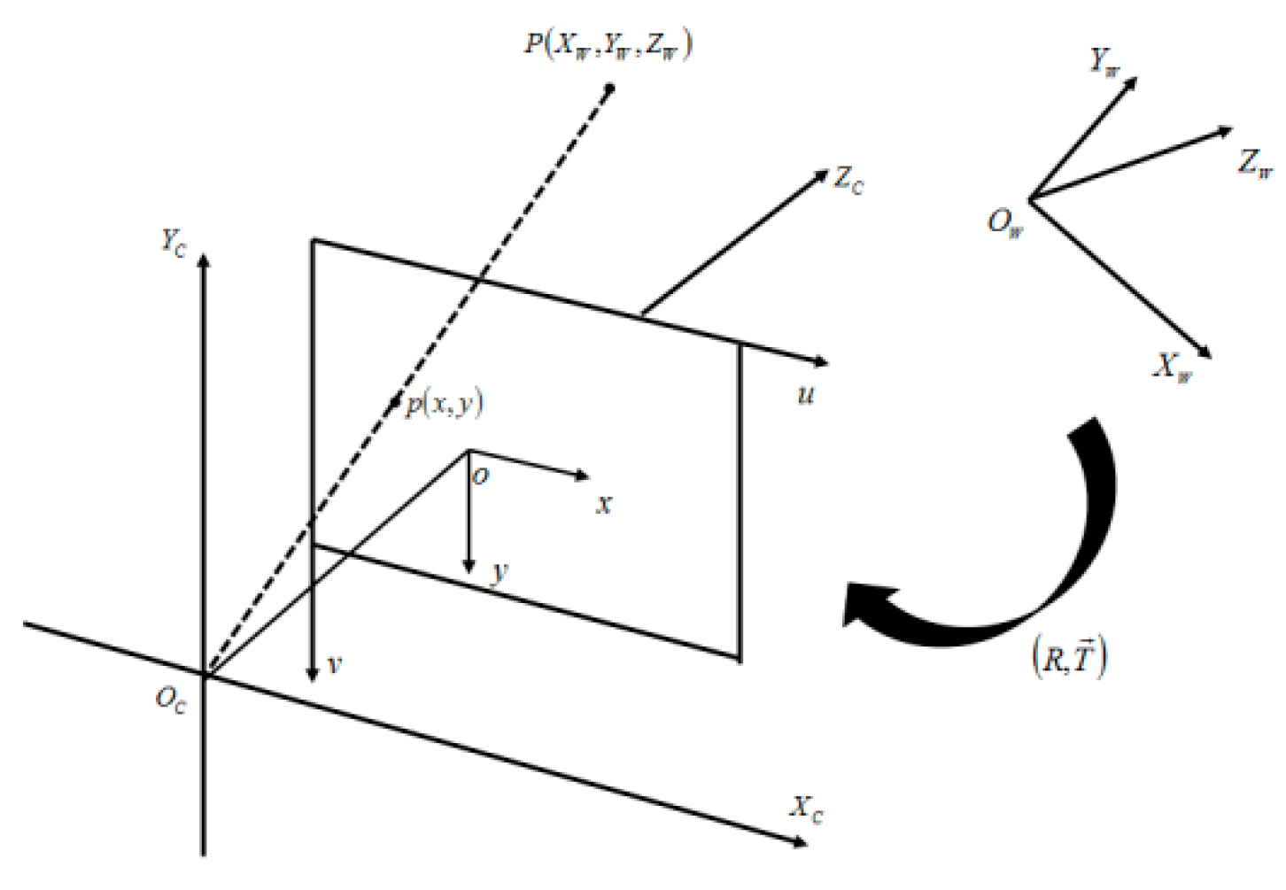
2.2. Principle of Camera Calibration

Figure 1 shows the pin-hole model of a single camera. The model describes the relationship between the world coordinate system $\left(O_W-X_W{Y}_W{Z}_W\right)$, the camera coordinate system $\left(O_C-X_C{Y}_C{Z}_C\right)$, and the image coordinate system $\left(o-xy\right)$. As shown in Figure 1, $u-v$ represents the pixel coordinate system, whose origin is located in the upper left corner of the image. The rotation matrix R and the translation matrix $\overrightarrow{T}$ constitute the external parameter matrix of the camera, which describes the transformation between the world coordinate system and the camera coordinate system. The internal parameter matrix consists of the focal length $f$ of the camera, distortion factor $\gamma$, and the coordinate of the principal point, which represents the transformation between the camera coordinate system and the image coordinate system. $P\left(X_W{Y}_W{Z}_W\right)$ is a point in the world coordinate system. Then, the camera pin-hole model can be mathematically expressed as:

Figure 1. Camera pin-hole model.

Figure 1. Camera pin-hole model.

$$s\left[\begin{array}{c}u\\ v\\ 1\end{array}\right]=\left[\begin{array}{ccc}{f}_u& \gamma & u_0\\ 0& f_v& v_0\\ 0& 0& 1\end{array}\right]\left[\begin{array}{cc}R& \overrightarrow{T}\end{array}\right]\left[\begin{array}{c}{X}_W\\ Y_W\\ Z_W\\ 1\end{array}\right]$$

(5)

where s is the scale factor, $\gamma$ is the distortion factor. $f_u$ and $f_v$ represent the focal length of the camera along u and v directions, respectively. $\left(u_0,v_0\right)$ denotes the coordinate of the principal point. The translation matrix $\overrightarrow{T}$ and the rotation matrix R can be expressed as

$$T=\left(\begin{array}{l}{t}_x\\ t_y\\ t_z\end{array}\right),R=\left(\begin{array}{ccc}\cos {\theta }_3& \sin {\theta }_3& 0\\ -\sin {\theta }_3& \cos {\theta }_3& 0\\ 0& 0& 1\end{array}\right)\left(\begin{array}{ccc}\cos {\theta }_2& 0& -\sin {\theta }_2\\ 0& 1& 0\\ \sin {\theta }_2& 0& \cos {\theta }_2\end{array}\right)\left(\begin{array}{ccc}1& 0& 0\\ 0& \cos {\theta }_1& \sin {\theta }_1\\ 0& -\sin {\theta }_1& \cos {\theta }_1\end{array}\right)$$

where $t_x$, $t_y$, and $t_z$ denote the translation components of the world coordinate system in x, y, and z directions to the camera coordinate system, respectively. These translation components are $x_c$, $y_c$, and $z_c$, the three coordinate components of the camera in the world coordinate system. ${\theta }_1$, ${\theta }_2$, and ${\theta }_3$ are the rotation angles of the world coordinate system rotating about x, y, and z axes to the camera coordinate system, respectively. Usually, employ a board printed with uniformly distributed grids as the calibration plate to calibrate the camera. The intersections of the grid are taken as feature points. Record a series of images of the calibration plate at different positions, generally about 20 images, to achieve high accuracy [5], by which the coordinates of feature points in each image can be extracted. Based on the information on these feature points, the parameter matrix in Equation (5) can be determined by using the least square method. We complete the calibration of the camera with the MATLAB camera calibration toolbox in this work.

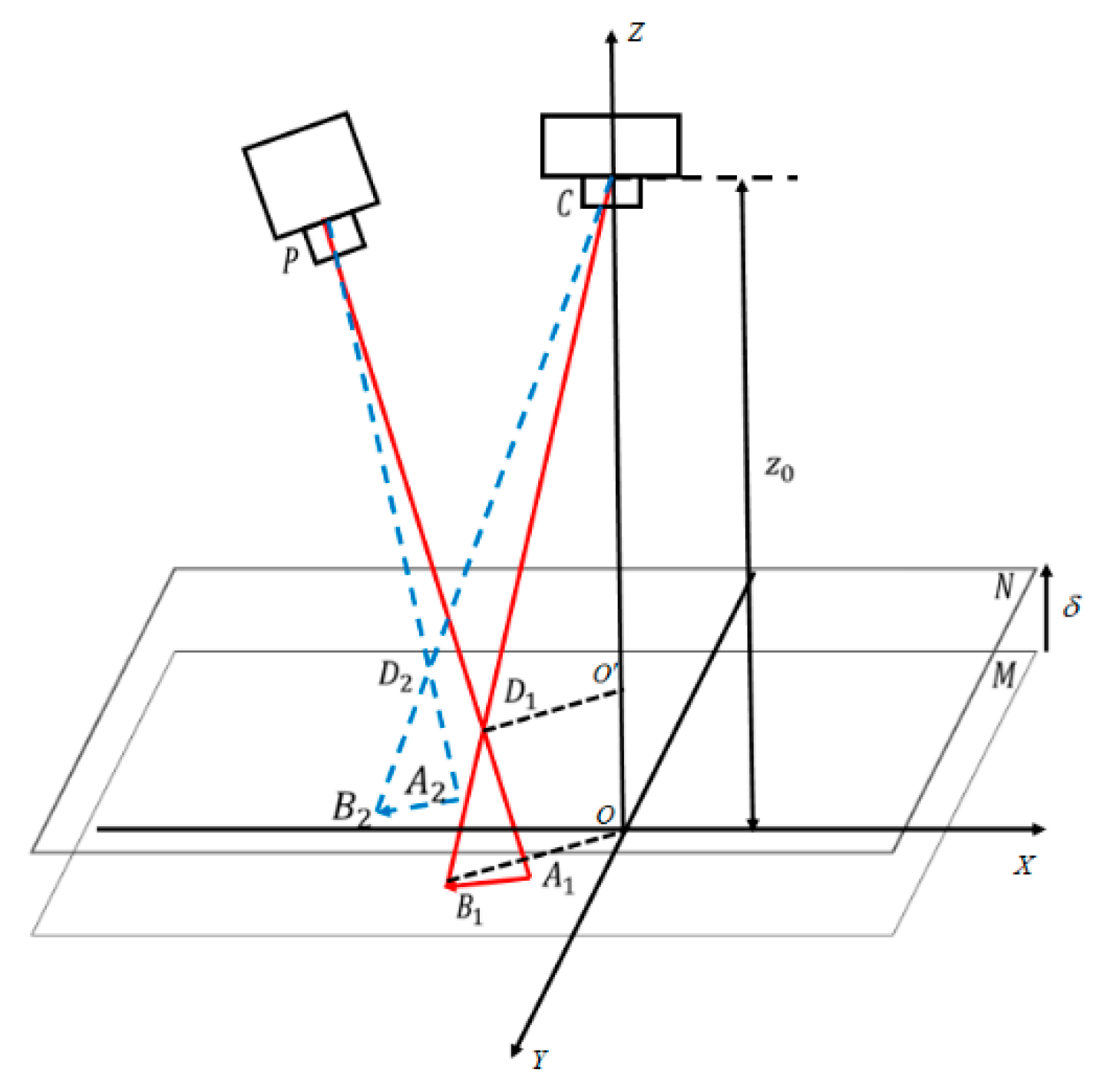
2.3. Principle of Projector Calibration

As shown in Figure 2, the calibration tool is a calibration plate except for the projector and the camera, which is fixed on a moving platform driven by a computer-controlled stepper motor to achieve precise displacement. The origin place of the calibration plate is located at plane M, taken as the reference plane. Point C represents the optical center of the camera, and CO is a line perpendicular to plane M. Point O is taken as the origin of the coordinate system. Note that the image distance CO is $z_0$, obtained by calibrating the camera in Section 2.2.

Then, the coordinate of point C is $\left(0,0,z_0\right)$. Let the coordinate of projector P be $\left(x_p,y_p,z_p\right)$. Move the calibration plate a distance $\delta$ upwards to a new place N, the z-axis intersects plane N at a new intersection point $O^{\prime }$. Consider that a beam radiates from the projector to point $A_1\left(x_{A1},y_{A1},0\right)$ on plane M. The projection line $P{A}_1$ intersects the plane N at point $D_1\left(x_{D1},y_{D1},\delta \right)$, which has the same gray value as point $A_1$. When observing point $D_1\left(x_{D1},y_{D1},\delta \right)$ at the location of the camera, we find its corresponding point $B_1$ on the reference surface M. $A_1{B}_1$ represents the displacement resulting from the shift of the calibration plate, which can be estimated by the optical flow method. Then, the location of point $B_1$ can be obtained, that is $x_{B1}=x_{A1}+\mathrm{\Delta }x$, $y_{B1}=y_{A1}+\mathrm{\Delta }y$, where $\mathrm{\Delta }x$ and $\mathrm{\Delta }y$ are the displacement components of the point $B_1$. $\mathrm{\Delta }x=M_c\cdot u$, $\mathrm{\Delta }y=M_c\cdot v$, where u and v are the optical flow in the x and y directions, respectively, and $M_c$ represents the magnification of the camera. After the camera calibration is completed and further the optical flow fields caused by the translation of the calibration plate are calculated, then, the coordinates of point $D_1$ can be obtained based on the similarity between $\mathrm{\Delta }C{D}_1{O}^{\prime }$ and $\mathrm{\Delta }C{B}_{1}O$. The expression is as follows.

$$\begin{gathered} x_{D1}=\frac{z_0-\delta }{z_0}\cdot x_{B1}=\frac{z_0-\delta }{z_0}\cdot \left(x_{A1}+M_c\cdot u\right) \\ {y}_{D1}=\frac{z_0-\delta }{z_0}\cdot y_{B1}=\frac{z_0-\delta }{z_0}\cdot \left(y_{A1}+M_c\cdot v\right) \\ {z}_{D1}=\delta \end{gathered}$$

(6)

The line $A_1{D}_1$ can be expressed as

$$\frac{x-x_{A1}}{x_{D1}-x_{A1}}=\frac{y-y_{A1}}{y_{D1}-y_{A1}}=\frac{z}{\delta }$$

(7)

Obviously, the position of the projector must be located on the line $A_1{D}_1$. Once another equation of projection line $A_2{D}_2$ is obtained, the projector position P can be derived by the intersection point of the two lines. The line $A_2{D}_2$ can be expressed as

$$\frac{x-x_{A2}}{x_{D2}-x_{A2}}=\frac{y-y_{A2}}{y_{D2}-y_{A2}}=\frac{z}{\delta }$$

(8)

From Equations (7) and (8), we can obtain the coordinates of point P.

$$\begin{gathered} x_p=\frac{x_{A1}\left(x_{D2}-x_{A2}\right)-x_{A2}\left(x_{D1}-x_{A1}\right)}{\left(x_{D2}-x_{A2}\right)-\left(x_{D1}-x_{A1}\right)} \\ {y}_p=\frac{y_{A1}\left(y_{D2}-y_{A2}\right)-y_{A2}\left(y_{D1}-y_{A1}\right)}{\left(y_{D2}-y_{A2}\right)-\left(y_{D1}-y_{A1}\right)} \\ {z}_p=\delta \cdot \frac{x_p-x_{A1}}{x_{D1}-x_{A1}} \end{gathered}$$

(9)

Assume that the captured images are of the size of $p\times q$. As a way to improve the accuracy, two intersecting lines $A_i{D}_i$ and $A_j{D}_j$ in n groups are taken, and their intersection points are calculated. Then, Equation (9) can be rewritten as

$$\begin{gathered} x_{p_i}=\frac{x_{A_i}\left(x_{D_j}-x_{A_j}\right)-x_{A_j}\left(x_{D_i}-x_{A_i}\right)}{\left(x_{D_j}-x_{A_j}\right)-\left(x_{D_i}-x_{A_i}\right)} \\ {y}_{p_i}=\frac{y_{A_i}\left(y_{D_j}-y_{A_j}\right)-y_{A_j}\left(y_{D_i}-y_{A_i}\right)}{\left(y_{D_j}-y_{A_j}\right)-\left(y_{D_i}-y_{A_i}\right)} \\ {z}_{p_i}=\delta \cdot \frac{x_{p_i}-x_{A_i}}{x_{D_i}-x_{A_i}} \end{gathered}$$

(10)

where $n=1,2,\cdots ,\left(p\times q-1\right)!$, $i,j=1,2,\cdots ,p\times q$, and $i\ne j$. Finally, three coordinates at point P can be calculated by $\left(\frac{{\displaystyle \sum _{i=1}^n{x}_{p_i}}}{n},\frac{{\displaystyle \sum _{i=1}^n{y}_{p_i}}}{n},\frac{{\displaystyle \sum _{i=1}^n{z}_{p_i}}}{n}\right)\left[n=1,2,\cdots ,\left(p\times q-1\right)!\right]$.

Although only two images are used for projector calibration, all pixels in the captured images can be used as effective information points, by which the projector calibration is of high accuracy. By using the calibrated coordinates of the camera and the projector, the height distribution of a measured object can be obtained efficiently [23,24].

3. Numerical Simulations

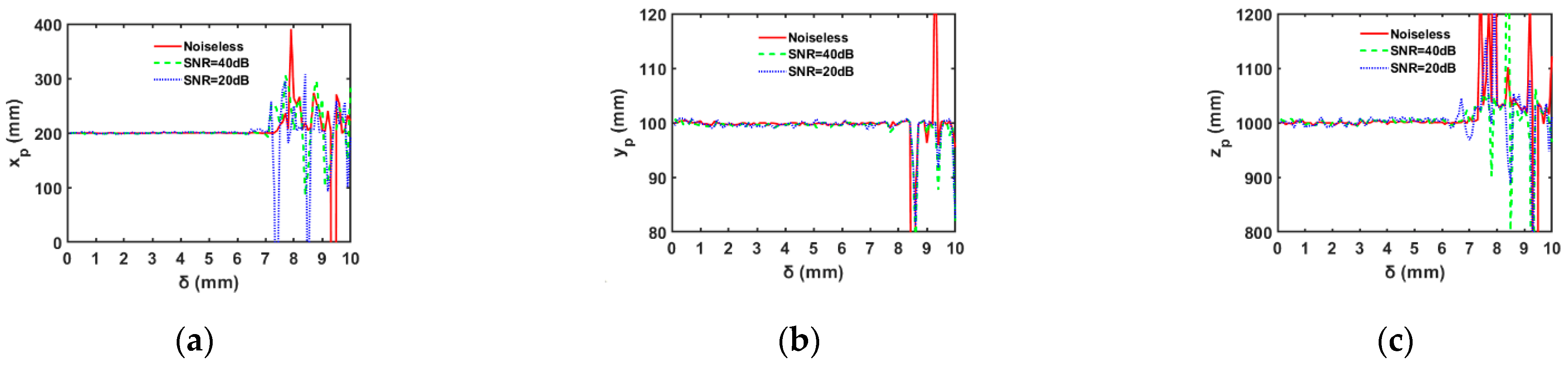
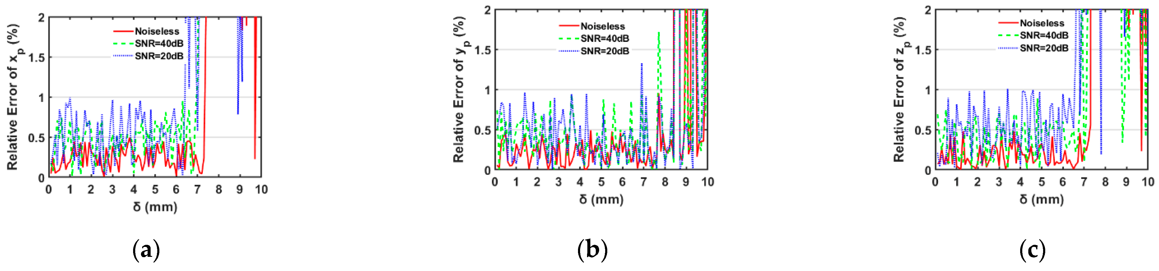
3.1. Range Estimation of Moving Distance of Calibration Plate

In a two-dimensional coordinate system, Figure 2 can be represented by Figure 3. Assume that the projector is located at the same height as the camera. Note that $\mathrm{\Delta }x$ increases with the increase of $\delta$, so as to $\mathrm{\Delta }{x}_i$, the displacement component in the x direction on the image plane. However, optical flow methods are suitable for small displacement measurements [19,20,21]. Therefore, it is necessary to limit the displacement of the calibration plate to ensure accuracy. It can be seen from Figure 3 that:

$$\mathrm{\Delta }x=\frac{\delta d}{z_c-\delta }$$

(11)

where d is the horizontal distance between the projector and the camera, and $z_c$ is the image distance of the camera. In Section 2.1, we have found that $\mathrm{\Delta }{x}_i=\mathrm{\Delta }x\cdot M_c$. It is assumed that the minimum and maximum displacements that the Brox algorithm can detect are $\mathrm{\Delta }{x}_{i\min }$ and $\mathrm{\Delta }{x}_{i\max }$, respectively. They should satisfy the relation that is $\mathrm{\Delta }{x}_{i\min }<\mathrm{\Delta }{x}_i<\mathrm{\Delta }{x}_{i\max }$, namely, $\mathrm{\Delta }{x}_{i\min }/M_c<\mathrm{\Delta }x<\mathrm{\Delta }{x}_{i\max }/M_c$. Then, we can derive the range of $\delta$ as

$$\frac{z_c\mathrm{\Delta }{x}_{i\min }/M_c}{d+\mathrm{\Delta }{x}_{i\min }/M_c}<\delta <\frac{z_c\mathrm{\Delta }{x}_{i\max }/M_c}{d+\mathrm{\Delta }{x}_{i\max }/M_c}$$

(12)

According to Equation (12), as long as the minimum and maximum displacements can be detected by the Brox algorithm, the appropriate motion distance of the calibration plate can be estimated because the horizontal distance d and the image distance $z_c$ are estimated before calibration. The detected minimum and maximum displacements represent the measurable range of the Brox algorithm. However, the discussion of the measurable range of the optical flow algorithm is a very complex work that needs to consider the frequency and size of the recorded images, camera resolution, and the parameters of the optical flow algorithm itself [18]. Here we briefly introduce it to meet the requirements of our calibration method. The detailed discussion will be introduced in our future work.

The measurable minimum and maximum displacements between two images are denoted by $\mathrm{\Delta }{x}_{i\min }$ and $\mathrm{\Delta }{x}_{i\max }$, respectively. $\mathrm{\Delta }{x}_{i\min }$ also indicates the displacement resolution of the used algorithm, sensitive to the gray levels of the image and the algorithm used to calculate optical flow. Theoretical displacement resolution can be expressed as $1/(2^m-1)$ for the images filmed with an m-bit intensity depth camera and the displacement calculated by subpixel-based algorithm [19]. However, it can be found that the theoretical resolution is not accurate. We utilize the simulation method to determine $\mathrm{\Delta }{x}_{i\min }$ and $\mathrm{\Delta }{x}_{i\max }$.

First, simulate an image with an 8-bit gray-scale level of the size of $512\times 512$ pixels, used as the original one shown in Figure 4a. The fringe frequency of the fringe pattern is 0.1 ${\mathrm{mm}}^{-1}$, parallel to the y-direction. Then, translate it to a given displacement $\mathrm{\Delta }{x}_g$ in the x-direction to produce the deformed pattern, as shown in Figure 4b. Finally, employ the original and the deformed pattern to calculate the displacement at each pixel by the Brox algorithm. The calculated value $\mathrm{\Delta }{x}_c$ is uniform due to the translation of the fringes except for the edges of the image. The accuracy of the measurement is evaluated using the relative error, defined as $\left|\mathrm{\Delta }{x}_c-\mathrm{\Delta }{x}_g\right|/\mathrm{\Delta }{x}_g$. The given displacement $\mathrm{\Delta }{x}_g$ is changed to find the minimum and maximum that the Brox algorithm can measure. When the given displacement $\mathrm{\Delta }{x}_g$ varies from $8.1\times {10}^{-6}$ to $9.0\times {10}^{-6}$ pixels, the relative error of the calculated displacement decreases with the increase of the displacement, as shown in Figure 5a. It can be found that the measurable minimum is $8.3\times {10}^{-6}$ pixel when the relative error is required to be less than 0.5%. When the given displacement $\mathrm{\Delta }{x}_g$ varies from 11 to 20 pixels, the relative error of the calculated value increases with the increase of the displacement, as shown in Figure 5b. The measurable maximum is 19 pixels when the relative error is required less than 0.5%. In this work, the smoothing factor $\alpha$ in the Brox algorithm is 100, and the weight coefficient $\beta$ is 10. To summarize these sentences above, the displacement range from $8.3\times {10}^{-6}$ to 19 pixels can be detected by the Brox algorithm when the relative error is less than 0.5%.

Knowing the measurable displacement of the Brox algorithm, we can set the simulation experiment parameters according to the actual experimental arrangement. Set the image distance $z_c$ as 1000 mm and the magnification factor $M_c$ as $512/40$ pixel/mm. The horizontal distance between the projector and the camera d is 200 mm. According to Equation (12), the appropriate displacement $\delta$ of the calibration plate is estimated as 7 mm, using the maximum measurable displacement of 19 pixels. In Section 3.2, the displacement of the calibration plate is also set in the range of 7 mm.

3.2. Projector Calibration

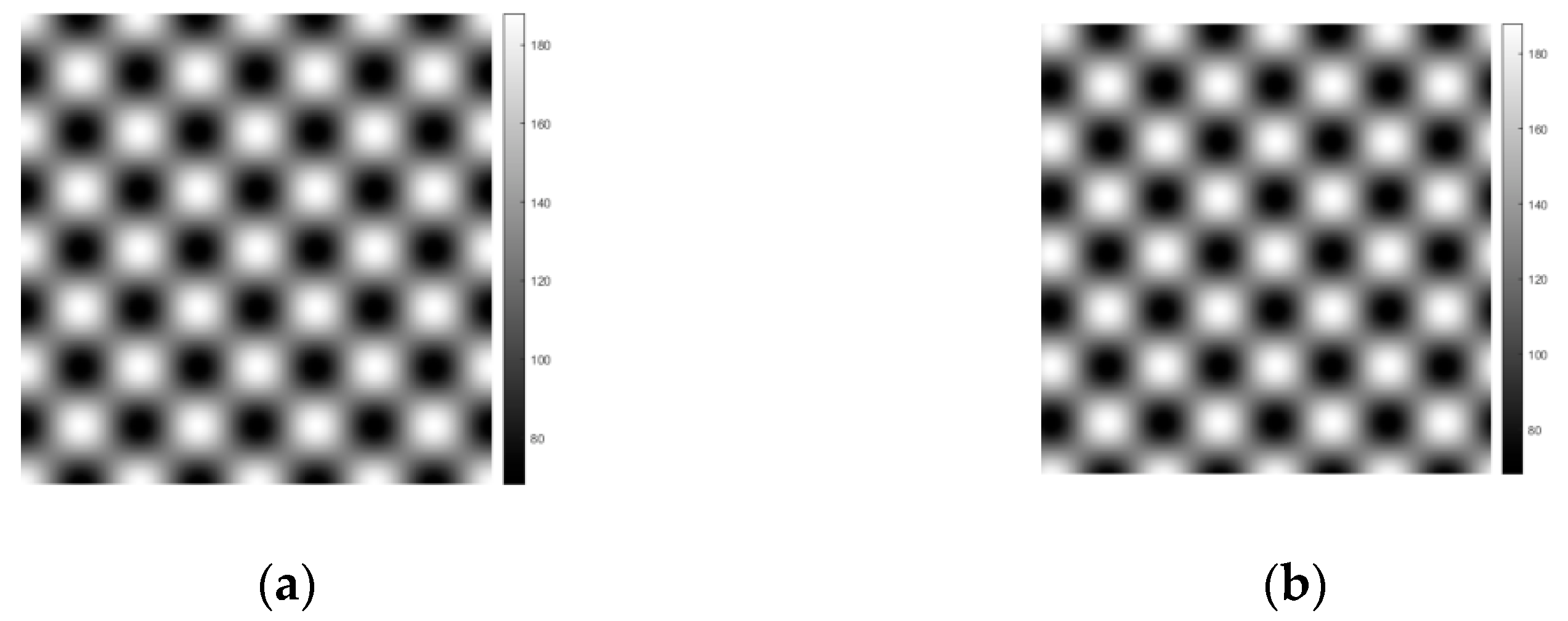
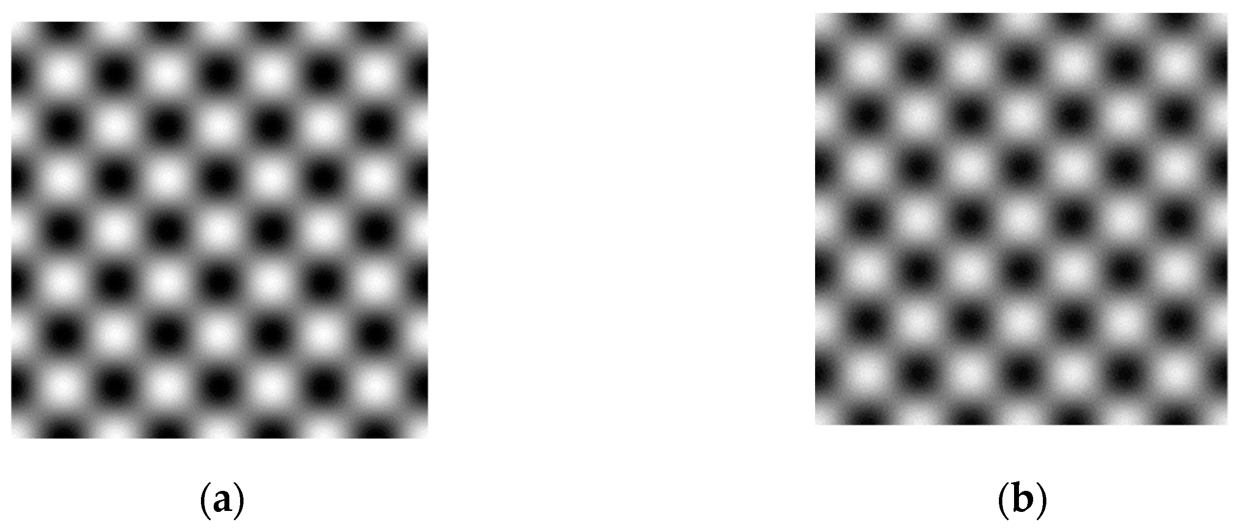
3.2.1. Projector Calibration with Uniform Brightness Pattern

Since the optical flow is sensitive to the displacement in the direction of the gray gradient, we utilize a grid pattern with sine grayscale distribution in the x and y direction to perform the calibration. The projected grid pattern is of uniform brightness, expressed by Equation (13).

$$I=a+b\cos \left(2\pi f_{x}x\right)\cos \left(2\pi f_{y}y\right)$$

(13)

where a is the background light intensity, and b is the fringe contrast. $f_x$ and $f_y$ are the local frequency in the x and y directions, respectively. Define a as 128, and b as 60, $f_x$ equal to $f_y$, is 0.1 mm⁻¹. The grid pattern shown in Figure 6a is used as the projection pattern before movement. Then, move the calibration plate a distance of 7 mm toward the camera, i.e., $\delta =7$ mm. The captured pattern after movement is shown in Figure 6b. The size of the images in Figure 6 is 512 × 512 pixels.

It is necessary to calibrate the three coordinates of the projector simultaneously in the optical flow method. As the main system parameters to be calibrated, the three coordinate components of the projector and the coordinate components of the camera, we set them in the simulation according to the actual experimental arrangement. As shown in Figure 2, the image distance $z_c$ is set as 1000 mm. The projector is set at a given point $(x_g,y_g,z_g)$, that is (200, 100, 1000), where the unit is mm. The magnification $M_c$ is set as $512/40$ pixel/mm, which illustrates that the measured object is the size of 40 × 40 mm, and the size of the captured images is 512 × 512 pixels. In order to reduce computational time and avoid the edge effects existing in the calculations, the data used to calibrate the projector would be confined to an area that is 100 pixels smaller than the size of the captured images. Then, the optical flow at each pixel within the area of 400 × 400 pixels in the images is used as the effective information. Three coordinate components of the projector can be determined by Equation (10) using the two images before and after the movement of the calibration plate, represented by ($x_p,y_p,z_p$), that is (200.33, 100.05, 1003.78). The corresponding relative error of the three components is 0.17%, 0.05%, and 0.38%, respectively.

3.2.2. Projector Calibration with Non-Uniform Brightness Pattern

However, in the actual experiment, the brightness on the reference plane is not uniform due to the tilted projection, which may affect the calibration results.

As shown in Figure 7, points P and C represent the locations of the optical center of the projector and the camera, respectively. $\theta$ represents the incident angle of the projector, the angle between the optical axis of the projector PO, and that of the camera OC. Point O is the origin of the coordinate system. r represents the length of a projection line PA, and $r_0$ represents the length of the projection line PO. A(x, 0) is an arbitrary point on the reference plane M. With the same brightness as point A, point D is the intersection of the projection line PA with plane N, the calibration plate located after movement.

The oblique projection may cause brightness problems in several ways, as follows. First, we assume that all points on the same ray have the same intensity of light. In fact, the intensity of light at points along the projection line varies with the propagation distance according to the inverse square law of brightness. The light transmitted from the projector has a brightness of $I_r$ after a distance r. Then, we have

$$I_r\propto 1/r^2$$

(14)

where $r^2=x^2+r_0^2-2xd$. Therefore, there is a small brightness difference between point A and point D. However, it is too small to be ignored because the moving displacement $\delta$ is small.

Second, the tilting projection makes the brightness uneven on the calibration plate. The brightness of point A is different from that of point $A^{\prime }$. Define $I_0$ as the light intensity at propagation distance $r_0$, represents the uniform brightness distribution on the reference plane and has the expression as Equation (13). The brightness distribution on reference plane M can be expressed as

$$I_r=\frac{r_0^2\cdot I_0}{x^2-2dx+r_0^2}$$

(15)

According to Equation (15), we simulate the brightness distribution on the reference plane. The result is shown in Figure 8, which shows the comparison between the uniform and non-uniform brightness distribution on the cross-section at 256 pixels in the y-direction. There are slight differences between them. Subsequently, using the two images to calibrate the projector in the same parameters as that in Section 3.2.1, we obtain three coordinate components of the projector, which are 200.35 mm, 99.79 mm, and 1004.61 mm in x, y, and z-direction, respectively. Compared with their true values, the relative error of the three components is 0.18%, 0.21%, and 0.46%, respectively. Compared with the error in uniform brightness distribution shown in Section 3.2.1, the error changes slightly under the non-uniform brightness distribution due to oblique illumination. Non-uniform brightness distribution has little effect on the calibration results. The reason is that the optical flow method performs to search for the corresponding point of the same brightness in a small local area for displacement measurement.

3.3. Discussion of the Calibration

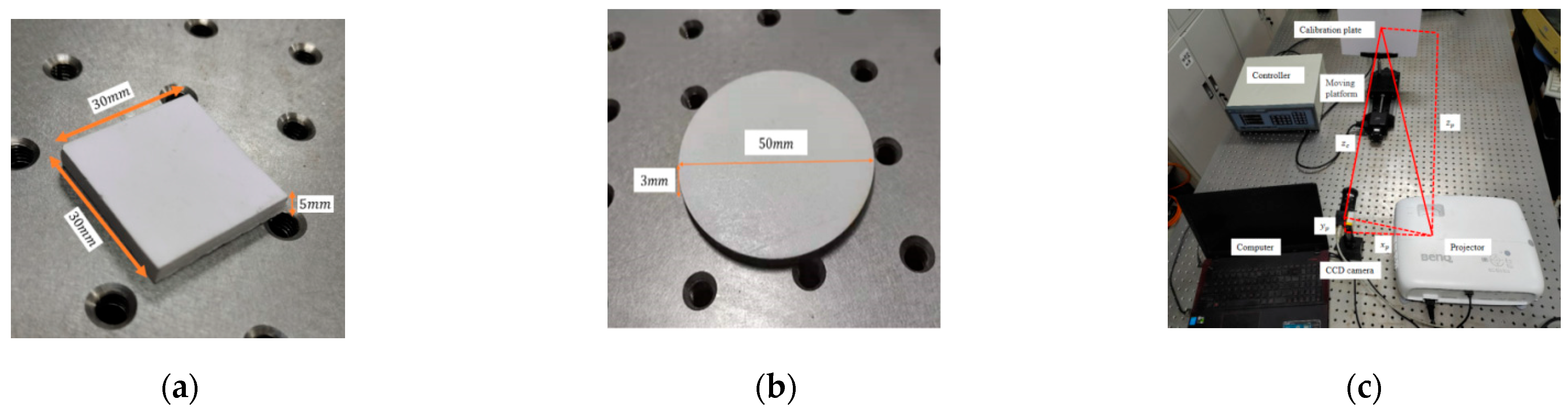
In the actual measurement, the accuracy of the proposed method is mainly disturbed by the environmental noise, the moving range of the calibration plate, the mechanical error of the moving platform, the calibration error of the camera, and the calculation error of the optical flow. Among these factors, the calculation error of the optical flow is small according to the contribution [18]. Therefore, in this section, we discuss the influence of these remaining factors on calibration.

Firstly, we analyze the influence of the moving distance of the calibration plate on the calibration result when the projector is located at the given position. Meanwhile, to show the influence of noise, the images shown in Figure 6 are polluted by Gaussian noise of SNR of 40 dB and 20 dB, respectively. The noised images are shown in Figure 9a,b, respectively. According to Equation (12), the allowable movement range of the calibration plate, which is from $8.3\times {10}^{-6}$ to 7 mm, is in the absence of noise when the projector locates at the point (200, 100, 1000) mm. However, it is not appropriate for the calibration plate to move too little in the actual measurement because of the mechanical error of the moving platform. Therefore, we selected the moving distance of the calibration plate in the range of 0.1 mm to 10 mm with a step of 0.1 mm.

Use the image before the movement as the first one and the image after the movement as the second to calculate the projector’s location, according to Equation (10). The results are the three coordinate components in the x, y, and z directions, illustrated in Figure 10a–c, respectively, showing the variation of the component $\delta$ under different noise levels. It can be found that the calculated coordinate components are very close to their given value with a small fluctuation in the range from 0 about to 7.0 mm in the x, y, and z direction. The distributions of their relative error, as shown in Figure 11, reveal the accuracy of the calibration results more clearly. The relative errors are less than 0.5% in the x, y, and z directions when the movement distance is between 0 and 7.3 mm in the absence of noise. The noise increases the measurement error and decreases the movable range of the calibration plate. The relative errors are less than 0.8% in the x, y, and z directions when the images are with the noise of SNR of 40 dB, corresponding to the movement range of 0 to 7.0 mm. Further, when the images are polluted by the noise of SNR of 20 dB, the relative errors are less than 1.0% in the x, y, and z directions with the calibration plate movable range of 0 to 6.5 mm. It is obvious that the calibration results are still of high accuracy when the SNR of the images is 20 dB, which shows that the proposed method has good robustness to noise. In the actual measurement, the noise level of the images is generally below 20 dB. Then we can obtain an advisable movement range of the calibration plate, which is within 6.5 mm, in an actual experiment. However, in practical application, we should choose as large a value as possible within this range to reduce the influence of the calibration plate motion error.

Then, the positioning error of the camera introduced by the camera calibration, and the positioning error of the calibration plate, including the thread pitch and thread clearance in the moving platform, will inevitably affect calibration accuracy. Therefore, it is necessary to analyze their impacts on the calibration results.

Similar to the simulation in Section 3.2.1, set the projector coordinates first. Then, assign the imaging distance and the displacement of the calibration plate with possible errors. Use these selected parameters to generate images before and after deformation. Finally, estimate the coordinate value of the projector using the two images, and calculate the error of the calculated value.

Set $(x_g,y_g,z_g)$, the location of the projector as (200, 100, 1000), where the unit is mm. Set $z_c$ as 1000 mm, the image distance with the calibration error of 5 mm, i.e., $z_c=1000\pm 5$ mm. In addition, set $\delta$ as 7 mm, the moving distance of the calibration plate with an error of 0.1 mm in the noiseless case, i.e., $\delta =7\pm 0.1$ mm. Obviously, these errors are deliberately set large in order to see how they affect the calibration results. According to the size of the setting errors, the image distance $z_c$ could be anything in the range from 995 mm to 1005 mm and the moving distance of the calibration plate, $\delta$, in the range from 6.9 mm to 7.1 mm.

We divide these parameters into the four cases, shown in

Table 1. The influence of camera calibration error and calibration plate movement error on the results.

${\mathit{z}}_{\mathit{c}}/\mathit{\delta }\left(\mathbf{mm}\right)$	${\mathit{x}}_{\mathit{p}}\left(\mathbf{mm}\right)$	${\mathit{x}}_{\mathit{p}}$ Relative Error (%)	${\mathit{y}}_{\mathit{p}}\left(\mathbf{mm}\right)$	${\mathit{y}}_{\mathit{p}}$ Relative Error (%)	${\mathit{z}}_{\mathit{p}}\left(\mathbf{mm}\right)$	${\mathit{z}}_{\mathit{p}}$ Relative Error (%)
1000.00/7.00	200.33	0.17	100.05	0.05	1003.78	0.38
1005.00/7.10	201.26	0.63	100.14	0.14	1007.12	0.71
995.00/6.90	199.34.	0.33	100.77	0.77	993.54	0.65
1005.00/6.90	198.41	0.80	100.24	0.24	991.24	0.88
995.00/7.10	202.34	1.90	100.65	0.65	1009.71	0.97

, according to their possible values. The coordinates of the projector are calculated using the possible values according to Equation (10), which are compared with that from the exact parameters, i.e., $z_c=1000$ mm and $\delta =7$ mm. It can be seen from Table 1 that the relative errors are less than 1% in most combinations. It illustrates that the positioning error of the camera and the calibration plate has a certain influence on the calibration results and will produce calibration error. Although the error is not large, it should be reduced as far as possible for precision measurement.

4. Experiment

In order to verify the effectiveness and accuracy of the proposed calibration method in this work, the eight-step phase measurement profilometry of an acknowledged high accuracy is used to measure two specimens. One is a square plate with the size of $30.00\times 30.00\times 5.00$ mm, as shown in Figure 12a. The other is a circular thin plate with a diameter of 50 mm and a thickness of 3 mm, as shown in Figure 12b. The two specimens are measured respectively by using the experiment system, shown in Figure 12c, composed of a camera, a projector, and the calibration plate fixed to a moving platform driven by a stepping motor controlled by the controller. The computer is used to select the projected pattern and process the captured image. Parameters in the calibration process include $x_p$, $y_p$, $z_p$, and $z_c$, are shown in Figure 12c. The system parameters in measuring the square plate are different from that in the circular thin plate, which is calibrated, respectively, by the proposed method and Falcao’s method [9] simultaneously. Then, calculate the height of each specimen using the parameters calibrated by the two methods for comparison.

Firstly, use the proposed method to calibrate the system according to the following steps.

1.

The camera calibration is completed to obtain the image distance $z_c$. This step can be completed by using the camera calibration toolbox with MATLAB;

2.

The grid pattern generated according to Equation (13) is projected on the calibration plate. The first image captured by the camera is shown in Figure 13a, and the plane where the calibration plate is located is defined as the reference plane;

3.

Move the platform and then capture the second image, as shown in Figure 13b, after estimating the motion range of the moving platform roughly according to Equation (12). If the calibration board moves toward the camera, the moving distance is defined as positive, and vice versa;

4.

Calculate the optical flow between two images, and then the 3-D coordinates of the projector can be obtained using Equation (10).

Figure 13. Captured calibration images, (a) before moving the calibration plate and (b) after moving the calibration plate.

Figure 13. Captured calibration images, (a) before moving the calibration plate and (b) after moving the calibration plate.

The move distance of the calibration plate in the two measurement systems is 5 mm, i.e., $\delta =5.0$ mm, an appropriate distance as discussed in Section 3. The magnification of the camera $M_c$ is 512/48 pixel/mm in the system for measuring the square plate. The three coordinate components of the camera $x_c$, $y_c$, and $z_c$ is −7.27 mm, 113.16 mm, and 1188.87 mm in the x, y, and z directions, respectively, calibrated using the camera calibration toolbox. Using the parameters above, the three coordinate components of the projector $x_p$, $y_p$, and $z_p$ can be estimated by the two captured images. The estimated results are 127.22 mm, 68.77 mm, and 1174.21 mm in the x, y, and z directions, respectively, calibrated using the proposed method. Moreover, 126.85 mm, 68.02 mm, and 1175.36 mm, in the x, y, and z directions, respectively, were calibrated using Falcao’s method.

In the system for measuring the circular thin plate, the magnification of the camera $M_c$ is 512/68 pixel/mm. The three coordinate components of the camera $x_c$, $y_c$, and $z_c$ are −12.11 mm, 145.15 mm, 1506.12 mm in the x, y, and z directions, respectively, calibrated using the camera calibration toolbox. By using the above parameters, the three coordinate components of the projector $x_p$, $y_p$, and $z_p$ also can be estimated by two captured images. The estimated result is 345.82 mm, 85.21 mm, and 1490.55 mm in the x, y, and z directions, respectively, calibrated using the proposed method. Furthermore, 344.77 mm, 85.03 mm, and 1488.47 mm, in the x, y, and z directions, respectively, were calibrated using Falcao’s method. It can be found that the calibration results from the two methods are very close to each other.

Secondly, using the parameters calibrated by our proposed method and Falcao’s method, the eight-step phase shift method is used to measure the two specimens. Of a recognized high precision, the eight-step phase shift method is utilized to retrieve the surface of the two specimens on the assumption that no error is caused in phase distribution recovery. All the measurement errors are resulted from phase-to-height transformation using the calibration parameters. In other words, the closer the measured height is to its true value, the more accurate the calibration parameters are.

After completing the calibration of the measurement system, we begin to measure the two specimens. Project a fringe pattern parallel to the y-axis direction onto the reference plane. Use the eight-step phase shift method to obtain the phase difference between the two specimens, respectively. Then, the height distributions of the two specimens are retrieved according to the relationship between the phase difference $\mathrm{\Delta }\phi$ and the calibrated parameters, expressed as Equation (16).

$$h=\frac{z_p\mathrm{\Delta }\phi }{2\pi f_{x}d+\mathrm{\Delta }\phi }$$

(16)

where $d=x_p-x_c$. The coordinates of the camera $(x_c,y_c,z_c)$ and those of the projector $(x_p,y_p,z_p)$ are estimated by the calibration method above. $\mathrm{\Delta }\phi$ is the phase difference introduced by the height distribution. $f_x$ denotes the local frequency at point x in the x-direction, which can be detected by the windowed Fourier transform method [25].

In the system for measuring the square plate, the coordinate component $x_c$ is calibrated as −7.27 mm, and the local frequency $f_x$ is 0.188 ${\mathrm{mm}}^{-1}$. The parameter d is calculated as 135.09 mm in the system of our proposed method and 134.72 mm in that of Falcao’s method. By using the parameters of the system obtained by the proposed method, the shape of the square plate is reconstructed, as shown in Figure 14a.

In the system for measuring the circular thin plate, the coordinate component $x_c$ is calibrated as −12.11 mm, and the local frequency $f_x$ is 0.203 mm⁻¹. The parameter d is calculated as 357.93 mm in the system of our proposed method and 356.88 mm in that of Falcao’s method. By using these system parameters obtained by the proposed method, the shape of the circular thin plate is reconstructed, as shown in Figure 14b.

In order to verify the accuracy of our proposed method, the reconstructed data of the measured square plate obtained by our proposed method and Falcao’s method are compared with that of the standard value on the cross-section at 0 mm in the y-direction. The illustrations of the comparison are shown in Figure 15a. Similar to that of the comparison of the square plate, the reconstructed data of the circular plate obtained by our proposed method and that by Falcao’s method are compared with its true value on the cross-section at 0 mm in the y-direction, which is shown in Figure 15b. It is obvious that the reconstructed data obtained by using the two types of calibration parameters are very close to their truths.

The effectivity and accuracy of the proposed method can be illustrated further by the distribution of the absolute error. The absolute error of the data of the square plate on the cross-section at 0 mm in the y-direction is shown in Figure 16a, and that of the circular plate is shown in Figure 16b. It is obvious to find that the maximum absolute errors of the two specimens are less than 0.10 mm and 0.08 mm, respectively.

5. Conclusions

In this work, we present a rapid calibration technique for projectors in a structured light measurement system based on Brox optical flow algorithm. This method has the advantages of fast calibration speed, high precision, and strong robustness to noise. Furthermore, it is not affected by the non-uniformity brightness of the projection. The simulation results show that the three coordinates calibrated by the proposed method have high accuracy, the relative error can be less than 1% and have strong robustness to noise when the camera calibration and the moving distance of the calibration plate are relatively accurate. However, when the moving distance of the calibration plate is beyond the appropriate range, the error of the measurement result is large, so it is necessary to estimate the moving distance of the calibration plate in advance. The phase measurement profilometry with high precision is used for experimental verification. The experimental results show that the method proposed is relatively accurate for the calibration of the coordinates of projectors and suitable for practical measurement. However, this method can only calibrate the three coordinates of the projector and cannot calibrate other parameters, but it has met the requirements of most 3-D measurement techniques. The optical flow method has great development potential and application value in the 3-D measurement. We will complete the calibration of other parameters of the projector in future work.

References

1. Godin, G.; Beraldin, J.A.; Taylor, J.; Cournoyer, L.; Rioux, M.; El-Hakim, S.; Baribeau, R.; Blais, F.; Boulanger, P.; Domey, J.; et al. Active Optical 3D Imaging for Heritage Applications. IEEE Comput. Graph. Appl. 2002, 22, 24–36. [Google Scholar] [CrossRef]
2. Li, Y.; Liu, X. Application of 3D optical measurement system on quality inspection of turbine blade. In Proceedings of the 2009 16th International Conference on Industrial Engineering and Engineering Management, Beijing, China, 21–23 October 2009; pp. 1089–1092. [Google Scholar]
3. Hung, Y.Y.; Lin, L.; Shang, H.M.; Park, B.G. Practical three-dimensional computer vision techniques for full-field surface measurement. Opt. Eng. 2000, 39, 143–149. [Google Scholar] [CrossRef]
4. Fitts, J.M. High-Speed 3-D Surface Measurement Surface Inspection and Reverse-CAD System. U.S. Patent 5,175,601, 29 December 1992. [Google Scholar]
5. Zhang, Z. A Flexible New Technique for Camera Calibration. IEEE Trans. Pattern Anal. Mach. Intell. 2000, 22, 1330–1334. [Google Scholar] [CrossRef] [Green Version]
6. Figl, M.; Ede, C.; Hummel, J. A fully automated calibration method for an optical see-through head-mounted operating microscope with variable zoom and focus. IEEE Trans. Med. Imaging 2005, 24, 1492–1499. [Google Scholar] [CrossRef] [PubMed]
7. Sarkis, M.; Senft, C.T.; Diepold, K. Calibrating an Automatic Zoom Camera with Moving Least Squares. IEEE Trans. Autom. Sci. Eng. 2009, 6, 492–503. [Google Scholar] [CrossRef]
8. Huang, J.C.; Liu, C.S.; Tsai, C.Y. Calibration Procedure of Camera with Multifocus Zoom Lens for Three-Dimensional Scanning System. IEEE Access 2021, 9, 106387–106398. [Google Scholar] [CrossRef]
9. Falcao, G.; Hurtos, N.; Massich, J. Plane-based calibration of a projector-camera system. VIBOT Master 2008, 9, 1–12. [Google Scholar]
10. Fernandez, S.; Salvi, J. Planar-based camera-projector calibration. In Proceedings of the 7th International Symposium on Image and Signal Processing and Analysis, Dubrovnik, Croatia, 4–6 September 2011. [Google Scholar]
11. Huang, Z.; Xi, J.; Yu, Y.; Guo, Q. Accurate projector calibration based on a new point-to-point mapping relationship between the camera and projector images. Appl. Opt. 2015, 54, 347–356. [Google Scholar] [CrossRef]
12. Li, B.W.; Zhang, S. Flexible calibration method for microscopic structured light system using telecentric lens. Opt. Express 2015, 23, 25795. [Google Scholar] [CrossRef]
13. Nacolas, V.J.; Arnaldo, L.J.; Leticia, A.; Laura, V.V.; Pablo, C.R.; Andres, A.R.D.; Mariana, L.; Carlos, M.; Teodiano, B.; Anselmo, F. A Comparative Study of Markerless Systems Based on Color-Depth Cameras, Polymer Optical Fiber Curvature Sensors, and Inertial Measurement Units: Towards Increasing the Accuracy in Joint Angle Estimation. Electronics 2019, 8, 173. [Google Scholar]
14. Zhang, S.; Huang, P.S. Novel method for structured light system calibration. Opt. Eng. 2006, 45, 083601. [Google Scholar]
15. Peng, J.; Liu, X.; Deng, D.; Guo, H.; Cai, Z.; Peng, X. Suppression of projector distortion in phase-measuring profilometry by projecting adaptive fringe patterns. Opt. Express 2016, 24, 21846. [Google Scholar] [CrossRef]
16. Yang, S.; Liu, M.; Song, J.; Yin, S.; Ren, Y.; Zhu, J. Projector distortion residual compensation in fringe projection system. Opt. Lasers Eng. 2019, 114, 104–110. [Google Scholar] [CrossRef]
17. Yang, S.; Liu, M.; Song, J.; Yin, S.; Guo, Y.; Ren, Y.; Zhu, J. Flexible digital projector calibration method based on per-pixel distortion measurement and correction. Opt. Lasers Eng. 2017, 92, 29–38. [Google Scholar] [CrossRef]
18. Lei, Z.F.; Sun, P.; Hu, C.H. The sensitivity and the measuring range of the typical differential optical flow method for displacement measurement using the fringe pattern. Opt. Commun. 2021, 487, 126806. [Google Scholar] [CrossRef]
19. Javh, J.; Slavič, J.; Boltežar, M. The subpixel resolution of optical-flow-based modal analysis. Mech. Syst. Signal Process. 2017, 88, 89–99. [Google Scholar] [CrossRef]
20. Horn, B.K.P.; Schunck, B.G. Determining optical flow. Artif. Intell. 1981, 17, 185–203. [Google Scholar]
21. Lucas, B.D.; Kanade, T. An Iterative Image Registration Technique with an Application to Stereo Vision. In Proceedings of the 7th International Joint Conference on ArtificialIntelligence, Lausanne, Switzerland, 8–10 October 1997; Morgan Kaufmann Publishers Inc.: Burlington, MA, USA, 1997. [Google Scholar]
22. Brox, T.; Bruhn, A.; Papenberg, N.; Weickert, J. High accuracy optical flow estimation based on a theory for warping. In Proceedings of the European Conference on Computer Vision, Prague, Czech Republic, 11–14 May 2004; Springer: Berlin/Heidelberg, Germany, 2004; pp. 25–36. [Google Scholar]
23. Sun, P.; Dai, Q.; Tang, Y.X.; Lei, Z.F. Coordinate calculation for direct shape measurement based on optical flow. Appl. Opt. 2020, 59, 92. [Google Scholar] [CrossRef] [PubMed]
24. Tang, Y.X.; Sun, P.; Dai, Q.; Fan, C.; Lei, Z.F. Object shape measurement based on Brox optical flow estimation and its correction method. Photonics 2020, 7, 109. [Google Scholar] [CrossRef]
25. Zhao, R.; Li, X.; Sun, P. An improved windowed Fourier transform filter algorithm. Opt. Laser Technol. 2015, 74, 103–107. [Google Scholar] [CrossRef]
Figure 2. Projector calibration model.
Photonics 09 00375 g002
Figure 3. Range estimation of moving distance of calibration plate.
Photonics 09 00375 g003
Figure 4. The fringe pattern, (a) before the movement, and (b) after the movement.
Photonics 09 00375 g004
Figure 5. The relative error of the calculated results, (a) when the given displacement Δ x g varies from 8.1 × 10 6 pixels to 9.0 × 10 6 pixels, and (b) when the given displacement Δ x g varies from 11 pixels to 20 pixels.
Photonics 09 00375 g005
Figure 6. The projection pattern captured by the camera, (a) before moving the calibration plate, and (b) after moving the calibration plate.
Photonics 09 00375 g006
Figure 7. Diagram for analyzing the influence of the brightness non-uniformity.
Photonics 09 00375 g007
Figure 8. The comparison of the brightness distribution between the uniform and non-uniform on the cross-section at 256 pixels in the y-direction.
Photonics 09 00375 g008
Figure 9. The captured image before deformation, polluted by Gaussian noise of SNR of (a) 40 dB and (b) 20 dB.
Photonics 09 00375 g009
Figure 10. The calibration results. (a) the calculated value of x p , (b) the calculated value of y p , and (c) the calculated value of z p .
Photonics 09 00375 g010
Figure 11. The relative errors of the calibration results. (a) The relative error of x p , (b) the relative error of y p , and (c) the relative error of z p .
Photonics 09 00375 g011
Figure 12. (a) The square plate, (b) the circular thin plate, and (c) the experimental equipment.
Photonics 09 00375 g012
Figure 14. (a) the reconstructed result of the square plate, and (b) the reconstructed result of the circular thin plate by using the parameters of the system obtained by the proposed method.
Photonics 09 00375 g014
Figure 15. Comparison of the measured values of the square plate with its true values on the cross-section at 0 mm in the y-direction by using the calibration parameters from the proposed method and Falcao’s method, (a) the square plate and (b) the circular thin plate.
Photonics 09 00375 g015
Figure 16. (a) The distribution of the absolute error of the measured values on the cross-section at 0 mm in the y-direction by using the calibration parameters from the proposed method, (a) the square plate and (b) the circular plate.
Photonics 09 00375 g016