Abstract
Parametric modulation is an effective tool to measure the trap frequency and investigate the atom dynamics in an optical dipole trap or lattices. Herein, we report on experimental research of parametric resonances in an optical dipole trap. By modulating the trapping potential, we have measured the atomic loss dependence on the frequency of the parametric modulations. The resonance loss spectra and the evolution of atom populations at the resonant frequency have been demonstrated and compared under three modulation waveforms (sine, triangle and square waves). A phenomenological theoretical simulation has been performed and shown good accordance with the observed resonance loss spectra and the evolution of atom populations. The theoretical analysis can be easily extended to a complex waveform modulation and reproduce enough of the experiments.
1. Introduction
The quantum degenerate gases prepared by laser cooling and evaporation cooling [1] have proved to be fantastic systems in the investigations of quantum nonequilibrium dynamics and quantum for many body physical problems [2,3,4]. They can be confined in a potential trap with high optical controllability, such as an optical lattice [5] or an optical dipole trap (ODT). In an ultracold atomic ensemble, the most common application of parametric modulation is modulating power (trapping potential) for the ODT [6]. The parametric modulation has been widely used in various ultracold atomic ensembles [7,8]. The parametric heating of bosons has been realized in a periodically-driven 2D lattice, in which exponential decay rates are observed [9]. Direct condensation of thermal atoms in an optical lattice is also achieved using this technique [10]. Furthermore, the creation of bosonic fractional quantum Hall states is expected in periodically-driven optical lattices [11]. Note that parametric modulation can be used to selectively remove the high-temperature atoms, resulting in degenerate Fermi gases [12]. Besides, it can be used to measure the trap frequency and the spring constant of an ODT, and to study the dynamical instability and the collisional processes of atoms in optical lattices [13]. Parametric modulation-induced cooling has been accomplished for either bosonic atoms in a magnetic trap [14] or fermionic atoms in a standing wave lattice [15]. However, these experiments only study the parametric modulation effect of a sinusoidal signal. The best modulation type to measure trap frequency of the ODT through parametric heating has not been investigated. The different dynamic effects caused by different waveform modulations are still worthy of further study.
In this study, we have applied three common waveforms (sine, triangle, and square waves) to modulate the trapping potential of the ODT. The trap frequency is systematically measured for the different cases. We have investigated the evolution of the trapped atom populations at the modulation frequency = 2, where is the trap frequency (the principal circular frequency) of the unperturbed trapped atoms. The evolution of the trapped atom population at the frequency of 2 and the resonance loss spectra are also theoretically simulated. Theoretical studies correlate with the experimental results fairly well.
2. Experimental Setup
Figure 1 is a part of the experimental apparatus. The experimental apparatus has three parts: the oven chamber, the intermediate chamber, and the science chamber. The oven chamber contains 25 g sodium that is heated to 532 K. At this temperature, sodium has a vapor pressure of ∼6.7 × Torr. The intermediate chamber is a Zeeman slower which connects the oven and the science chamber. An ion pump (Agilent Star Cell, 150 L/s) and a Ti-sublimation pump are used to maintain the pressure at ∼2.3 × Torr in the science chamber. Sample preparation and manipulation are performed in the science chamber.

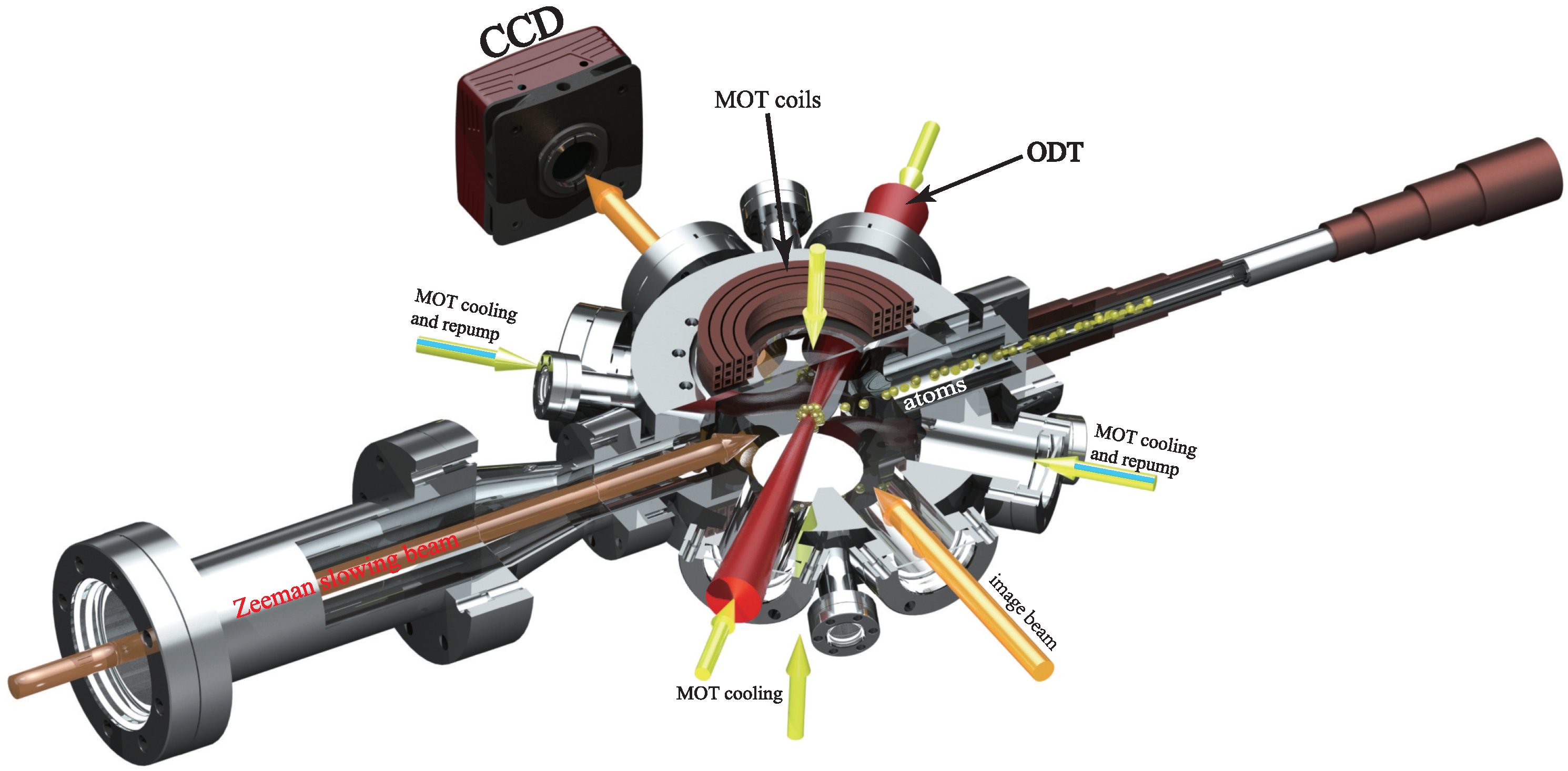
Figure 1.
Experimental apparatus of the science chamber and a part of the Zeeman slower. The science chamber is an octagonal chamber with 12 viewports. Magneto-optical trap (MOT) cooling beams (yellow arrows) and repump beams (blue line in yellow arrows) are coupled together. The Zeeman slowing beam (brown arrow) is used to decelerate the ejected atoms (yellow ball). A focused ODT (red arrow) along a cooling beam captures the atoms. The orange arrows represent the image beams.
The Zeeman slower [16] performs the first cooling step to slow down the atoms ejected from a pin hole in the oven chamber. A magneto-optical trap (MOT) [17] is used to further cool and collect the atoms. The MOT is constructed with six cooling beams in three orthogonal directions, two repump beams, and a pair of 12-turn anti-Helmholtz coils (Figure 1). The cooling and repump beams are provided by a frequency-doubled diode laser (TA-SHG pro, Toptica), of which the frequency is locked to the Na atomic transition line (). The MOT cooling beams are detuned by = −20 MHz from the cycling transition, have a power of 4.5 mW, and two of them combine with one 2.2 mW MOT repump beam. The magnetic field gradient is 10 G/cm. The frequency of MOT repump beams is nearly in resonance with the transition. After 8 s of MOT loading, we collect 6 × sodium atoms. Next, the atoms are transferred to a compressed MOT (CMOT) and an optical molasses [18] process efficiently cool 5 × atoms to 45 K (Figure 2). The atom gas is compressed by increasing the power of MOT cooling beams to 15 mW and reducing the power of MOT repump beams to 10 W as well as changing to −15 MHz in 3 ms. In this CMOT stage, we kept the magnetic field gradient unchanged to keep the atoms stable. The optical molasses performs 17 ms, in which the frequency of MOT cooling beams are detuned to = −30 MHz. Simultaneously, the power of the MOT cooling beams and the magnetic field gradient are linearly drops to 3.6 mW and 0.2 G/cm, respectively. The whole experimental sequence is shown in Figure 2. To de-pump atoms into the F = 1 hyperfine state, the repump beams are extinguished 1 ms before the MOT cooling beams, and the magnetic field gradient are turned off.
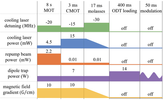
Figure 2.
Experimental sequence of parametric excitation of atoms in the ODT. The axes are not to scale.
The next step is to load the pre-cooled atoms into the ODT. An ODT captures the atoms by the interaction of the induced dipole moment with the intensity gradient of the light field. For a far-off-resonance-detuned laser, the scattering rate and the optical potential for atoms are given by [19]:
where c is the speed of light, ℏ is the reduced Planck constant, is the resonant transition frequency, is the detuning of the laser, is the natural decay rate of the excited state in radians per second, I is the intensity of the laser, and r is the spatial coordinate. Equations (1) and (2) show that a large-detuned and high-intensity dipole trap can maintain low scattering rates for a certain potential depth.
In the experiment, a fiber-amplified laser (1070 nm, IPG-FLR-LP) with a power of 100 W is used to provide a large-detuned and high-intensity dipole trap laser. A dipole trap laser is focused to the atoms and has a waist of 32 m. As shown in Figure 2, the power of the dipole trap laser is kept at half power (7 W) during the entire laser cooling process and is then jumped to the maximum (14 W). This process can effectively improve the ODT capture efficiency of atoms. [20] After a 400 ms ODT loading, the ODT captures about 1 × 10 atoms at a temperature of ∼80 K. The phase space density is ∼0.3 × 10. According to Equation (1) and the parameters of our ODT, we have calculated that the trap frequency is about 2.46 kHz.
Then we need to parametrically modulate the trapping potential that the atoms experience. An arbitrary function generator (Textronix AFG31153) is used to generate a modulation signal with an adjustable frequency, amplitude and waveform. The modulation signal and the analog signal are mixed by a summing amplifier (SRS SIM980). (The analog signal is used to control the power of the dipole trap laser. The power of the dipole trap laser can be modulated by the modulation signal.) The mixed signal is sent to a voltage-controlled oscillator (VCO) to generate a synthesized signal that can control the diffraction efficiency of the acousto-optic modulator (AOM). The synthesized signal is sent to the AOM through an amplifier to control and modulate the power of the first-order diffracted beam (the dipole trap laser). After the AOM, the diffracted beam is sent to the atoms through an optical fiber, which avoids the effects on the position change of the beam when the RF power of the AOM is modulated. Therefore, the trapping potential (the power of the dipole trap laser) can be modulated with an amplitude and a frequency . The modulation time T is set to 50 ms. Absorption imaging of the atoms for each experiment is performed after the dipole trap and the modulation were turned off.
Two trap frequencies in both radial and axial directions exist, and the trap frequency in the loosely confined axial direction is far less than the trap frequency in the closely confined radial direction. In our experiment, we predominantly consider the evolution of the atoms at the radial resonances.
The modulation induces the atoms to oscillations at the modulation frequency in the ODT. If the modulation frequency equals twice the axial or radial trap frequency, the parametric heating is most drastic and most atoms loss would happen. Regarding the lowest energetic atoms, the modulation energy is insufficient for them to escape from the trap, as it would happen for a harmonic potential. [21] Conversely, atoms with high energy are easily heated out of the trap. The number of lost atoms will increase as the modulation amplitude (modulation depth) increases.
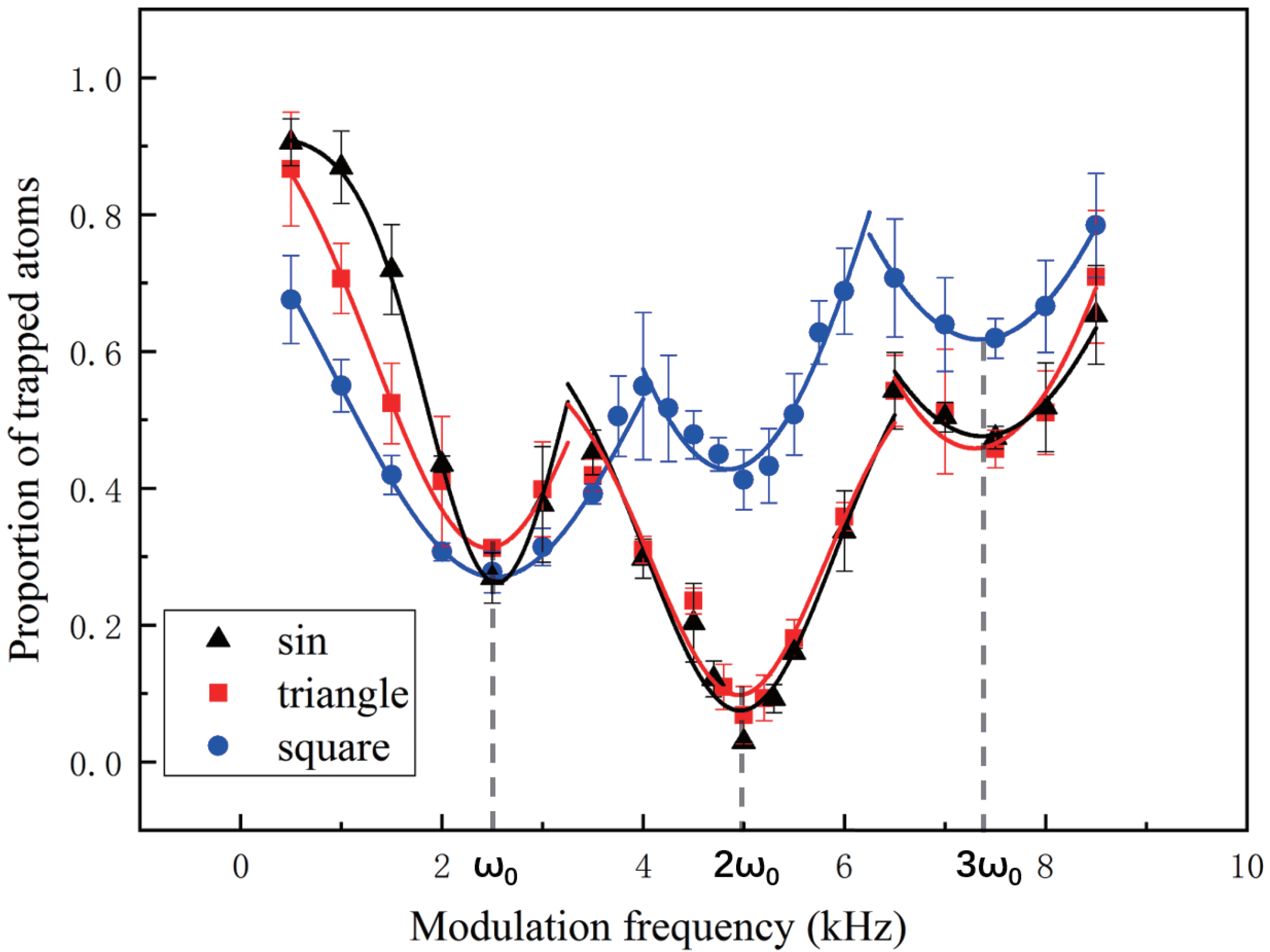
The relationship between the proportion of traped atoms and modulation frequency for three waveforms are shown in Figure 3. The range of the modulation frequency is set to 0.5–8.5 kHz, which covers 1 to 3 times the theoretical value (2.46 kHz), and each data point is measured three times. In order to avoid distortion of the modulated signal, we slightly reduce the power of the ODT. The initial number of atoms is about 6 × 10. We used the same modulation depth of 0.15 for the three wave forms to avoid the influence of the integral absolute intensities of the modulation signals. The modulation depth is the ratio of the effective amplitude to the total amplitude. In Figure 3, we can clearly see the three resonances loss at ∼2.47 (±0.19) kHz, ∼4.89 (±0.15) kHz and ∼7.31 (±0.27) kHz in the loss spectra. The three resonances loss match the frequency of , , and . By identifying three resonance frequencies and comparison with the theoretical value, the trap frequency (±0.19) kHz. The measured trap frequency is equal to the calculated value and should be accurate for the atoms at low levels of the harmonic potential. The trap frequency measurements for three type modulation is precise, and each modulation type can be used to measure the trap frequency.
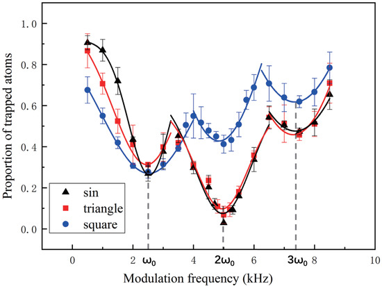
Figure 3.
The experimental spectrum of the losses associated to parametric excitation of the ODT modulated by a sine wave (black data), a triangle wave (red data) and a square wave (blue data). The modulation depth is 0.15. Gaussian fits were used to determine the resonance center position. The measured resonance positions are 2.47 (±0.19) kHz, ∼4.89 (±0.15) kHz and ∼7.31 (±0.27) kHz, corresponding to the frequencies of , , and , respectively.
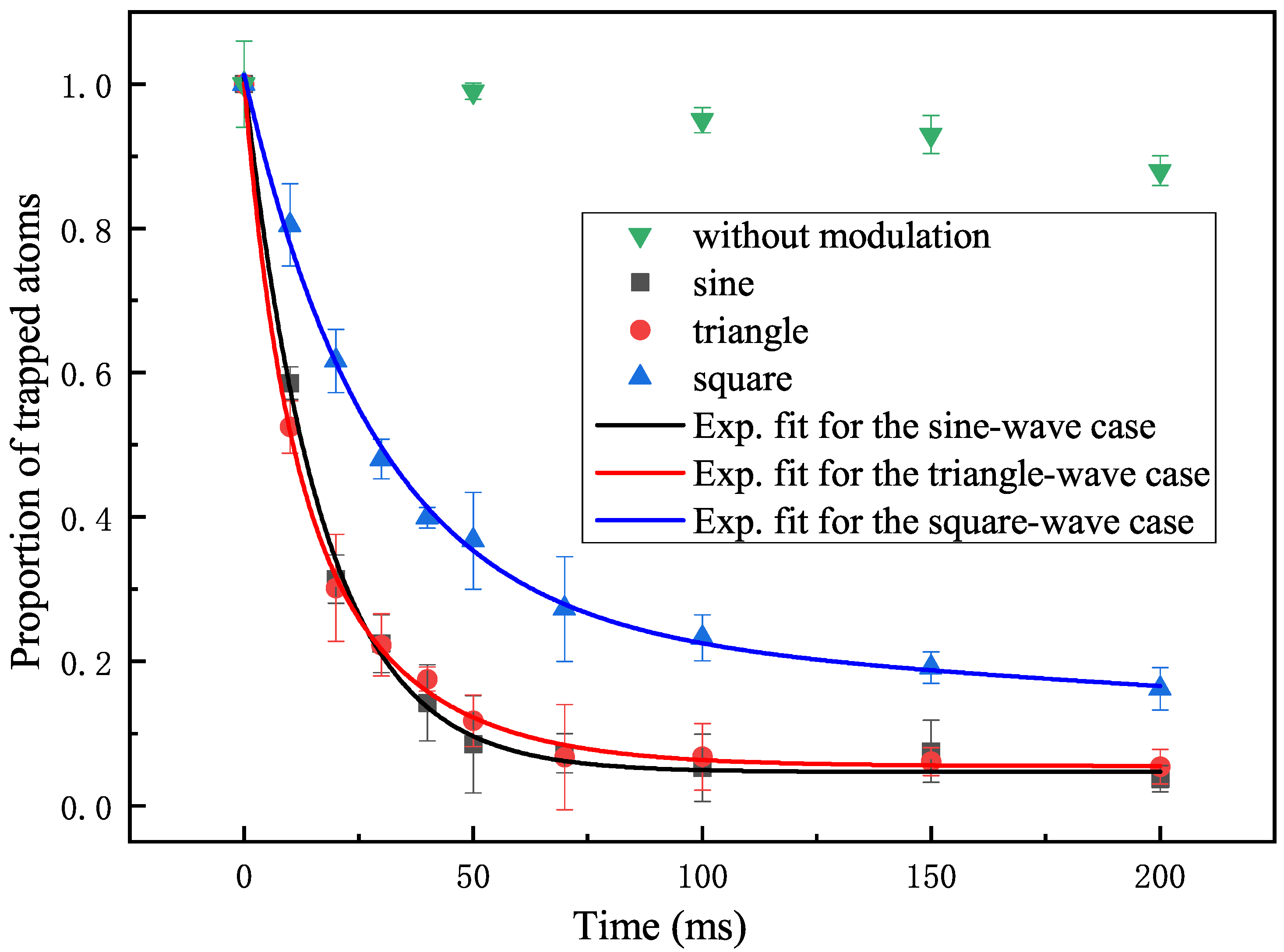
Figure 4 shows the results of the evolution of the trapped atoms population. As modulation time increases, the atom loss of sin and triangle wave modulation is faster than that of the square wave modulation. We also measured the lifetime of the atoms without modulation as 7.2 (±0.2) s (The data after 200 ms are not shown in the Figure 4). The comparison of the evolution of the trapped population with and without modulation shows that modulation can cause intense trap losses in a brief time.
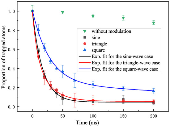
Figure 4.
Experimental result (data points) and theoretical fitting (colorful solid lines) of the evolution of the trapped atom population. The modulation frequencies are and the modulation depths are 0.15. The green points show an experimental trap loss measurement without modulation as a comparison.
3. Theoretical Simulation
To simulate the parametrically modulate optical potentials, in many previous works (e.g., [22] and references therein) the classical kinetic scheme with the transition probabilities computed in the first-order quantum mechanical perturbation theory for the model of the harmonic oscillator was employed. This approach implies a loss of the quantum coherence between transitions. However, the atomic ultracold ensembles are characterized by the long-living coherence. So, we apply a fully-coherent quantum mechanical calculation in the simulation.
The standard time-dependent Schrödinger equation is
where t is the time, is the Hamiltonian, is the time-dependent potential function, is the wavepacket of an atom in an ODT, is the momentum, x is the spatial coordinate, M is the mass, ℏ is the reduced Planck constant.
Assume that the potential function takes the form
where is a time–independent zero-th order potential, is a contribution to the overall perturbation, which could arise from a distortion of the shape of the potential well during the modulation and can also effectively comprise an effect of the time-independent perturbations, keeping the zeroth-order potential as simple as possible, and is some function of t (modulation signal). Then, is the spectrum of the zero-th order potential:
The quantities we are interested in are the time-dependent populations of the zero-th order states:
where
are the corresponding amplitudes. We assume that the number of atoms remained trapped by the instant t can be approximated by or, maybe, by a limited sum of few lowest .
In principle, the set of equations above can be solved directly.
Using Equation (3) with the substitution Equation (4), we can derive an equation for the amplitudes Equation (8)
Introducing the matrix notations
we can recast Equation (9) into the matrix form
with all the multiplications understood in the matrix sense. The text-book time dependent perturbation theory results in its solution:
where is the time-ordered exponent.
Hence, the first-order evolution operator in Equation (13) between the time instants and can be written as:
for which we only have to compute relatively simple integrals
while the quantities
are time-independent and can be computed beforehand from a precomputed spectrum of the time-independent Schrödinger equation (Equation (5)).
With a small enough time step , the evolution of the amplitude vector can be approximated by
Further on, we adopt the approximation of the harmonic oscillator:
where is the vibrational quantum number. In this case the matrix elements of W can be computed analytically.
In terms of the dimensionless coordinate,
where a and are the standard annihilation and creation operators, the recurrence relations
are valid, enabling a computation of the matrix elements for all k, n, m of interest starting with ( is the Kronecker symbol). We also assume that the term in the perturbation can be expressed as a power series in :
with measured in the units of the circular frequency . This way, all the quantities and (Equation (16)) as well as the entire matrix W (Equation (11)) are easily computed.
Let be a periodic function with the period so that . For the simplest modulation signals of our interest, the integrals (Equation (15)) can be computed analytically, e.g., for the sinusoidal signal in a pure harmonic approximation:
However, such expressions contain indeterminate forms at , requiring special treatment. In practical computations, it is easier to estimate the integrals (Equation (15)) directly with some numerical algorithm. For the small enough time step (, ) the simple approximation can be appropriate:
however, in our computations we used a more elaborate integration procedure (see below).
Besides the sinusoidal signal, we consider the square modulation signals:
and the triangular modulation signal
where is the modulo (remnant in division of t by T).
In the material above, we implied that a physical Hamiltonian is the Hermitian operator, resulting in the unitary evolution operator. In this case, the evolution remains conservative, so that no atoms escape the system, showing a kind of an oscillatory behavior of the individual levels’ populations. In order to simulate a possible escape from the ODT after every time step of the length (with Equation (17)), we first renormalized the vector (it is necessary as the first-order evolution operator is able to violate the norm conservation) and then multiplied the amplitudes by a damping factor with an adjustable parameter for all levels starting with (i.e., the lowest level retained untouched).
In agreement with our experimental parameters, we performed test computations: rad/s; ms; ms; (the pure harmonic approximation) and rad/s (the cubic perturbation); ; the computation included 11 () lowest levels of the harmonic potential well. The amplitude C is set to , and 0.15 for sin, triangle, and square wave modulations, respectively, to ensure the same effective amplitude. The time step was chosen ms, the integrals (Equation (15)) were estimated with the rectangular rule using a net of 50 nodes within every -interval.

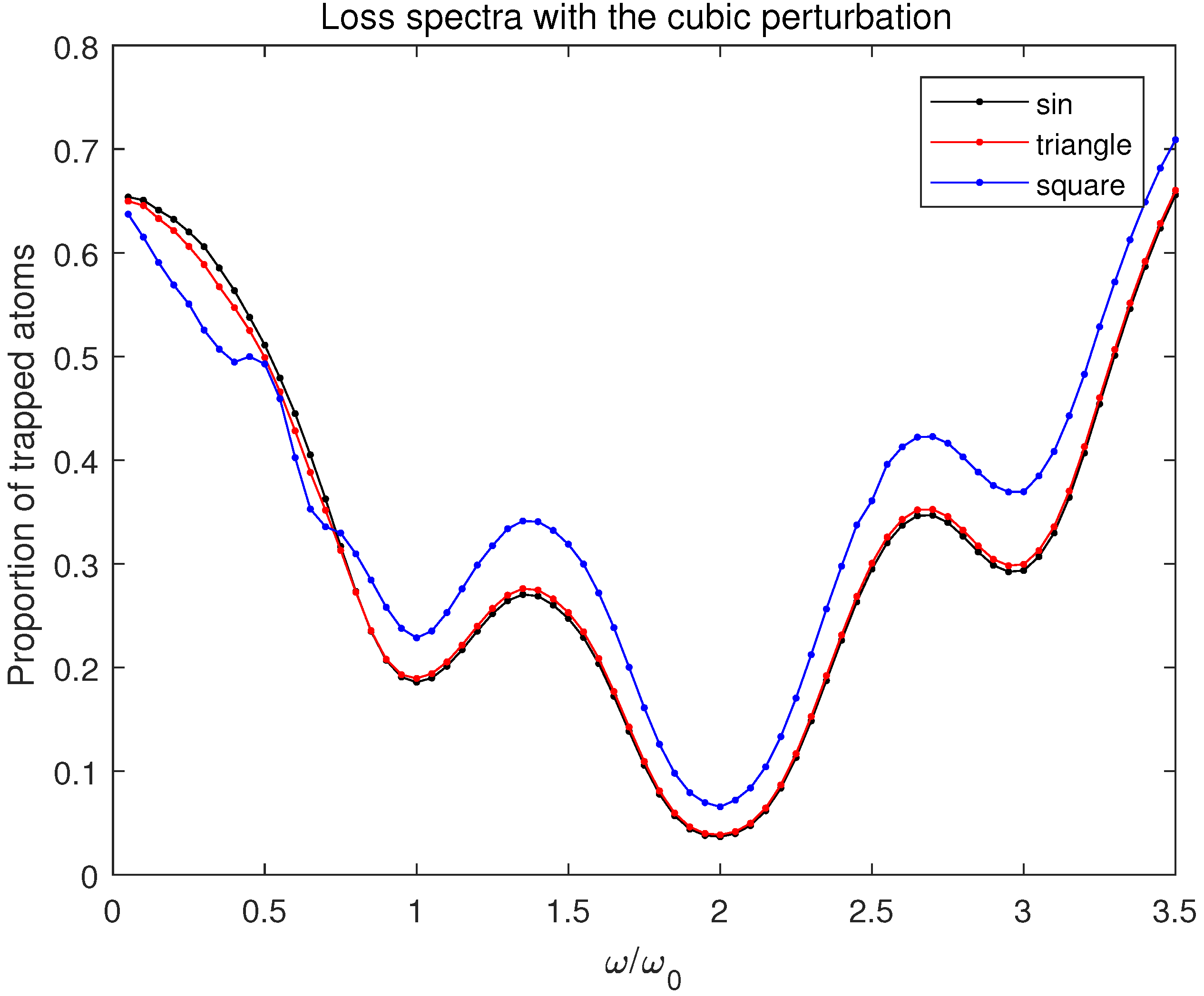
Figure 5.
Decimal logarithms of the simulated population of the lowest level vs. the relative frequency of the modulation signal at the instant ms, within the model described above: black—the sinusoidal modulation signal, red—the triangular modulation signal, blue—the square modulation signal.
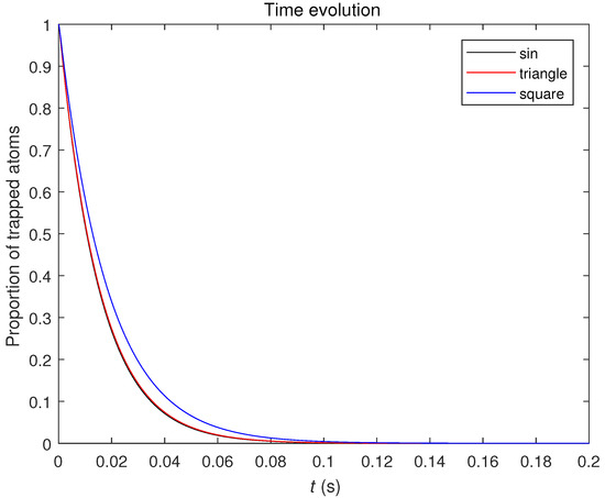
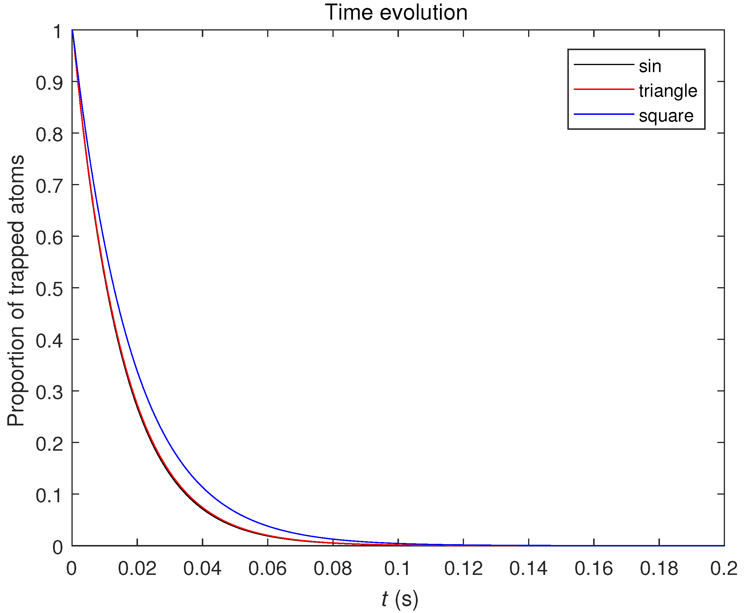
Figure 6.
Simulated time evolution of the lowest level population vs time (s) at the frequency of the modulation signal, within the model described above: black—the sinusoidal modulation signal, red—the triangular modulation signal, blue—the square modulation signal.
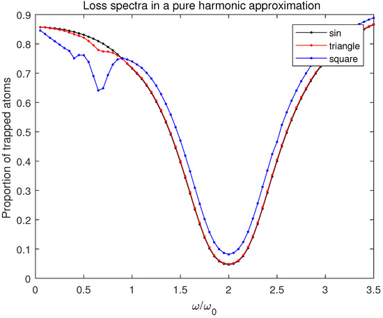
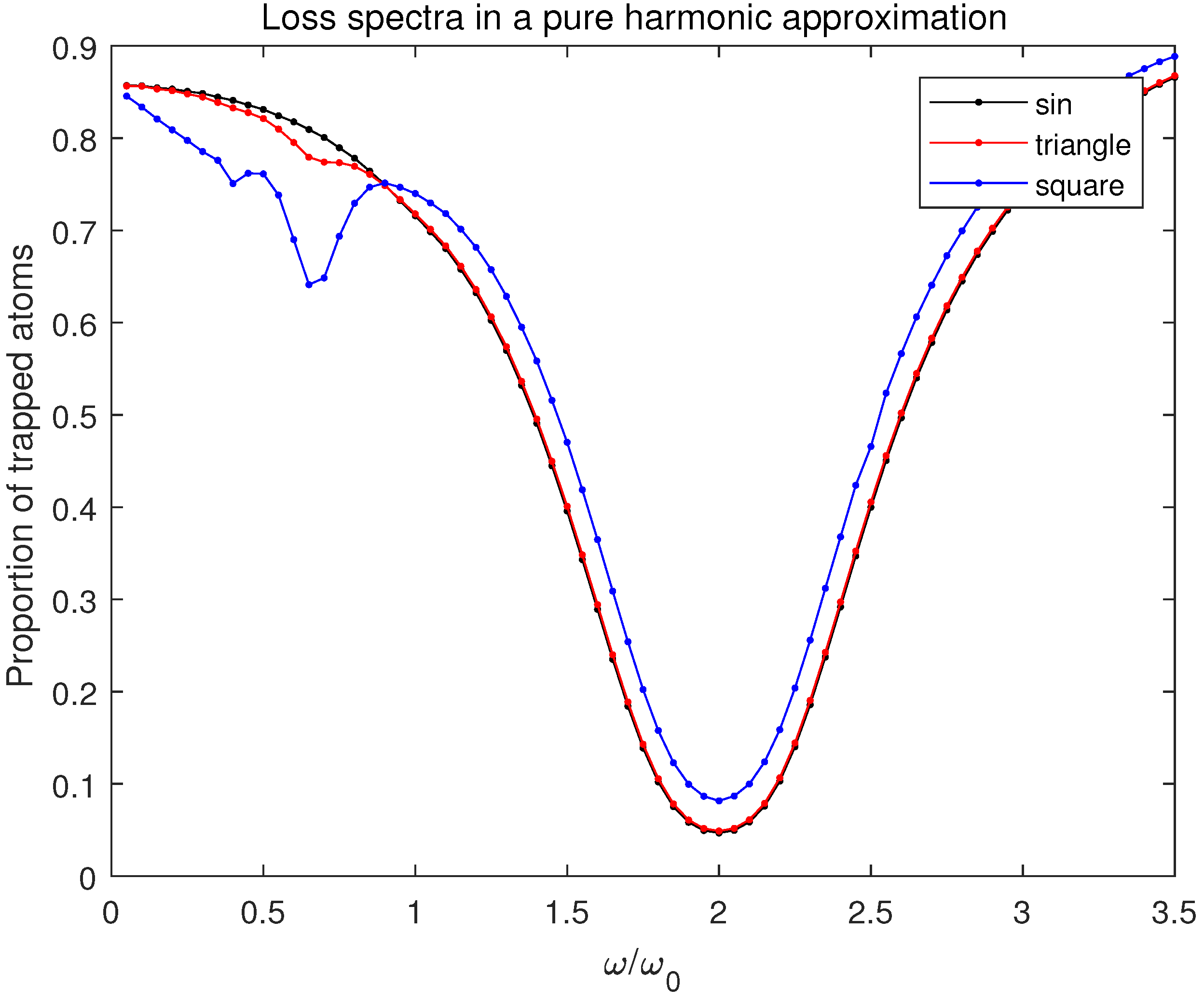
Figure 7.
Decimal logarithms of the simulated population of the lowest level vs the relative frequency of the modulation signal at the instant ms, within the pure harmonic (i.e., with ) model described above: black—the sinusoidal modulation signal, red—the triangular modulation signal, blue—the square modulation signal.
Figure 5 shows the loss spectra at the terminal time ms computed with the cubic perturbation (see Equations (4) and (22)). The classical theory of the parametrically driven harmonic oscillator [23] results in a conclusion that the resonance occurs at the modulation circular frequency of with being the principal circular frequency of the unperturbed harmonic oscillator. In our theoretical simulation, the majoring resonance at and two other strong resonances at and appeared. Their origin is the transitions with (m and n are vibrational quantum numbers) and , allowed for in this more elaborate model. The extra resonances at () [24], clearly seen in Figure 7, contribute noticeably to the square-wave case as well. The forms of the resonances in Figure 5 resemble the ones observed experimentally, in spite of the relative simplicity of our computational model.
Figure 6 shows the time evolution of the lowest level populations for the three modulation signals, computed within our model. The harmonic potential is completely bound, so the excited atoms would not leave its range. The real ODT potential is unbound; hence, the part of atoms with high enough energy would escape as soon as their energy reaches the ODT potential limit. We expect that this process goes on exponentially, [25] resulting in an approximately exponential time dependence of the observed atomic losses. The experimental results (Figure 4) under different waveforms correlate well with the theoretical analysis. As expected, they exhibit exponential-like behavior in Figure 6. We consider the evolution of the population of atoms in the trap under different types of ODT modulation.
Figure 7 shows the loss spectra at the terminal time ms computed within the pure harmonic approximation () for the three types of the modulation signal. All the spectra exhibit one strong resonance at the frequency of the modulation signal , reflecting the fact that transitions between the levels separated by with the uniform energy intervals are only possible. The case of the square wave (and of the triangle one but much weaker) also exhibits extra resonances at the frequencies with the odd integer . These extra resonances occur due to the fact that the square- and triangular-wave signals with the frequencies contain noticeable harmonics of the majoring resonance frequency ; the ones with even integer k do not contribute because the corresponding integrals Equation (15) over the full period are zero for the kind of signals considered here.
In order to substantiate our approach, we estimated the average time between collisions of the gas kinetic theory as , with our measured values of the atomic spatial density and the mean velocity v, while for the radius R of the sodium atom we took a standard table value of 200 pm. The estimated time was close to 1 s, which is several orders of magnitude longer than the time scale of our experiments. This means that most atoms in the ODT do not experience collisions during the experiment and behave as independent quantum particles in the ODT potential. This justifies our pure quantum-mechanical treatment. On the other hand, we deal with a quite simple model of the ODT potential, so that both our quantum-mechanical and the kinetic approaches remain no more than phenomenological and are appropriate as long as they are able to explain the physics behind the observations. The theoretical model considered the three simple modulation types that can be easily extended to some complex waveform modulation.
4. Discussion
For the modulation of sine and triangle waves in Figure 3, the experimental results show a good accordance with the theoretical simulation and the maximum atom loss occurs at . However, for the square wave modulation in Figure 3, the maximum atom loss occurs at , which is inconsistent with our theoretical model. Considering the high-order harmonics of the square wave, the resonances loss near and are predicted to exist in the theoretical model (Figure 5) but not observed in Figure 3. Their superpositions possibly caused the loss at to be deeper and wider than predicted. Apart from that, the experimental results show a good accordance with the theoretical simulation for the square wave modulation.
For a continuous waveform modulation, the theoretical model shows good experimental reproducibility. However, for a discontinuous waveform modulation, the theoretical model shows some defects. One of the reasons for the more noticeable disagreement of the modeled and experimental spectra in the case of the square-wave modulation can be the use of the first-order perturbation theory. Indeed, this approach presumes that the signal changes slowly within the time step of the computational scheme. Meanwhile, the square-wave signal exhibits abrupt discontinuities. Nevertheless, even for this signal, our approach showed clear resonances at expected frequencies. Experimentally, another reason for the discrepancy in the experiment of square wave modulation is the distortion of the signals caused by the response time of the AOM.
5. Conclusions
We have investigated both experimentally and theoretically the resonance loss spectra and the time evolution of the trapped atom populations in an ODT by a parametric excitation using the multi-waveform modulation. The trap frequency is systematically measured under three common waveform modulations (sine, triangle, and square waves). We presented a heuristic model for the excitation in a harmonic trapping potential under various waveforms. Although the model does not provide a sufficient explanation of the real physical situation, the theoretical simulations correlate well with the principal features of both the spectra of trap losses, including the appearance of resonances, and the time evolution of the total number of trapped atoms. The theoretical analysis can be easily extended to complex waveform modulation and reproduces enough of the experiments. Parametric modulation is also an effective method for studying atomic dynamics. The dynamical analysis can be easily extended to a higher dimensional optical trap or lattice. The modulation of different waveforms can lay the foundation for a more detailed understanding of the shape of the potential trap and dynamic analysis of atoms in a trap in the future.
Author Contributions
N.Z. and W.L. peformed the experiments. J.W. and J.M. supervised the experimental work. Y.L. interpreted data and critical reading of the manuscript. V.S. contributed the theoretical analysis. All authors contributed to the analysis and discussions of the results and the preparation of the manuscript. All authors have read and agreed to the published version of the manuscript.
Funding
This work is supported by the National Key R&D Program of China (Grant No. 2017YFA 0304203), the National Natural Science Foundation of China (Grants Nos. 62020106014, 62175140, 92165106, 12104276, 62011530047), PCSIRT (No. IRT-17R70), 111 project (Grant No. D18001), the Applied Basic Research Project of Shanxi Province, China (Grant No. 201901D211191, 201901D211188), the Shanxi 1331 KSC.
Institutional Review Board Statement
Not applicable.
Informed Consent Statement
Not applicable.
Data Availability Statement
Data underlying the results presented in this paper are not publicly available at this time but may be obtained from the authors upon reasonable request.
Conflicts of Interest
The authors declare no conflict of interest.
References
- Adams, C.S.; Lee, H.J.; Davidson, N.; Kasevich, M.; Chu, S. Evaporative cooling in a crossed dipole trap. Phys. Rev. Lett. 1995, 74, 3577. [Google Scholar] [CrossRef] [PubMed]
- Büchler, H.P.; Demler, E.; Lukin, M.; Micheli, A.; Prokof’Ev, N.; Pupillo, G.; Zoller, P. Strongly correlated 2D quantum phases with cold polar molecules: Controlling the shape of the interaction potential. Phys. Rev. Lett. 2007, 98, 060404. [Google Scholar] [CrossRef] [PubMed] [Green Version]
- Bloch, I.; Dalibard, J.; Nascimbene, S. Quantum simulations with ultracold quantum gases. Nat. Phys. 2012, 8, 267–276. [Google Scholar] [CrossRef]
- Barredo, D.; Labuhn, H.; Ravets, S.; Lahaye, T.; Browaeys, A.; Adams, C.S. Coherent excitation transfer in a spin chain of three Rydberg atoms. Phys. Rev. Lett. 2015, 114, 113002. [Google Scholar] [CrossRef] [PubMed] [Green Version]
- De Paz, A.; Sharma, A.; Chotia, A.; Marechal, E.; Huckans, J.; Pedri, P.; Santos, L.; Gorceix, O.; Vernac, L.; Laburthe-Tolra, B. Nonequilibrium quantum magnetism in a dipolar lattice gas. Phys. Rev. Lett. 2013, 111, 185305. [Google Scholar] [CrossRef] [PubMed]
- Balik, S.; Win, A.; Havey, M. Imaging-based parametric resonance in an optical dipole-atom trap. Phys. Rev. A 2009, 80, 023404. [Google Scholar] [CrossRef] [Green Version]
- Strogatz, S.H. Nonlinear Dynamics and Chaos: Lab Demonstrations; Internet-First University Press: Boca Raton, FL, USA, 1994. [Google Scholar]
- Collet, P.; Courbage, M.; Métens, S.; Neishtadt, A.; Zaslavsky, G. Chaotic Dynamics and Transport in Classical and Quantum Systems, Proceedings of the NATO Advanced Study Institute on International Summer School on Chaotic Dynamics and Transport in Classical and Quantum Systems, Cargèse, Corsica, 18–30 August 2003; Springer Science & Business Media: Dordrecht, The Netherlands, 2006; Volume 182. [Google Scholar]
- Boulier, T.; Maslek, J.; Bukov, M.; Bracamontes, C.; Magnan, E.; Lellouch, S.; Demler, E.; Goldman, N.; Porto, J. Parametric heating in a 2D periodically driven bosonic system: Beyond the weakly interacting regime. Phys. Rev. X 2019, 9, 011047. [Google Scholar] [CrossRef] [Green Version]
- Arnal, M.; Brunaud, V.; Chatelain, G.; Cabrera-Gutiérrez, C.; Michon, E.; Cheiney, P.; Billy, J.; Guéry-Odelin, D. Evidence for cooling in an optical lattice by amplitude modulation. Phys. Rev. A 2019, 100, 013416. [Google Scholar] [CrossRef] [Green Version]
- Hudomal, A.; Regnault, N.; Vasić, I. Bosonic fractional quantum Hall states in driven optical lattices. Phys. Rev. A 2019, 100, 053624. [Google Scholar] [CrossRef] [Green Version]
- Li, J.; Liu, J.; Xu, W.; de Melo, L.; Luo, L. Parametric cooling of a degenerate Fermi gas in an optical trap. Phys. Rev. A 2016, 93, 041401. [Google Scholar] [CrossRef] [Green Version]
- Ferris, A.J.; Davis, M.J.; Geursen, R.W.; Blakie, P.B.; Wilson, A.C. Dynamical instabilities of Bose-Einstein condensates at the band edge in one-dimensional optical lattices. Phys. Rev. A 2008, 77, 012712. [Google Scholar] [CrossRef] [Green Version]
- Kumakura, M.; Shirahata, Y.; Takasu, Y.; Takahashi, Y.; Yabuzaki, T. Shaking-induced cooling of cold atoms in a magnetic trap. Phys. Rev. A 2003, 68, 021401. [Google Scholar] [CrossRef]
- Poli, N.; Brecha, R.J.; Roati, G.; Modugno, G. Cooling atoms in an optical trap by selective parametric excitation. Phys. Rev. A 2002, 65, 021401. [Google Scholar] [CrossRef] [Green Version]
- Bell, S.; Junker, M.; Jasperse, M.; Turner, L.; Lin, Y.J.; Spielman, I.; Scholten, R.E. A slow atom source using a collimated effusive oven and a single-layer variable pitch coil Zeeman slower. Rev. Sci. Instrum. 2010, 81, 013105. [Google Scholar] [CrossRef]
- Marcassa, L.; Bagnato, V.; Wang, Y.J.; Tsao, C.; Weiner, J.; Dulieu, O.; Band, Y.; Julienne, P.S. Collisional loss rate in a magneto-optical trap for sodium atoms: Light-intensity dependence. Phys. Rev. A 1993, 47, R4563. [Google Scholar] [CrossRef]
- Chu, S.; Hollberg, L.; Bjorkholm, J.E.; Cable, A.; Ashkin, A. Three-dimensional viscous confinement and cooling of atoms by resonance radiation pressure. Phys. Rev. Lett. 1985, 55, 48. [Google Scholar] [CrossRef] [Green Version]
- Grimm, R.; Weidemüller, M.; Ovchinnikov, Y.B. Optical dipole traps for neutral atoms. Adv. At. Mol. Opt. Phys. 2000, 42, 95–170. [Google Scholar]
- Jiang, J.; Zhao, L.; Webb, M.; Jiang, N.; Yang, H.; Liu, Y. Simple and efficient all-optical production of spinor condensates. Phys. Rev. A 2013, 88, 033620. [Google Scholar] [CrossRef] [Green Version]
- Friebel, S.; D’Andrea, C.; Walz, J.; Weitz, M.; Hänsch, T. CO 2-laser optical lattice with cold rubidium atoms. Phys. Rev. A 1998, 57, R20. [Google Scholar] [CrossRef]
- Jáuregui, R.; Poli, N.; Roati, G.; Modugno, G. Anharmonic parametric excitation in optical lattices. Phys. Rev. A 2001, 64, 033403. [Google Scholar] [CrossRef] [Green Version]
- Landau, L.; Lifshitz, E. Mechanics. In Course of Theoretical Physics; Elsevier: Amsterdam, The Netherlands, 1976; Chapter 5; Volume 1, p. 58. [Google Scholar]
- Landau, L.; Lifschitz, E. Kleine Schwingungen. In Mechanik; Springer: Braunschweig, Germany, 1962; pp. 70–116. [Google Scholar]
- Savard, T.; O’hara, K.; Thomas, J. Laser-noise-induced heating in far-off resonance optical traps. Phys. Rev. A 1997, 56, R1095. [Google Scholar] [CrossRef] [Green Version]

Publisher’s Note: MDPI stays neutral with regard to jurisdictional claims in published maps and institutional affiliations. |
© 2022 by the authors. Licensee MDPI, Basel, Switzerland. This article is an open access article distributed under the terms and conditions of the Creative Commons Attribution (CC BY) license (https://creativecommons.org/licenses/by/4.0/).