Sensing by Dynamics of Lasers with External Optical Feedback: A Review

Abstract

External optical feedback (EOF) has great impacts on the properties of lasers. It influences the stable operation of lasers. However, various applications based on lasers with EOF have been developed. One typical example is self-mixing interferometry technology, where modulated steady-state laser intensity is utilized for sensing and measurement. Other works show that laser dynamics can also be used for sensing, and the laser in this case is more sensitive to EOF. This paper reviews the sensing technology that uses the dynamics of lasers with EOF. We firstly introduce the basic operating principles of a laser with EOF and discuss the noise properties of and intensity modification in lasers induced by EOF. Then, sensing applications using laser dynamics are categorized and presented, including sensing by frequency-shifted optical feedback, relaxation oscillation frequency, and dynamics with self-mixing interferometry signals and laser optical chaos. Lastly, we present an analysis of the transient response waveform and spectrum of a laser with EOF, showing its potential for sensing.

1. Introduction

External optical feedback (EOF) influences the properties and behavior of a laser [1]. Such optical feedback has been considered as a serious problem that degrades the performance of lasers [2,3]. However, various applications based on lasers with EOF have been developed. Typical examples are self-mixing interferometry (SMI) or optical feedback interferometry (OFI), which are emerging and promising non-contact sensing techniques using the self-mixing effect that occur when a fraction of light is back-reflected or back-scattered by an external target and re-enters the laser’s inside cavity [4,5,6,7,8,9]. In this case, the steady-state intensity of the lasing light is modulated by a varying external optical feedback phase, which is a remarkably universal phenomenon occurring in lasers regardless of type. The basic structure of a typical SMI system is depicted in Figure 1, which consists of a laser diode (LD), an integrated photodiode (PD) in the LD package, a lens, and an external target to be measured. This configuration reflects a minimum part-count scheme, which is useful for engineering implementation. SMI-based sensing and detection have been developed for different applications such as the measurement of displacement [10,11], distance [12,13,14], speed [15,16], mechanical parameters of materials [17,18], laser parameters [19,20], angle [21,22], acoustic field [23,24,25], biomedical signals [26,27,28], the characterization of micro-machined silicon gyroscopes [29], and monitoring plasma accumulation in laser ablation [30,31].

For all the above applications, the laser operates in a steady state and the modulated steady-state laser intensity is used as the sensing signals, also called SMI signals. Recently, sensing and measurement by using laser dynamics have been reported and higher sensitivity compared with the conventional SMI has also been demonstrated [32]. The progress of SMI technology was reviewed in several works [33,34,35,36,37,38] but few have focused on a review of sensing by the dynamics of lasers with EOF.

This work aims to provide an overview of sensing by the dynamics of lasers with EOF. The rest of the paper is organized as follows. Section 2 reveals the basic operating principle of lasers with EOF and presents discussion on the noise properties and intensity modification in lasers induced by EOF. Section 3 presents categorized sensing applications using the dynamics of lasers with EOF, including sensing by frequency-shifted optical feedback, relaxation oscillation frequency, dynamics in SMI signals and laser chaos. Then, a method to investigate the transient response waveform and spectrum of lasers with EOF is also proposed in this section, showing the potential of using them for sensing. Finally, a summary is included in Section 4.

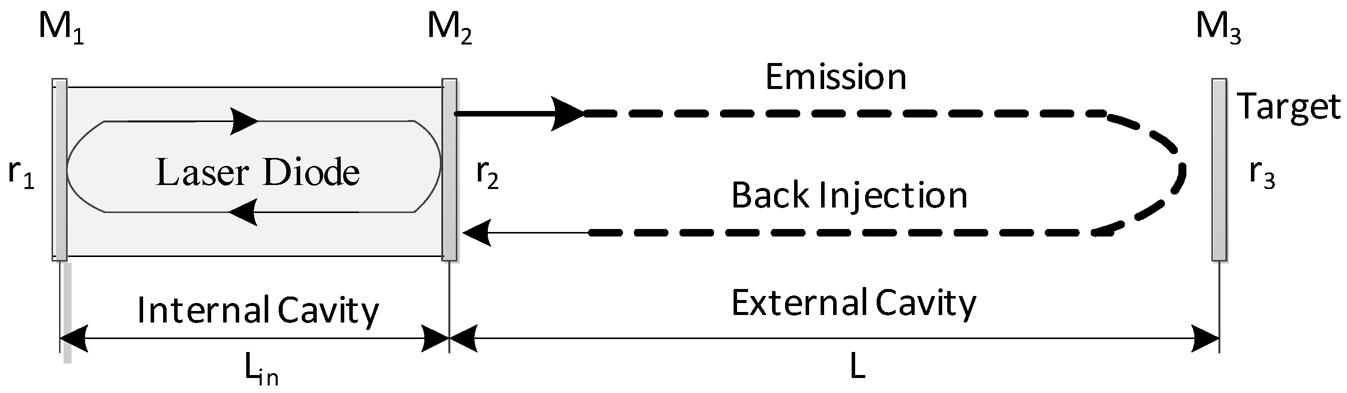
2. Operating Principle

In 1980, Lang and Kobayashi analyzed EOF effects on LD properties and proposed the standard Lang–Kobayashi (L–K) equation to describe its behavior by adding a component representing the EOF effects to the rate equations of an LD, as follows [1]:

$$\frac{d\widehat{\mathit{E}(\mathit{t})}}{dt}=\left\{\frac{1+i\alpha }{2}\left[G[N(t),\widehat{\mathit{E}(\mathit{t})}]-\frac{1}{{\tau }_p}\right]+i{\omega }_0\right\}\widehat{\mathit{E}(\mathit{t})}+\frac{\kappa }{{\tau }_{in}}\cdot \widehat{\mathit{E}(\mathit{t}-\mathit{\tau })}.$$

(1)

Equation (1) can be explained with Figure 2, where the facet amplitude reflectivity of back facet M1 and front facet M2 is denoted by r₁ and r₂, respectively. The external target has an amplitude reflectivity, r₃. Some of the emission light is back-reflected by the target and re-injects to the laser’s internal cavity. Considering the weak to moderate optical feedback levels, only one reflection in the external cavity is included. Hence, in Equation (1), the last term accounts for the back-reflection from the target, i.e., the EOF, and the other terms are for the solitary laser diode without EOF. The optical feedback strength is evaluated by the parameter κ, which is expressed as $\kappa =\sigma r_3(1-r_2{}^2)/r_2$, where σ ≤ 1 represents the possible loss on the back injection, i.e., mode mismatch.

In Equation (1), $\widehat{\mathit{E}(\mathit{t})}$ is the complex photoelectric field which contains slow varying complex filed $\mathit{E}(\mathit{t})$ and fast optical angular frequency ${\omega }_0$. The variation of electric-field amplitude is much slower than the optical angular frequency ${\omega }_0$. So, the fast optical oscillation component can be separated from the slow complex electric field $\mathit{E}(\mathit{t})$ as below:

$$\widehat{\mathit{E}(\mathit{t})}=\mathit{E}(\mathit{t})e^{i{\omega }_{0}t}.$$

(2)

Substituting Equation (2) into Equation (1), we can obtain:

$$\begin{array}{l}\frac{d\mathit{E}(\mathit{t})}{dt}=\frac{1+i\alpha }{2}\left\{G[N(t),\widehat{\mathit{E}(\mathit{t})}]-\frac{1}{{\tau }_p}\right\}\mathit{E}(\mathit{t})+\frac{\kappa }{{\tau }_{in}}\cdot e^{-i{\omega }_0\tau }\mathit{E}(\mathit{t}-\mathit{\tau }). \\ \end{array}$$

(3)

The slow complex electric field $\mathit{E}(\mathit{t})$ can be written by the real values of the amplitude $\mathit{E}(\mathit{t})$ and phase $\varphi (t)$ as follows:

$$\mathit{E}(\mathit{t})=\mathit{E}(\mathit{t})e^{i\varphi (t)}.$$

(4)

In laser theory, photon density, denoted by S(t), is usually used to describe the laser mechanism when considering the effect of spontaneous emission and statistical Langevin noises, which is expressed as [39]:

$$S(t)={\left|\mathit{E}(\mathit{t})\right|}^2=\mathit{E}(\mathit{t}){\mathit{E}}^{*}(\mathit{t}).$$

(5)

From Equations (4) and (5), we can obtain:

$$\frac{dS(t)}{dt}=2\mathrm{Re}[{\mathit{E}}^{*}(\mathit{t})\frac{d\mathit{E}(\mathit{t})}{dt}],$$

(6)

$$\frac{d\varphi (t)}{dt}=\frac{1}{S(t)}\mathrm{Im}[{\mathit{E}}^{*}(\mathit{t})\frac{d\mathit{E}(\mathit{t})}{dt}].$$

(7)

Substituting Equations (3) and (4) into Equations (6) and (7), and adding the terms accounting for spontaneous emission and statistical Langevin noises [40,41], we obtain:

$$\frac{dS(t)}{dt}=\left\{G[N(t),\widehat{\mathit{E}(\mathit{t})}]-\frac{1}{{\tau }_p}\right\}\mathit{E}(\mathit{t})+2\frac{\kappa }{{\tau }_{in}}\sqrt{S(t)S(t-\tau )}\cdot \cos \left[{\omega }_0\tau +\varphi (t)-\varphi (t-\tau )\right]+R_{sp}+F_S(t),$$

(8)

$$\frac{d\varphi (t)}{dt}=\frac{1}{2}\alpha \left\{G[N(t),\widehat{\mathit{E}(\mathit{t})}]-\frac{1}{{\tau }_p}\right\}-\frac{\kappa }{{\tau }_{in}}\sqrt{\frac{S(t-\tau )}{S(t)}}\sin \left[{\omega }_0\tau +\varphi (t)-\varphi (t-\tau )\right]+F_{\varphi }(t).$$

(9)

Another variable of describing lasers with optical feedback is carrier density $N(t)$, which is coupled with Equations (8) and (9) through the gain term of $G\left[N(t),\widehat{\mathit{E}(\mathit{t})}\right]=G_N\left[N(t)-N_0\right]\left[1-\epsilon \Gamma {\mathit{E}}^2(\mathit{t})\right]=G_N\left[N(t)-N_0\right]\left[1-\epsilon \Gamma S(t)\right]$. $N(t)$ is expressed as follows:

$$\frac{dN(t)}{dt}=\frac{J}{ev}-\frac{N(t)}{{\tau }_s}-G[N(t),\widehat{\mathit{E}(\mathit{t})}]{\mathit{E}}^2(\mathit{t})+F_N(t).$$

(10)

Equations (8)–(10) consist of the normal L-K equations, where R_sp accounts for spontaneous emission, $F_S(\mathrm{t})$, and $F_N(\mathrm{t})$ are Langevin noise forces, which are given by [41]:

$$R_{sp}=\frac{\gamma N(t)\Gamma }{{\tau }_s},$$

(11)

$$F_S(t)=\sqrt{\frac{2S(t)}{\Delta t}{R}_{sp}}{\chi }_S,$$

(12)

$$F_{\varphi }(t)=\sqrt{\frac{2}{S(t)\Delta t}{R}_{sp}}{\chi }_{\varphi },$$

(13)

$$F_N(t)=\sqrt{\frac{2N(t)}{{\tau }_s\Delta t}}{\chi }_N-\sqrt{\frac{2S(t)}{\Delta t}{R}_{sp}}{\chi }_S.$$

(14)

where ${\chi }_S$, ${\chi }_{\varphi }$, and ${\chi }_N$ denote Gaussian random variables with zero mean and unity standard deviation, and $\Delta t$ is the time interval over which the noise is held constant in the numerical model. The physical meanings and typical values of the laser-related parameters in Equations (8)–(14) are presented in

Table 1. Physical meanings and typical values of the symbols in the L–K equations.

	Symbol	Physical Meaning	Value
Fixed Parameters	$G_N$	modal gain coefficient	$8.1\times {10}^{-13} {\mathrm{m}}^3{\mathrm{s}}^{-1}$
	$N_0$	carrier density at transparency	$1.1\times {10}^{24} {\mathrm{m}}^{-3}$
	$\epsilon$	nonlinear gain compression coefficient	$2.5\times {10}^{-23} {\mathrm{m}}^3$
	$\Gamma$	confinement factor	$0.3$
	${\tau }_p$	photon life time	$2.0\times {10}^{-12} \mathrm{s}$
	${\tau }_s$	carrier life time	$2.0\times {10}^{-9} \mathrm{s}$
	${\tau }_{in}$	internal cavity round-trip time	$8.0\times {10}^{-12} \mathrm{s}$
	$\alpha$	linewidth enhancement factor	$6.0$
	$\gamma$	spontaneous emission factor	${10}^{-5}$
	$r_1=r_2$	amplitude reflectivity	$0.55$
	$\sigma$	reinjection loss	$0.5$
	e	elementary charge	$1.6\times {10}^{-19} \mathrm{C}$
	V	volume of the active region	$1.0\times {10}^{-16}{ \mathrm{m}}^3$
Controllable Parameters	$r_3$	amplitude reflectivity of the external target
	$\kappa$	$\mathrm{optical} \mathrm{feedback} \mathrm{strength} \mathrm{with} \kappa =\sigma r_3(1-r_2{}^2)/r_2$
	$J$	injection current
	$L$	external cavity length
	$\tau$	$\mathrm{light} \mathrm{roundtrip} \mathrm{time} \mathrm{in} \mathrm{the} \mathrm{external} \mathrm{cavity} \mathrm{with} \tau =2L/c$

[41,42]. Note that, although the L–K equation is primarily for semiconductor lasers, it is also to be used for describing other types of lasers, e.g., solid-state lasers [32,43,44].

The dynamic behavior of lasers with EOF is governed by the injection current ($J$) to the laser and the parameters associated with the external cavity including optical feedback strength ($\kappa$), the amplitude reflectivity of the external target surface ($r_3$), and the light roundtrip time in the external cavity ($\tau$). The other parameters in the L–K equations are related to the solitary laser itself, and can be treated as constants for a certain laser, as shown in Table 1. With different operation parameters, i.e., $J$, $r_3$, L, and $\tau$, the laser with EOF exhibits abundant high-level dynamics, e.g., period-one oscillation, quasi-periodic oscillation, and chaos. Figure 3 shows a typical example of different dynamics by numerically solving the L-K equations, where (a) is steady state, (b) is period-one oscillation, (c) is quasiperiodic oscillation, and (d) is chaos. Note that, since the laser power P is with $P\propto S(t)={\left|\mathit{E}(\mathit{t})\right|}^2$, we take $S(t)={\left|\mathit{E}(\mathit{t})\right|}^2$ as the intensity as performed in the literature [36,40,45]. Since its first discovery, the dynamics of the laser with EOF have been intensively investigated and its potential sensing applications have been developed.

In practical applications, the noise characteristics of lasers is a significant parameter. The noise properties are also influenced by EOF. Relative intensity noise (RIN) is often used to characterize the laser intensity noise [40,46,47,48], which is expressed as [41]:

$$RIN=\frac{\overline{{[S(t)-\overline{S(t)}]}^2}}{{\overline{S(t)}}^2},$$

(15)

where $\overline{S(t)}$ is the mean photon density. RINs under different operation conditons can be obtained after numerially solving the L–K equations. In the simualtions, $\Delta t$ was taken with 10 ps as in [40,41] and thus the spectral range is 0–50 GHz. Figure 4 shows the typical results of RINs with different external reflectivity in which we can find the RIN is as low as −158 dB/Hz and is almost constant when the amplitude reflectivity r₃ is less than $4\times {10}^{-3}$. With the increase in r₃, RIN increases due to the relaxation oscillation becoming undamped, but it is still less than −140 dB/Hz and can satisfy the requirements for most laser applications. Note that Jth is the threshold injection current of the laser with the expression $J_{\mathrm{th}}=(N_0+1/G_N{\tau }_p)/{\tau }_s$ [49].

The influence of EOF on the laser output power was then invesigated. We solved the stationary solutions to Equations (8)–(10) by setting $dS(t)/d(t)=0$, $d\varphi (t)/d(t)={\omega }_{\mathrm{s}}-{\omega }_0$ and $dN(t)/d(t)=0$. Then, we obtained:

$$N_F=N_0+\frac{1}{G_N{\tau }_p}-\frac{2\kappa \cos ({\omega }_F\tau )}{{\tau }_{in}{G}_N},$$

(16)

$$S_F=\frac{(J/eV-N_F/{\tau }_s)}{G_N(N_F-N_0)},$$

(17)

where ω_F is the laser angular frequency with EOF, $N_F$ and $S_F$ are respectively the carrier density and photon density with EOF in the steady state. Inserting Equation (16) into Equation (17), with the condition of weak feedback $\kappa <0.01$ [50], we can obtain:

$$S_F=\frac{{\tau }_p}{{\tau }_s}*[\frac{J{\tau }_s}{eV}-(N_0+1\frac{1}{G_N{\tau }_P})+\frac{2\kappa \cos ({\omega }_F\tau )}{{\tau }_{in}{G}_N}]*[1+\frac{2\kappa {\tau }_p\cos ({\omega }_F\tau )}{{\tau }_{in}}].$$

(18)

With the similar treatment and setting $\kappa =0$, we obtain the laser output intensity in the steady state without EOF as below:

$$S_{NF}=\frac{{\tau }_p}{{\tau }_s}[\frac{J{\tau }_s}{eV}-(N_0+1\frac{1}{G_N{\tau }_P})].$$

(19)

Thus, we can obtain the relative modification of laser output intensity induced by EOF with $\kappa =\sigma r_3(1-r_2{}^2)/r_2$ as follows:

$$\frac{S_F-S_{NF}}{S_{NF}}=\frac{2\sigma r_3(1-r_2{}^2){\tau }_p\cos ({\omega }_F\tau )}{r_2{\tau }_{in}}.$$

(20)

It can be found that the relative modification of the intensity is propotioanl to the amplitude reflectivity of the external target. Adapting typical values in Table 1, we obtained the simulation results of intensity modification with EOF, as shown in Figure 5 when constructive interference conditions occur, i.e., $\cos ({\omega }_F\tau )=1$ [51]. It can be found the modulation ratio of the EOF to laser steady-state intensity is at the scale of ${10}^{-3}$.

3. Sensing by the Dynamics of Lasers with EOF

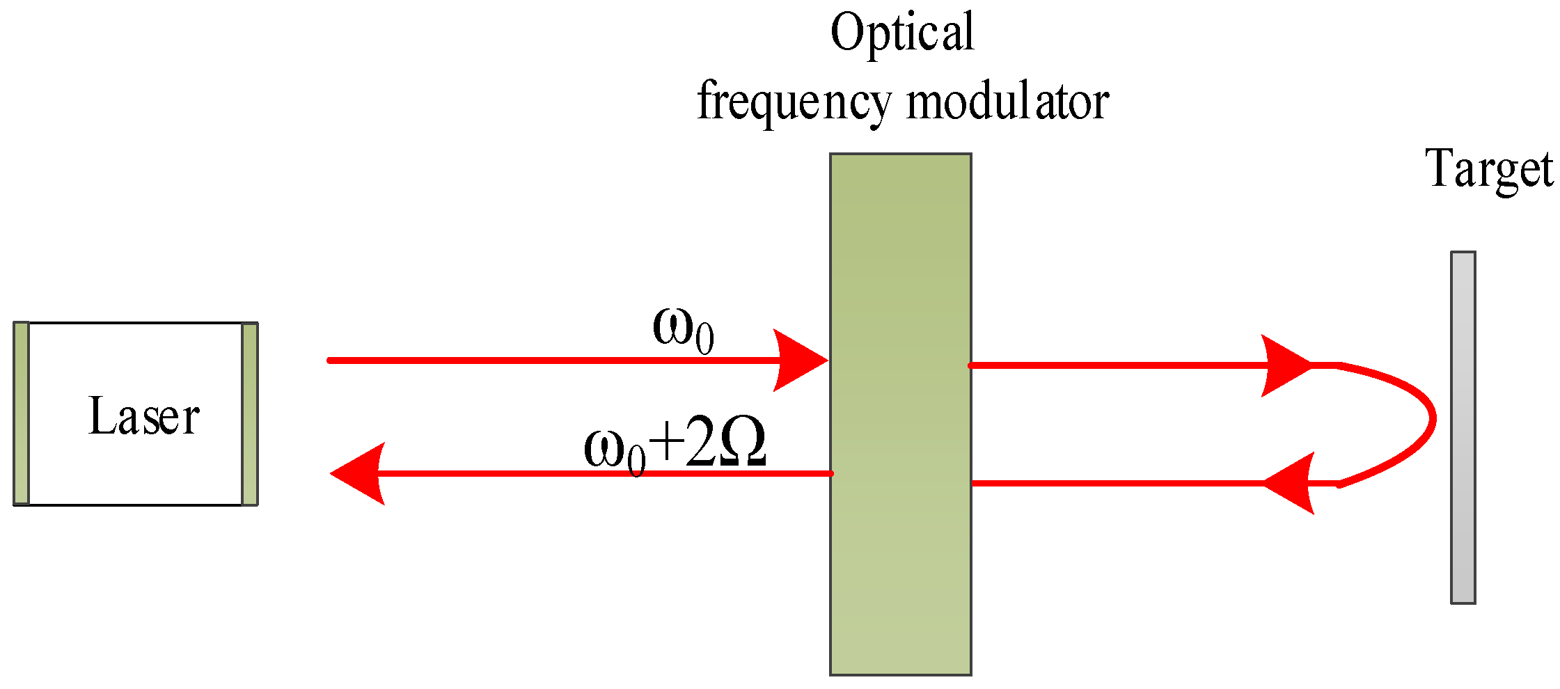
3.1. Sensing by Frequency-Shifted Optical Feedback

In 1999, Lacot et al. proposed an imaging method named laser optical feedback imaging (LOFI), where the optical frequency shift is resonant with the relaxation oscillation (RO) frequency of a solid-state laser [43]. In this case, the modulation of the laser intensity is highly sensitive to the reflectivity of the external target surface. Frequency-shifted feedback is usually applied to solid-state lasers because the RO frequency is around several hundred kHz, which can be easily achieved by using acousto-optical modulation, while for semiconductor lasers, it is hard to physically achieve due to the GHz-scale RO frequency. Figure 6 shows the basic structure of a frequency-shifted optical feedback laser system. When the frequency shift $\Omega$ is resonant with the RO frequency, the maximum relative modulation of the laser intensity is expressed as follows [43]:

$$\frac{\Delta P}{P}=2\frac{{\gamma }_c}{\eta {\gamma }_1}\sqrt{R_{{}_{eff}}},$$

(21)

where ${\gamma }_c$ is the laser cavity decay rate, ${\gamma }_1$ is the decay rate of the population inversion, $\eta$ is the normalized pumping rate. $R_{{}_{eff}}$ is the effective reflectivity of the target, and ${\gamma }_c/{\gamma }_1$ is typically on the order of ${10}^6$ for the solid-state laser. Therefore, once the proper frequency shift is set, the laser intensity can be greatly amplified. In [43], a two-dimensional image of a coin immersed in 1 cm of milk was obtained.

In 2001 [44], a 3D image of a toy was achieved by using the technology of frequency shift feedback together with a deformable liquid drop lens. After that, the frequency-shifted feedback technology was applied to traditional laser confocal tomography (LCT) and formed a technology called laser feedback confocal tomography, which shows superior characteristics compared with traditional LCT in terms of optical sensitivity and system stability [52]. To date, by using frequency-shifted optical feedback technology, different applications, including for the early detection of skin cancer [53], biological tissue imaging [54], the detection of ultrasound vibrations with nanometric amplitude [55], the inspection and location of foreign bodies in biological samples [56,57], the measurement of the refractive index [52], and structure measurement [58,59] have been reported.

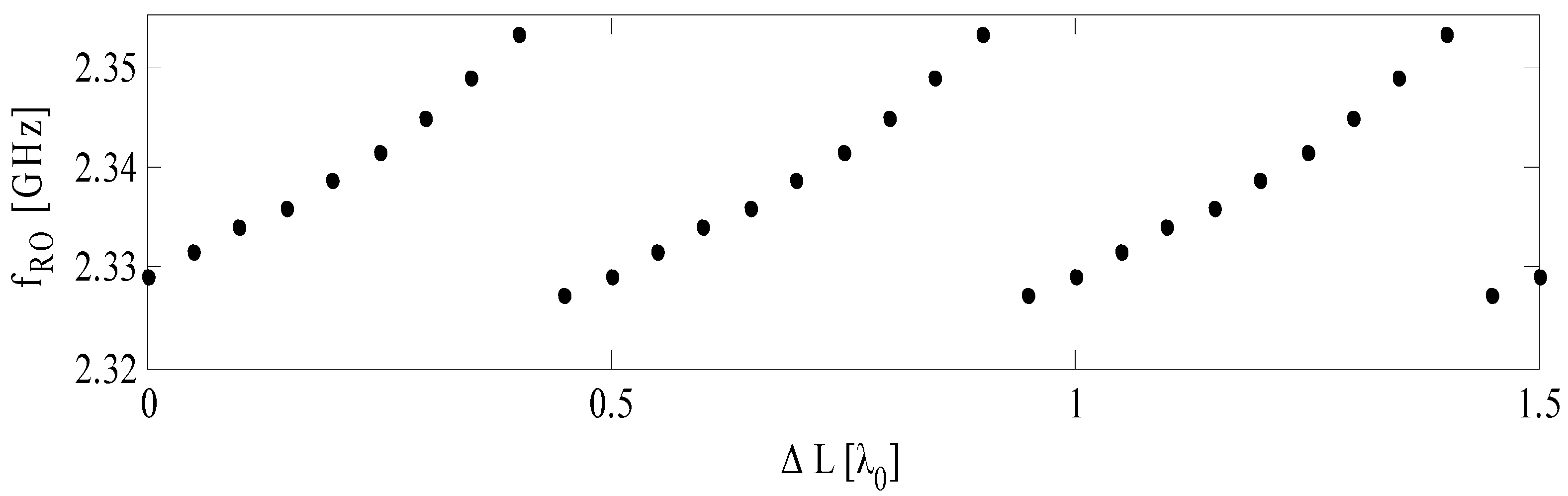
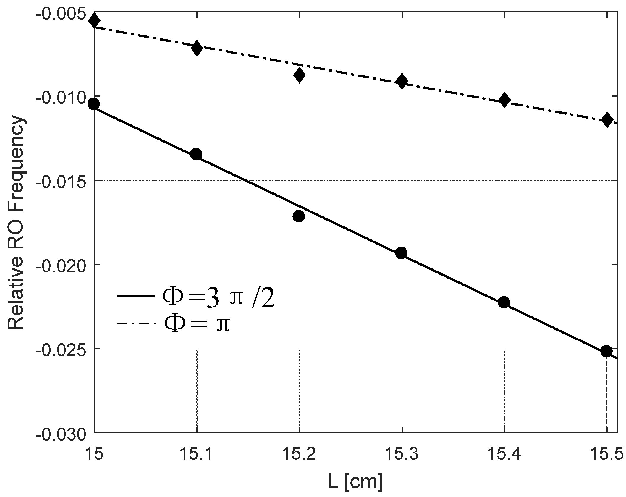
3.2. Sensing by Relaxation Oscillation Frequency

Relaxation oscillation in lasers occurs because the carrier cannot follow the photon decay rate [32]. An RO is easily able to be excited by a step input to the injection current, a shot noise originating from the driving circuit, and so on [39]. The RO frequency of lasers with EOF can be determined from system stability analysis [60,61]. Its value is often influenced by the laser’s operating conditions, including the injection current, feedback strength, and external cavity length [49]. Therefore, RO frequency can be utilized for sensing. To date, varieties of applications based on RO frequency have been developed.

In 2001, Lacot et al. [51] presented a work for imaging by using the RO frequency of a YAG microchip laser with weak EOF, where the RO frequency was modified by the reflectivity of the external target surface, as shown in Figure 7. Based on the relationship between RO frequency and target reflectivity, a 2D image of a French one franc coin was obtained. In 2009, based on precision measurement of RO frequency of the free running laser as a function of injection current, Kane et al. proposed a novel method of measuring the laser threshold current [62]. In 2013, Cohen et al. [63] presented a sub-laser-wavelength position sensing system using RO frequency of an LD with EOF, where the LD was set to operate in quasi-periodic oscillation. A displacement map between the variation of the RO frequency and two dimensional (2D) position (100 nm × 100 nm) was experimentally obtained, as shown in Figure 8, which shows the system can achieve an average 2D resolution of ~λ/160.

In 2017, Liu et al. [64] proposed a displacement sensing method by using the RO frequency of an LD with EOF operating at period-one oscillation, where the frequency of the period-one oscillation was considered as the RO frequency. Through numerically solving the L–K equations, the relationship between the RO frequency and external target displacement was investigated. The influence of the injection current on the LD and the initial external cavity length on the relationship were analyzed. It was found that the RO frequency varies with the displacement in a sawtooth-like form with the period of a half-laser wavelength, as shown in Figure 9. A micro-displacement sensing method was proposed based on this relationship. In 2018, a method of estimating the line-width enhancement factor (also called the $\alpha$ factor and Henry factor) of the LDs was presented by using the linear relationship between the RO frequency and external cavity length when the external cavity length has a variation much larger than the laser wavelength [65]. By carefully controlling the external cavity phase, two fitting curves corresponding to the phase of $\pi$ and $3\pi /2$ were able to be obtained, respectively, as shown in Figure 10. Dividing the gradients of these two fitting curves, the $\alpha$ factor was estimated. More recently, the relationship between the RO frequency and feedback optical phase with weak feedback strength was investigated and a new method for measuring the $\alpha$ factor of an LD was developed [20]. These RO frequency based methods of measuring the $\alpha$ factor have little in common with the conventional SMI-based methods, providing new option for measurement of the $\alpha$ factor, especially for lasers with small $\alpha$ factors.

3.3. Sensing by Dynamics in SMI Signals

In conversional SMI sensing applications, the laser operates in steady state and the modulated steady-state laser intensity is used as the sensing signal. An SMI system can operate in weak, moderate, or strong feedback regimes, according to the optical feedback level. In weak feedback regime, the laser is always in steady state and the SMI signals are closely sinusoidal. However, when the system operates in moderate or strong feedback regimes, the SMI signals exhibit a sawtooth-like pattern and some jumping points appear in the SMI signals. At the jumping or discontinuous points, transient damped oscillation corresponding to external cavity mode may happen [66]. On top of that, undamped RO may occur in moderate or strong feedback regimes [45,67], which may introduce high-level dynamics into the SMI signals. Figure 11 shows a simulated stability boundary for an SMI system with J = 1.3 Jth and L = 16 cm in the plane of feedback strength and optical phase by using the method in [68]. It finds that the stability boundary is periodic with respect to the variation of the optical phase with a period of 2π. The SMI system is in a steady state below the boundary, and it is unstable with undamped RO above the boundary.

In 2012, Teysseyre et al. [66] presented dynamics phenomenon in the sawtooth-like SMI signals where the target was more than one meter away from the LD when the RO was still damped. It was found that the damped oscillation in SMI signals contains information about the target distance and reflectivity, showing the possibility of estimating a target’s distance and reflectivity by using transient damped oscillation. In 2014, Fan et al. presented dynamic stability analysis on a laser SMI system and found some unique features of the SMI signals by simulation when the laser experienced undamped RO [42]. In 2016 [68], these features were experimentally verified and analyzed in detail, as shown in Figure 12. It has been found that a laser SMI systems in moderate or strong feedback regimes may operate with undamped RO, and the SMI signals in this case exhibit the form of high-frequency oscillation with amplitude modulated by a slow-varying signal. Interestingly, the slow-varying envelopes are similar to the conventional SMI signal characterized by the same fringe structure. The SMI signals in this condition have the potential for achieving sensing with improved sensitivity. Soon after this kind of SMI signal with period-one oscillation dynamics, a special case for the system with undamped RO was analytically modeled, and a method for displacement measurement with high resolution was proposed based on the model [69]. More recently, it was found that the signal noise ratio of SMI signals can be greatly improved by introducing an extra strong EOF into the system to make the laser operate in period-one oscillation [70]. By using the energy excited by period-one dynamics, the sensitivity of a laser SMI system is able to be largely enhanced.

3.4. Sensing by Laser Optical Chaos

When the feedback strength increases to certain values, lasers with EOF may exhibit chaos [49,60,61,71,72]. Laser optical chaos has been used in many applications, e.g., chaotic secure communication [49], random bit generators [73], photonic microwave signal generation [74], and optical logic computing [75], which was reviewed recently [76]. In this work, we focused on sensing applications based on optical chaos. Owing to the unique properties of laser chaos signals, e.g., short pulse width, rapid decorrelation due to irregular pulse intervals, and amplitudes, sensing by chaotic lasers has been proposed, e.g., chaotic radar [77], also known as chaotic lidar [78]. In 2001, ranging by using a chaotic laser pulse train generated by a semiconductor laser with EOF was developed and achieved a range resolution on the order of millimeters [79]. The measurement was made based on the shift of the peak in the correlation signal of the chaotic pulses when the target to be measured experienced a position change. Figure 13 shows the correlation of chaotic signals with different time delays that the light transmits to the target. After that, optical chaotic radar was intensively researched. In 2018, an unprecedented 3D-pulsed chaos lidar system to effectively improve energy-utilization efficiency and the corresponding signal-to-noise ratio was proposed [80]. More recently, a novel high-resolution chaos radar utilizing wideband chaos originated from a self-phase modulated optical feedback–based semiconductor laser cascaded by a dispersion component was introduced [81]. Simulation results show that the system can improve resolution and anti-interference characteristics significantly. Moreover, chaotic radars have also been applied in underwater target detection [82] and underwater 3D imaging [83].

Another kind of laser-chaos-based sensing application is chaotic correlation optical time domain reflectometer (OTDR). In 2008, laser chaos induced by EOF was developed for OTDR [84], where a spatial resolution of 6 cm was achieved for a distance of 140 m. Based on this, in 2012, Wang et al. achieved precise fault location with a resolution of 2 cm in a wavelength-division-multiplexing passive optical network by using a chaotic laser with adjustable wavelength [85]. In 2015, chaotic the OTDR technique was used for fiber attenuation measurement [86]. After that, different efforts were made for the chaotic OTDR to improve spatial resolutions and detection [87,88]. In addition, chaotic lasers are also used in Brillouin optical correlation domain analysis, i.e., the so-called chaotic BOCDA, which is a distributed optical fiber sensing technology based on stimulated Brillouin scattering (SBS) [89,90] In 2018, in order to suppress the off-peak amplification caused by chaotic autocorrelation sidelobes, a time-gated chaotic BOCDA was proposed and experimentally achieved with a 9 cm spatial resolution over a 10.2 km measurement range [90]. In 2021, a dual-slope-assisted chaotic Brillouin optical correlation domain analysis technology for static and dynamic strain measurement with high accuracy and resolution was proposed and experimentally demonstrated [89].

3.5. Transient Response of Lasers with EOF

For a laser with EOF, its dynamics and behavior are determined by both internal and external cavity–associated parameters, e.g., internal cavity round-trip time, line-width enhancement factor, injection current, feedback strength, external cavity length, etc. The internal parameters are fixed for a certain laser, but the external parameters can be varied in practice. By using L–K equations, we can numerically study the transient response of the system to a certain parameter. Figure 14 shows a simulation result for laser transient intensity and corresponding spectrum by numerically solving the L-K equations when the injection current (J) has a step change from 1.1 Jth to 1.3 Jth at 40 ns, where Jth is the threshold injection current of the solitary laser. Because the transient waveform and its spectrum contains the information of the system, the parameters related to the system, such as the line-width enhancement factor, can be retrieved by investigating the transient response.

4. Conclusions

This paper presents an overview on sensing by the dynamics of lasers with external optical feedback. Starting from the commonly used system, we introduce the operating principle of the laser system with external optical feedback. The derivation the L–K equations from the complex photoelectric-field equations is presented. Then the relative intensity noise of lasers with EOF and the modification of laser intensity induced by EOF was discussed. Afterwards, a few sensing applications by laser dynamics were categorized and reviewed, including sensing by frequency-shifted optical feedback, RO frequency, high-level dynamics in SMI signals, and laser optical chaos. Lastly, we presented the results of analyzing transient response lasers with EOF, indicating the feasibility of using them for sensing. With the development of laser technologies, e.g., the invention of nanolasers and terahertz lasers, it is believed that the dynamics of lasers with EOF will have more potential in sensing applications.

References

1. Lang, R.; Kobayashi, K. External optical feedback effects on semiconductor injection laser properties. IEEE J. Quantum Electron. 1980, 16, 347–355. [Google Scholar] [CrossRef]
2. Kleinman, D.; Kisliuk, P. Discrimination Against Unwanted Orders in the Fabry-Perot Resonator. Bell Syst. Tech. J. 1962, 41, 453–462. [Google Scholar] [CrossRef]
3. Rudd, M. A laser Doppler velocimeter employing the laser as a mixer-oscillator. J. Phys. E Sci. Instrum. 1968, 1, 723. [Google Scholar] [CrossRef]
4. Yu, Y.; Xi, J.; Chicharo, J.F. Measuring the feedback parameter of a semiconductor laser with external optical feedback. Opt. Express 2011, 19, 9582–9593. [Google Scholar] [CrossRef] [PubMed] [Green Version]
5. Yu, Y.; Xi, J.; Chicharo, J.F.; Bosch, T. Toward automatic measurement of the linewidth-enhancement factor using optical feedback self-mixing interferometry with weak optical feedback. IEEE J. Quantum Electron. 2007, 43, 527–534. [Google Scholar] [CrossRef] [Green Version]
6. Yu, Y.; Xi, J.; Chicharo, J.F.; Bosch, T.M. Optical Feedback Self-Mixing Interferometry with a Large Feedback Factor C: Behavior Studies. IEEE J. Quantum Electron. 2009, 45, 840–848. [Google Scholar] [CrossRef]
7. Lu, L.; Yang, J.; Zhai, L.; Wang, R.; Cao, Z.; Yu, B. Self-mixing interference measurement system of a fiber ring laser with ultra-narrow linewidth. Opt. Express 2012, 20, 8598–8607. [Google Scholar] [CrossRef]
8. Wu, S.; Wang, D.; Xiang, R.; Zhou, J.; Ma, Y.; Gui, H.; Liu, J.; Wang, H.; Lu, L.; Yu, B. All-Fiber Configuration Laser Self-Mixing Doppler Velocimeter Based on Distributed Feedback Fiber Laser. Sensors 2016, 16, 1179. [Google Scholar] [CrossRef] [Green Version]
9. Plantier, G.; Bes, C.; Bosch, T. Behavioral model of a self-mixing laser diode sensor. IEEE J. Quantum Electron. 2005, 41, 1157–1167. [Google Scholar] [CrossRef]
10. Zhu, K.; Guo, B.; Lu, Y.; Zhang, S.; Tan, Y. Single-spot two-dimensional displacement measurement based on self-mixing interferometry. Optica 2017, 4, 729–735. [Google Scholar] [CrossRef]
11. Khan, J.I.; Zabit, U. Sparsity Promoting Frequency Sampling Method for Estimation of Displacement and Self-Mixing Interferometry Parameters. IEEE Sens. J. 2021, 21, 10587–10594. [Google Scholar] [CrossRef]
12. Norgia, M.; Giuliani, G.; Donati, S. Absolute distance measurement with improved accuracy using laser diode self-mixing interferometry in a closed loop. IEEE Trans. Instrum. Meas. 2007, 56, 1894–1900. [Google Scholar] [CrossRef]
13. Zhao, Y.; Wang, C.; Zhao, Y.; Zhu, D.; Lu, L. An All-Fiber Self-Mixing Range Finder With Tunable Fiber Ring Cavity Laser Source. J. Lightwave Technol. 2021, 39, 4217–4224. [Google Scholar] [CrossRef]
14. Guo, D.; Wang, M. Self-mixing interferometry based on a double-modulation technique for absolute distance measurement. Appl. Opt. 2007, 46, 1486–1491. [Google Scholar] [CrossRef] [PubMed]
15. Guo, D.; Jiang, H.; Shi, L.; Wang, M. Laser self-mixing grating interferometer for MEMS accelerometer testing. IEEE Photon. J. 2018, 10, 1–9. [Google Scholar] [CrossRef]
16. Zhang, X.; Gu, W.; Jiang, C.; Gao, B.; Chen, P. Velocity measurement based on multiple self-mixing interference. Appl. Opt. 2017, 56, 6709–6713. [Google Scholar] [CrossRef]
17. Lin, K.; Yu, Y.; Xi, J.; Li, H.; Guo, Q.; Tong, J.; Su, L. A Fiber-Coupled Self-Mixing Laser Diode for the Measurement of Young’s Modulus. Sensors 2016, 16, 928. [Google Scholar] [CrossRef] [Green Version]
18. Wang, B.; Liu, B.; An, L.; Tang, P.; Ji, H.; Mao, Y. Laser Self-Mixing Sensor for Simultaneous Measurement of Young’s Modulus and Internal Friction. Photonics 2021, 8, 550. [Google Scholar] [CrossRef]
19. Yu, Y.; Giuliani, G.; Donati, S. Measurement of the linewidth enhancement factor of semiconductor lasers based on the optical feedback self-mixing effect. IEEE Photon. Technol. Lett. 2004, 16, 990–992. [Google Scholar] [CrossRef]
20. Liu, B.; Ruan, Y.; Yu, Y.; Wang, B.; An, L. Influence of feedback optical phase on the relaxation oscillation frequency of a semiconductor laser and its application. Opt. Express 2021, 29, 3163–3172. [Google Scholar] [CrossRef]
21. Zhao, Y.; Xiang, R.; Huang, Z.; Chen, J.; Lu, L. Research on the Multi-longitudinal mode laser self-mixing static angle-measurement system using a right-angle prism. Measurement 2020, 162, 107906. [Google Scholar] [CrossRef]
22. Wang, C.; Fan, X.; You, G.; Gui, H.; Wang, H.; Liu, J.; Yu, B.; Lu, L. Full-circle range and microradian resolution angle measurement using the orthogonal mirror self-mixing interferometry. Opt. Express 2018, 26, 10371–10381. [Google Scholar] [CrossRef] [PubMed]
23. Liu, B.; Ruan, Y.; Yu, Y. All-Fiber Laser-Self-Mixing Sensor for Acoustic Emission Measurement. J. Lightwave Technol. 2021, 39, 4062–4068. [Google Scholar] [CrossRef]
24. Bertling, K.; Perchoux, J.; Taimre, T.; Malkin, R.; Robert, D.; Rakić, A.D.; Bosch, T. Imaging of acoustic fields using optical feedback interferometry. Opt. Express 2014, 22, 30346–30356. [Google Scholar] [CrossRef] [Green Version]
25. Liu, B.; Ruan, Y.; Yu, Y.; Xi, J.; Guo, Q.; Tong, J.; Rajan, G. Laser self-mixing fiber Bragg grating sensor for acoustic emission measurement. Sensors 2018, 18, 1956. [Google Scholar] [CrossRef] [Green Version]
26. Wei, Y.; Huang, W.; Wei, Z.; Zhang, J.; An, T.; Wang, X.; Xu, H. Double-path acquisition of pulse wave transit time and heartbeat using self-mixing interferometry. Opt. Commun. 2017, 393, 178–184. [Google Scholar] [CrossRef]
27. Arasanz, A.; Azcona, F.J.; Royo, S.; Jha, A.; Pladellorens, J. A new method for the acquisition of arterial pulse wave using self-mixing interferometry. Opt. Lasers Technol. 2014, 63, 98–104. [Google Scholar] [CrossRef] [Green Version]
28. Norgia, M.; Pesatori, A.; Rovati, L. Self-mixing laser Doppler spectra of extracorporeal blood flow: A theoretical and experimental study. IEEE Sens. J. 2012, 12, 552–557. [Google Scholar] [CrossRef]
29. Annovazzi-Lodi, V.; Merlo, S.; Norgia, M. Measurements on a micromachined silicon gyroscope by feedback interferometry. IEEE/ASME Trans. Mechatron. 2001, 6, 1–6. [Google Scholar] [CrossRef]
30. Donadello, S.; Finazzi, V.; G Demir, A.; Previtali, B. Time-resolved quantification of plasma accumulation induced by multi-pulse laser ablation using self-mixing interferometry. J. Phys. D Appl. Phys. 2020, 53, 495201. [Google Scholar] [CrossRef]
31. Donadello, S.; Demir, A.G.; Previtali, B. Probing multipulse laser ablation by means of self-mixing interferometry. Appl. Opt. 2018, 57, 7232–7241. [Google Scholar] [CrossRef] [PubMed]
32. Lacot, E.; Day, R.; Stoeckel, F. Coherent laser detection by frequency-shifted optical feedback. Phys. Rev. A 2001, 64, 043815. [Google Scholar] [CrossRef]
33. Giuliani, G.; Norgia, M.; Donati, S.; Bosch, T. Laser diode self-mixing technique for sensing applications. J. Opt. A Pure Appl. Opt. 2002, 4, S283. [Google Scholar] [CrossRef] [Green Version]
34. Scalise, L.; Yu, Y.; Giuliani, G.; Plantier, G.; Bosch, T. Self-mixing laser diode velocimetry: Application to vibration and velocity measurement. IEEE Trans. Instrum. Meas. 2004, 53, 223–232. [Google Scholar] [CrossRef]
35. Donati, S. Developing self-mixing interferometry for instrumentation and measurements. Laser Photonics Rev. 2012, 6, 393–417. [Google Scholar] [CrossRef]
36. Taimre, T.; Nikolić, M.; Bertling, K.; Lim, Y.L.; Bosch, T.; Rakić, A.D. Laser feedback interferometry: A tutorial on the self-mixing effect for coherent sensing. Adv. Opt. Photonics 2015, 7, 570–631. [Google Scholar] [CrossRef]
37. Yu, Y.; Fan, Y.; Liu, B. Self-Mixing Interferometry and Its Applications. In Optical Design and Testing VII; Wang, Y.T., Ed.; SPIE: Bellingham, WA, USA, 2016; Volume 10021. [Google Scholar]
38. Li, J.; Niu, H.; Niu, Y.X. Laser feedback interferometry and applications: A review. Opt. Eng. 2017, 56, 050901. [Google Scholar] [CrossRef] [Green Version]
39. Ohtsubo, J. Semiconductor Lasers: Stability, Instability and Chaos; Springer: Berlin/Heidelberg, Germany, 2012. [Google Scholar]
40. Kallimani, K.I.; Mahony, M.J.O. Relative intensity noise for laser diodes with arbitrary amounts of optical feedback. IEEE J. Quantum Electron. 1998, 34, 1438–1446. [Google Scholar] [CrossRef]
41. Ju, R.; Spencer, P.S.; Shore, K.A. The relative intensity noise of a semiconductor laser subject to strong coherent optical feedback. J. Opt. B Quantum Semiclass. Opt. 2004, 6, S775–S779. [Google Scholar] [CrossRef]
42. Fan, Y.; Yu, Y.; Xi, J.; Guo, Q. Dynamic stability analysis for a self-mixing interferometry system. Opt. Express 2014, 22, 29260–29269. [Google Scholar] [CrossRef] [Green Version]
43. Lacot, E.; Day, R.; Stoeckel, F. Laser optical feedback tomography. Opt. Lett. 1999, 24, 744–746. [Google Scholar] [CrossRef] [PubMed]
44. Day, R.; Lacot, E.; Stoeckel, F.; Berge, B. Three-dimensional sensing based on a dynamically focused laser optical feedback imaging technique. Appl. Opt. 2001, 40, 1921–1924. [Google Scholar] [CrossRef]
45. Liu, B.; Wang, B.; Ruan, Y.; Yu, Y. Suppression of undamped relaxation oscillation in a laser self-mixing interferometry sensing system. Opt. Express 2022, 30, 11254–11265. [Google Scholar] [CrossRef] [PubMed]
46. Zhao, B.-B.; Wang, X.-G.; Zhang, J.; Wang, C. Relative intensity noise of a mid-infrared quantum cascade laser: Insensitivity to optical feedback. Opt. Express 2019, 27, 26639–26647. [Google Scholar] [CrossRef] [PubMed]
47. Yanhua, H.; Paul, J.; Spencer, P.S.; Shore, K.A. The effects of polarization-resolved optical feedback on the relative intensity noise and polarization stability of vertical-cavity surface-emitting lasers. J. Lightwave Technol. 2006, 24, 3210–3216. [Google Scholar] [CrossRef]
48. Petermann, K. External optical feedback phenomena in semiconductor lasers. IEEE J. Sel. Top. Quantum Electron. 1995, 1, 480–489. [Google Scholar] [CrossRef]
49. Uchida, A. Optical Communication with Chaotic Lasers: Applications of Nonlinear Dynamics and Synchronization; John Wiley & Sons: Hoboken, NJ, USA, 2012. [Google Scholar]
50. Donati, S.; Giuliani, G.; Merlo, S. Laser diode feedback interferometer for measurement of displacements without ambiguity. IEEE J. Quantum Electron. 1995, 31, 113–119. [Google Scholar] [CrossRef]
51. Lacot, E.; Day, R.; Pinel, J.; Stoeckel, F. Laser relaxation-oscillation frequency imaging. Opt. Lett. 2001, 26, 1483–1485. [Google Scholar] [CrossRef]
52. Zhou, B.; Wang, Z.; Shen, X. A New Method for Measuring Refractive Index with a Laser Frequency-shifted Feedback Confocal Microscope. Curr. Opt. Photon. 2020, 4, 44–49. [Google Scholar]
53. Mowla, A.; Du, B.W.; Taimre, T.; Be Rtling, K.; Rakić, A. Confocal laser feedback tomography for skin cancer detection. Biomed. Opt. Express 2017, 8, 4037. [Google Scholar] [CrossRef] [Green Version]
54. Hugon, O.; Paun, I.; Ricard, C.; Van der Sanden, B.; Lacot, E.; Jacquin, O.; Witomski, A. Cell imaging by coherent backscattering microscopy using frequency-shifted optical feedback in a microchip laser. Ultramicroscopy 2008, 108, 523–528. [Google Scholar] [CrossRef] [PubMed]
55. Girardeau, V.; Goloni, C.; Jacquin, O.; Hugon, O.; Inglebert, M.; Lacot, E. Nonlinear laser dynamics induced by frequency shifted optical feedback: Application to vibration measurements. Appl. Opt. 2016, 55, 9638–9647. [Google Scholar] [CrossRef] [PubMed] [Green Version]
56. Tan, Y.; Wang, W.; Xu, C.; Zhang, S. Laser confocal feedback tomography and nano-step height measurement. Sci. Rep. 2013, 3, 2971. [Google Scholar] [CrossRef] [PubMed]
57. Tan, Y.; Zhang, S.; Xu, C.; Zhao, S. Inspecting and locating foreign body in biological sample by laser confocal feedback technology. Appl. Phys. Lett. 2013, 103, 101909. [Google Scholar]
58. Wang, W.; Zhang, S.; Li, Y. Surface microstructure profilometry based on laser confocal feedback. Rev. Sci. Instrum. 2015, 86, 103108. [Google Scholar] [CrossRef]
59. Xu, C.; Tan, Y.; Zhang, S.; Zhao, S. The structure measurement of micro-electro-mechanical system devices by the optical feedback tomography technology. Appl. Phys. Lett. 2013, 102, 221902. [Google Scholar] [CrossRef]
60. Tromborg, B.; Osmundsen, J.H.; Olesen, H. Stability analysis for a semiconductor laser in an external cavity. IEEE J. Quantum Electron. 1984, 20, 1023–1032. [Google Scholar] [CrossRef]
61. Fan, Y.; Yu, Y.; Xi, J.; Guo, Q. Stability limit of a semiconductor laser with optical feedback. IEEE J. Quantum Electron. 2015, 51, 1–9. [Google Scholar] [CrossRef]
62. Kane, D.M.; Toomey, J.P. Precision Threshold Current Measurement for Semiconductor Lasers Based on Relaxation Oscillation Frequency. J. Lightwave Technol. 2009, 27, 2949–2952. [Google Scholar] [CrossRef]
63. Cohen, S.D.; Aragoneses, A.; Rontani, D.; Torrent, M.; Masoller, C.; Gauthier, D.J. Multidimensional subwavelength position sensing using a semiconductor laser with optical feedback. Opt. Lett. 2013, 38, 4331–4334. [Google Scholar] [CrossRef] [Green Version]
64. Liu, B.; Yu, Y.; Xi, J.; Guo, Q.; Tong, J.; Lewis, R.A. Displacement sensing using the relaxation oscillation frequency of a laser diode with optical feedback. Appl. Opt. 2017, 56, 6962–6966. [Google Scholar] [CrossRef] [PubMed]
65. Ruan, Y.; Liu, B.; Yu, Y.; Xi, J.; Guo, Q.; Tong, J. Measuring Linewidth Enhancement Factor by Relaxation Oscillation Frequency in a Laser with Optical Feedback. Sensors 2018, 18, 4004. [Google Scholar] [CrossRef] [PubMed] [Green Version]
66. Teysseyre, R.; Bony, F.; Perchoux, J.; Bosch, T. Laser dynamics in sawtooth-like self-mixing signals. Opt. Lett. 2012, 37, 3771–3773. [Google Scholar] [CrossRef] [PubMed] [Green Version]
67. Acket, G.A.; Lenstra, D.; Den Boef, A.; Verbeek, B. The influence of feedback intensity on longitudinal mode properties and optical noise in index-guided semiconductor lasers. IEEE J. Quantum Electron. 1984, 20, 1163–1169. [Google Scholar] [CrossRef]
68. Liu, B.; Yu, Y.; Xi, J.; Fan, Y.; Guo, Q.; Tong, J.; Lewis, R.A. Features of a self-mixing laser diode operating near relaxation oscillation. Sensors 2016, 16, 1546. [Google Scholar] [CrossRef] [PubMed] [Green Version]
69. Liu, B.; Ruan, Y.; Yu, Y.; Guo, Q.; Xi, J.; Tong, J. Modeling for optical feedback laser diode operating in period-one oscillation and its application. Opt. Express 2019, 27, 4090–4104. [Google Scholar] [CrossRef]
70. Ruan, Y.; Liu, B.; Yu, Y.; Xi, J.; Guo, Q.; Tong, J. High sensitive sensing by a laser diode with dual optical feedback operating at period-one oscillation. Appl. Phys. Lett. 2019, 115, 011102. [Google Scholar] [CrossRef]
71. Mørk, J.; Mark, J.; Tromborg, B. Route to chaos and competition between relaxation oscillations for a semiconductor laser with optical feedback. Phys. Rev. Lett. 1990, 65, 1999. [Google Scholar] [CrossRef]
72. Donati, S.; Fathi, M.T. Transition from short-to-long cavity and from self-mixing to chaos in a delayed optical feedback laser. IEEE J. Quantum Electron. 2012, 48, 1352–1359. [Google Scholar] [CrossRef]
73. Kanter, I.; Aviad, Y.; Reidler, I.; Cohen, E.; Rosenbluh, M. An optical ultrafast random bit generator. Nat. Phonton. 2010, 4, 58–61. [Google Scholar] [CrossRef]
74. Chan, S.C.; Hwang, S.K.; Liu, J.M. Period-one oscillation for photonic microwave transmission using an optically injected semiconductor laser. Opt. Express 2007, 15, 14921–14935. [Google Scholar] [CrossRef] [Green Version]
75. Chlouverakis, K.E.; Adams, M.J. Optoelectronic realisation of NOR logic gate using chaotic two-section lasers. Electron. Lett. 2005, 41, 359–360. [Google Scholar] [CrossRef]
76. Sciamanna, M.; Shore, K.A. Physics and applications of laser diode chaos. Nat. Phonton. 2015, 9, 151–162. [Google Scholar] [CrossRef] [Green Version]
77. Lin, F.-Y.; Liu, J.-M. Chaotic radar using nonlinear laser dynamics. IEEE J. Quantum Electron. 2004, 40, 815–820. [Google Scholar] [CrossRef]
78. Lin, F.-Y.; Liu, J.-M. Chaotic lidar. IEEE J. Sel. Top. Quantum Electron. 2004, 10, 991–997. [Google Scholar] [CrossRef]
79. Myneni, K.; Barr, T.A.; Reed, B.R.; Pethel, S.D.; Corron, N.J. High-precision ranging using a chaotic laser pulse train. Appl. Phys. Lett. 2001, 78, 1496–1498. [Google Scholar] [CrossRef]
80. Cheng, C.-H.; Chen, C.-Y.; Chen, J.-D.; Pan, D.-K.; Ting, K.-T.; Lin, F.-Y. 3D pulsed chaos lidar system. Opt. Express 2018, 26, 12230–12241. [Google Scholar] [CrossRef]
81. Feng, W.; Jiang, N.; Jin, J.; Zhao, A.; Zhang, Y.; Liu, S.; Qiu, K. High-Resolution Chaos Lidar Using Self-Phase-Modulated Feedback External-Cavity Semiconductor Laser-based Chaos Source. In Proceedings of 2021 19th International Conference on Optical Communications and Networks (ICOCN), Qufu, China, 23–27 August 2021; pp. 1–3. [Google Scholar]
82. Shen, Z.; Zhao, T.; Wang, Y.; Zheng, Y.; Shang, W.; Wang, B.; Li, J. Underwater target detection of chaotic pulse laser radar. Infrared Laser Eng. 2019, 48, 406004. [Google Scholar] [CrossRef]
83. Wang, B.; Guo, Z.; Shen, Z.; Xu, H.; Li, J. Underwater 3D Imaging Utilizing 520 nm Chaotic Lidar. J. Russ. Laser Res. 2020, 41, 399–405. [Google Scholar] [CrossRef]
84. Wang, Y.; Wang, B.; Wang, A. Chaotic correlation optical time domain reflectometer utilizing laser diode. IEEE Photon. Technol. Lett. 2008, 20, 1636–1638. [Google Scholar] [CrossRef]
85. Wang, A.; Wang, N.; Yang, Y.; Wang, B.; Zhang, M.; Wang, Y. Precise Fault Location in WDM-PON by Utilizing Wavelength Tunable Chaotic Laser. J. Lightwave Technol. 2012, 30, 3420–3426. [Google Scholar] [CrossRef]
86. Dong, X.; Wang, A.; Zhang, J.G.; Hong, H.; Wang, Y. Combined Attenuation and High Resolution Fault Measurements Using Chaos-OTDR. IEEE Photon. J. 2015, 7, 1–6. [Google Scholar] [CrossRef]
87. Li, M.; Zhang, X.; Zhang, J.; Zhang, M.; Qiao, L.; Wang, T. Long-Range and High-Precision Fault Measurement Based on Hybrid Integrated Chaotic Laser. Photonics Technol. Lett. IEEE 2019, 31, 1389–1392. [Google Scholar] [CrossRef]
88. Hu, Z.; Wang, B.; Wang, L.; Zhao, T.; Han, H.; Wang, Y.; Wang, A. Improving Spatial Resolution of Chaos OTDR Using Significant-Bit Correlation Detection. IEEE Photon. Technol. Lett. 2019, 31, 1029–1032. [Google Scholar] [CrossRef]
89. Zhao, L.; Wang, Y.; Hu, X.; Guo, Y.; Zhang, J.; Qiao, L.; Wang, T.; Gao, S.; Zhang, M. Improvement of Strain Measurement Accuracy and Resolution by Dual-Slope-Assisted Chaotic Brillouin Optical Correlation Domain Analysis. J. Lightwave Technol. 2021, 39, 3312–3318. [Google Scholar] [CrossRef]
90. Zhang, J.; Wang, Y.; Zhang, M.; Zhang, Q.; Li, M.; Wu, C.; Qiao, L.; Wang, Y. Time-gated chaotic Brillouin optical correlation domain analysis. Opt. Express 2018, 26, 17597–17607. [Google Scholar] [CrossRef]
Figure 1. Basic structure of a laser with external optical feedback.
Photonics 09 00450 g001
Figure 2. Basic model for a laser diode with external optical feedback.
Photonics 09 00450 g002
Figure 3. Simulated results for different dynamics of lasers with external optical feedback, (a) steady state, (b) period-one oscillation, (c) quasi-periodic oscillation, (d) chaotic oscillation.
Photonics 09 00450 g003
Figure 4. Relative intensity noise of a laser diode with EOF with J = 1.2 Jth, L = 25 cm.
Photonics 09 00450 g004
Figure 5. Power variation with different external reflectivity values.
Photonics 09 00450 g005
Figure 6. The basic structure a frequency-shifted feedback system, where ω 0 is the laser frequency, Ω is the frequency shift of the modulator.
Photonics 09 00450 g006
Figure 7. Experimental (symbols) and theoretical (dotted curve) evolution of the normalized RO frequency shift, where Δ f R O is the RO frequency width (adapted with permission from [51] © The Optical Society).
Photonics 09 00450 g007
Figure 8. The relationship between the quasi-periodic frequency shift and 2D displacement (adapted with permission from [63] © The Optical Society).
Photonics 09 00450 g008
Figure 9. The relationship between RO frequency and variation of external cavity length Δ L .
Photonics 09 00450 g009
Figure 10. Fitting curves of RO frequency for α measurement (adapted from [65]).
Photonics 09 00450 g010
Figure 11. SMI system stability boundary with the change of optical phase when J = 1.3 Jth, L = 16 cm.
Photonics 09 00450 g011
Figure 12. Experimental signals for DL4140-001S. (a) PZT control signal; (b) conventional SMI signals in steady state; (c) SMI signal containing period-one dynamics; (d) the laser intensity in the same condition as (c) when the target is stationary (adapted from [68]).
Photonics 09 00450 g012
Figure 13. Cross-correlation of chaotic signals with different time delays.
Photonics 09 00450 g013
Figure 14. Transient response of a laser with EOF when the injection current has a step change from 1.1 Jth to 1.3 Jth at 40 ns (a) laser intensity (b) the corresponding spectrum.
Photonics 09 00450 g014