Optical System Design of Oblique Airborne-Mapping Camera with Focusing Function

Abstract

The use of airborne-mapping technology plays a key role in the acquisition of large-scale basic geographic data information, especially in various important civil/military-mapping missions. However, most airborne-mapping cameras are limited by parameters, such as the flight altitude, working-environment temperature, and so on. To solve this problem, in this paper, we designed a panchromatic wide-spectrum optical system with a focusing function. Based on the catadioptric optical structure, the optical system approached a telecentric optical structure. Sharp images at different object distances could be acquired by micro-moving the focusing lens. At the same time, an optical passive compensation method was adopted to realize an athermalization design in the range of −40–60 °C. According to the design parameters of the optical system, we analyzed the influence of system focusing on mapping accuracy during the focusing process of the airborne-mapping camera. In the laboratory, the camera calibration and imaging experiments were performed at different focusing positions. The results show that the experimental data are consistent with the analysis results. Due to the limited experiment conditions, only a single flight experiment was performed. The results show that the airborne-mapping camera can achieve 1:5000 scale-imaging accuracy. Flight experiments for different flight altitudes are being planned, and the relevant experimental data will be released in the future. In conclusion, the airborne-mapping camera is expected to be applied in various high-precision scale-mapping fields.

1. Introduction

Airborne mapping is an important technical method of obtaining geographic information accurately and quickly. The use of this method can quickly obtain a large-scale and high-precision scale mapping of a target area in a short time and accurately obtain target plane coordinate information and elevation information on a map, which means it plays an important supporting role in digital city construction and land resource surveys [1,2]. In the field of surveying and mapping instruments, oblique airborne photography technology has challenged the traditional photography mode, which only allows photos to be taken from a single vertical angle. By obtaining image data information from different angles on the ground, combined with the high-precision position and orientation system (POS) that is equipped with the system, high-precision stereo-mapping products are obtained. The use of oblique photography technology can not only greatly improve the efficiency of the interpretation of surface features with airborne photography and 3D model production, but it can also provide a variety of direct measurement methods, such as distance, height, area, and volume calculation [3,4,5,6].

At present, Ultracam Osprey Mark 3 Premium, Penta-DigiCAM, RCD30, SWDC-5, TOPDC-5, ACM850, and VisionMap A3 are the typical airborne-mapping cameras with advanced performance [7]. These mapping cameras, except VisionMap A3, adopt the multi-lens image mosaic method, and the focal lengths are all less than 150 mm. VisionMap A3 is a new generation of the step-scan-imaging digital airborne camera produced by VisionMap Company (Tel Aviv, Israel). VisionMap A3 is a long-focal camera with two lenses which have 300 mm focal lengths. The two lenses are placed parallel to the flight direction, and the image data are obtained via scanning imaging, which means VisionMap A3 has an ultra-high data acquisition capability, image resolution, and operational efficiency.

The above-mentioned mapping cameras have made many contributions in the field of surveying and mapping. But they all adopt fixed-focus structures. The main factor is that the system focusing changes the camera’s interior orientation elements, which reduces the mapping accuracy. With the development of airborne-mapping technology, the requirements for mapping cameras have been increased further. Mapping cameras are required to be able to achieve high-precision scale mapping within the range of object distances from 1 km to infinity. However, the fixed-focus optical system cannot clearly photograph a target area with a large depth of field, and the defocusing application reduces the imaging quality, thus affecting the mapping accuracy [8]. To enable an airborne-mapping camera to produce high-precision scale mapping in a wide range of dynamic object distances, a mapping camera with a focusing function which has minimal influence on mapping accuracy is urgently needed. However, at present, no effective work has been carried out regarding oblique airborne-mapping cameras with focusing functions.

The rest of this article is organized as follows. In Section 2, we analyze the main technical indicators of the airborne-mapping camera, and the analysis results offer the parameter bounds for the optical design in Section 3. Section 3 shows the optical design of the airborne-mapping camera, and then, the analysis of the effect of the working-environment temperature on image quality and interior orientation elements is presented. In Section 4, the effect of system focusing on image quality and interior orientation elements is analyzed. In Section 5, the real experimental process is presented, and the results are discussed. Section 6 shows the conclusions.

2. Main Technical Indicators and Decomposition of Airborne-Mapping Cameras

2.1. Technical Requirements of Airborne Mapping Cameras

Compared with spaceborne-mapping cameras, airborne-mapping cameras have the advantage of being able to realize large-scale surveying and mapping in a short time period. Additionally, large mapping scales require higher imaging resolutions, meaning airborne-mapping cameras require high imaging resolutions. Compared with airborne reconnaissance cameras, airborne-mapping cameras can achieve the accurate measurement of ground targets, and at the same time, they also place strict requirements on the accuracy of geometric parameters which affect the accuracy of surveying and mapping. The main technical indicators of the airborne-mapping camera studied in this paper are listed in

Table 1. Main technical indicators of the airborne-mapping camera.

Parameters	Values
Wavelength	435–900 nm
Flight altitude	1–7.5 km
Scanning range	±60°
Modulation transfer function (MTF)	≥0.2 (80 lp/mm at whole field of view (fov))
Mapping scale	1:5000

. We mounted the oblique airborne-mapping camera on a stable platform. By controlling the scanning angle of the stable platform, various working modes of the oblique airborne-mapping camera, such as vertical downward views/oblique views, ±60° full-amplitude scanning, and interval scanning, could be realized, as shown in Figure 1.

2.2. Requirements of Mapping Scale for the Ground Sample Distance (GSD)

According to the main technical indicators of the above-mentioned oblique airborne-mapping camera, the oblique airborne-mapping camera needed to achieve the national-standard-mapping accuracy of 1:5000, which required the GSD of the camera. According to the basic specifications for surveying and mapping of national fundamental scale maps (GB 35650-2017), the GSD required by specifications for the mapping camera are given in

Table 2. GSD of the airborne-mapping camera.

Scale Imaging Accuracy	GSD/m
1:2000	≤0.20
1:5000	≤0.50

.

In this paper, the oblique airborne-mapping camera had a CMOS-imaging sensor with a 5120 × 3840 array and a pixel size of 6.4 μm. It had a maximum working altitude of 7.5 km and a maximum working inclination of 60°. Figure 2 shows the schematic of the focal length calculation. Since the pixel size is much smaller than the focal length, the angle, $\beta$, approaches 90° infinitely.

The formula for calculating the focal length of the optical system is given as follows. To meet the requirement that the GSD was not less than 0.5 m, the focal length, $f$, needed to be greater than 384 mm. Considering the design margin, the focal length was set to 450 mm.

$$f = \left(\raisebox{1ex}{$h/{\cos }^2 {60}^{\circ }$}\!\left/ \!\raisebox{-1ex}{$GS{D}_{{60}^{\circ }}$}\right.\right) \times ps,$$

(1)

where $h$ is the flight altitude, and $ps$ is the pixel size of the CMOS-imaging sensor.

2.3. Requirements of Mapping Scale for the Interior Orientation Element Accuracy

High-precision-mapping products have high requirements in terms of the plane accuracy and elevation accuracy of photogrammetry [9,10]. To achieve 1:5000 scale-mapping accuracy, according to the terrain category, the plane accuracy and elevation accuracy have different accuracy requirements. According to the basic specifications for surveying and mapping of national fundamental scale maps (GB 35650-2017), the specific accuracy requirements are shown in

Table 3. Ground location accuracy of the airborne-mapping camera.

Scale-Imaging Accuracy	Terrain Category	Plane Accuracy/m	Elevation Accuracy/m
1:2000	Flat grounds	1.2	0.40
	Hills	1.2	0.50
	Mountains	1.6	1.20
	High mountains	1.6	1.50
1:5000	Flat grounds	2.5	0.50
	Hills	2.5	1.20
	Mountains	3.75	2.50
	High mountains	3.75	4.00

.

The oblique airborne-mapping camera adopts the principle of stereo imaging. The calibration accuracy of interior orientation elements and exterior orientation elements directly affect the plane accuracy and elevation accuracy of photogrammetry. Considering that the optical system design of an oblique airborne-mapping camera is mainly discussed in this paper, only the influence of the camera’s interior orientation elements on the ground location accuracy are discussed here, while the influence of the camera’s exterior orientation elements is not discussed.

Based on the error propagation law, the photogrammetric forward intersection method, combined with the technical ability of our design, installation, and calibration, we decomposed the plane accuracy and elevation accuracy in the 1:5000 scale-mapping accuracy [11,12,13]. The specific indicator decomposition process is not presented in this paper. The indicators decomposed into interior orientation element errors are shown in

Table 4. Indicators decomposed into interior orientation elements errors.

Interior Orientation Elements	Composition	Value/μm
Calibrated principal distance measurement error	$m_{f1}$	3
	$m_{f2}$	≤8
	$m_{f3}$	≤10
Principle point measurement error	$m_{p1}$	3
	$m_{p2}$	≤2
	$m_{p3}$	≤2

. According to the characteristics of the optical system in this paper, the factors that affect the interior orientation element accuracy include camera calibration, working-environment temperature, and system focusing. Namely, the measurement error of the calibrated principal distance, $m_f$, is composed of the calibration error of the calibrated principal distance, $m_{f1}$, environment-introduced error, $m_{f2}$, and repeated positioning errors introduced by system focusing, $m_{f3}$. In addition, the measurement error of the principle point, $m_p$, consists of the calibration error of the principle point, $m_{p1}$, environment-introduced error, $m_{p2}$ and repeated positioning errors introduced by system focusing, $m_{p3}$. The camera-calibration accuracy in our laboratory is shown in Table 4. The subsequent analysis results all met the requirements outlined in Table 4.

3. Optical System Design of the Oblique Airborne-Mapping Camera

3.1. Optical System Parameters

Based on the main technical indicators and analysis in Section 2, the optical system parameters are shown in

Table 5. Parameters for the optical system of the airborne-mapping camera.

Parameters	Values
Wavelength	435–900 nm
Focal length	450 mm
Diagonal image size	40.96 mm
F-number	4.2
Maximum relative distortion	≤0.1%
MTF	≥0.2 (80 lp/mm at whole fov and different focusing positions)
Pixel size	6.4 μm
Telecentric angle	≤0.1°
Back focal length	≥12 mm
Total length	≤265 mm

.

3.2. Configuration Design of the Optical System

Based on the catadioptric optical structure, the optical system approached a telecentric optical structure, and the telecentric angle was less than 0.1°. The two-mirror telescope systems had R-C structures. A correction lens group was inserted between the secondary mirror and the focal plane to enlarge the system’s fov. The correction lens group contained a set of air-spaced doublets, which was used to correct the chromatic aberration introduced by a wide-range spectrum. The TF3 special glass was used to correct the secondary spectrum [14,15,16,17,18]. A positive lens was set close to the image surface to control the incident angle of the chief ray. The last lens was set as the focusing lens, and the large-depth-of-field-imaging effect of the optical system was realized with micro-movements on the lens axis [19,20]. The athermalization design of the optical system was realized by matching the optical materials and the structural materials [21,22,23]. The optical system in the oblique airborne-mapping camera was optimized using CODEV software. The final design result is shown in Figure 3.

3.3. Environmental Adaptability

The influence of the airborne-working-environment temperature changed the curvature radius and refractive index of the optical components, which affected the focal length of the optical system. Changes in the focal length caused the system to defocus and caused changes in the interior orientation element parameters, which affected the mapping accuracy. Therefore, it was necessary to carry out an environmental adaptability analysis and realize the athermalization design of the optical system. This type of design enabled wide-range temperature adaptability in the optical system through the selection of a combination of glass materials with positive and negative photo-thermal expansion rates and the selection of air-gap-structure materials.

In the temperature range of −40–60 °C, the MTF of the optical system was better than 0.2 (80 lp/mm at whole fov), which did not require temperature focusing and had little influence on the image quality. The MTF curves plotted for different positions on the diagonal of the sensor at different temperatures are shown in Figure 4.

As the whole optical system was designed with rotational symmetry, the location of the camera’s principal point did not change when the camera worked in a stable environment. Therefore, the environment-introduced error, $m_{p2}$, was 0 µm. In addition, the calibrated principal distance errors introduced by different temperatures are shown in Figure 5. In the working-environment temperature range of −40–60 °C, the environment-introduced error, $m_{f2}$, was 4.5 µm, which met the requirement outlined in Table 4.

4. Analysis of the Influence of System Focusing on Mapping Accuracy

4.1. Analysis of the Influence of System Focusing on Image Quality

The system defocus causes the MTF to degrade as follows [24]:

$$MT{F}_{Defocus} = \raisebox{1ex}{$2J_1(\mathrm{X})$}\!\left/ \!\raisebox{-1ex}{$\mathrm{X}$}\right.,$$

(2)

$$\mathrm{X} = \pi {\nu }_n(\raisebox{1ex}{$\mathrm{\Delta }l$}\!\left/ \!\raisebox{-1ex}{$F-number$}\right.),$$

(3)

where $J_1(\mathrm{X})$ is the first-order Bessel function, $\mathrm{\Delta }l$ is the defocus amount, $F-number$ is the inverse of the relative aperture, and ${\nu }_n$ is the cut-off frequency.

It can be seen from the formula outlined above that with changes in the object distance, the image plane is defocused, resulting in a decline in image quality. Figure 6 shows the MTF-defocus amount curve of the optical system. When the defocus amount was within ±0.04 mm, the MTF of the whole field of view of the optical system was not less than 0.2, and the system could photograph clearly. In addition, according to Newton’s formula for paraxial-imaging systems, when the defocus amount was 0.045 mm, the object distance corresponding to the system was 4500 m, and the static MTF of the edge field of view of the optical system was 0.2 at 80 lp/mm. To meet the requirement that the static MTF of the optical system was not less than 0.2, the system needed to focus when the object distance was within a distance of 1000 m to 4500 m.

Considering the flight altitude, the image-motion-compensation capability and imaging range at different object distances for the oblique airborne-mapping camera, a six-level-focusing method was proposed in this paper, as shown in

Table 6. Imaging range of optical system after focusing with different ranges.

Focusing Position	Object Distance/km	Imaging Range/km	Scanning Range/°
1	Inf	4.5 km~inf	±60
2	3	2–9	±60
3	2.5	1.8–5.5	±60
4	2	1.5–4.2	±60
5	1.5	1–2.5	±53
6	1	0.8–1.3	±39

. Criterion of depth of field in this paper is that the MTF is not less than 0.2. In addition, we show that the camera can auto-focus based on the inertial measurement unit (IMU) height information.

It can be seen from Table 6 that when the flight altitude was higher than 2km, the oblique airborne-mapping camera could ensure excellent imaging within the ±60° scanning range by focusing once on the target scene. However, when the flight altitude was lower than 2 km, the scanning range needed to be reduced as appropriate. Taking the object distance of 1 km as an example, the optical system had an excellent imaging range of 0.8 km to 1.3 km, which could only achieve clear imaging of the ±39° scanning range. It can be seen from Figure 7 that the system only needed to focus once within the ±39° scanning range without real-time focusing.

4.2. Analysis of the Influence of System Focusing on Interior Orientation Elements

When an airborne-mapping camera photographs target areas with different object distances, it needs to focus, and the change in the focusing-lens position causes the calibrated principal distance to change, which affects the accuracy of photogrammetry. Figure 8a shows the variation in the calibrated principal distance at different focusing positions. To reduce the influence of the change in focusing lens position on the calibrated principal distance, we calibrated the airborne-mapping camera at different focusing positions. Additionally, the calibration value of the focal length at different focusing positions was used as the calibrated principal distance of the interior orientation element for measurement to reduce the influence of the focal length error on the mapping accuracy. According to the camera-calibration accuracy in our laboratory, the measurement results would not be affected. Figure 8b shows the influence of repeated focusing-positioning accuracy on the calibrated principal distance error. According to the existing focusing technology, the repeated positioning accuracy was set to 3 μm, and the repeated positioning errors introduced by focusing, $m_{f3}$, was 7.5 μm, which met the requirements outlined in Table 4.

In the process of moving back and forth, the focusing lens will inevitably be eccentric and tilted, which will affect the location of the principle point of interior orientation elements. The principal point location error at different decenters and tilt errors is shown in Figure 9.

As can be seen from Figure 8, to ensure the stable accuracy of the principal point location of the interior orientation elements in the mapping camera, the repeated positioning errors introduced by focusing, $m_{p3}$, should not be greater than 2 µm. Combined with the existing lens-assembly process, the decenter error of the focusing lens should be better than 5 µm, and the tilt error of the focusing lens should be better than 20 arcseconds.

5. Real Experiment

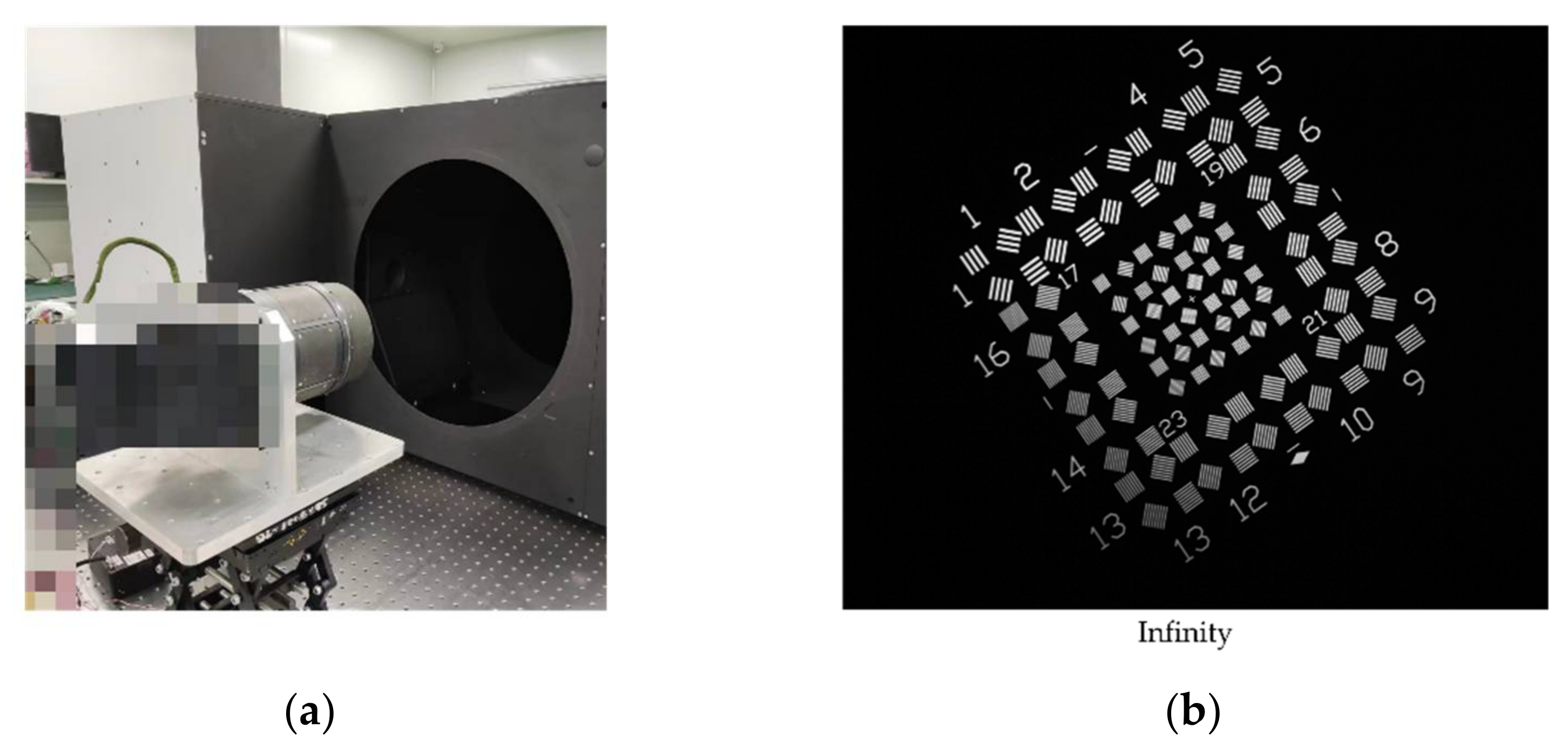
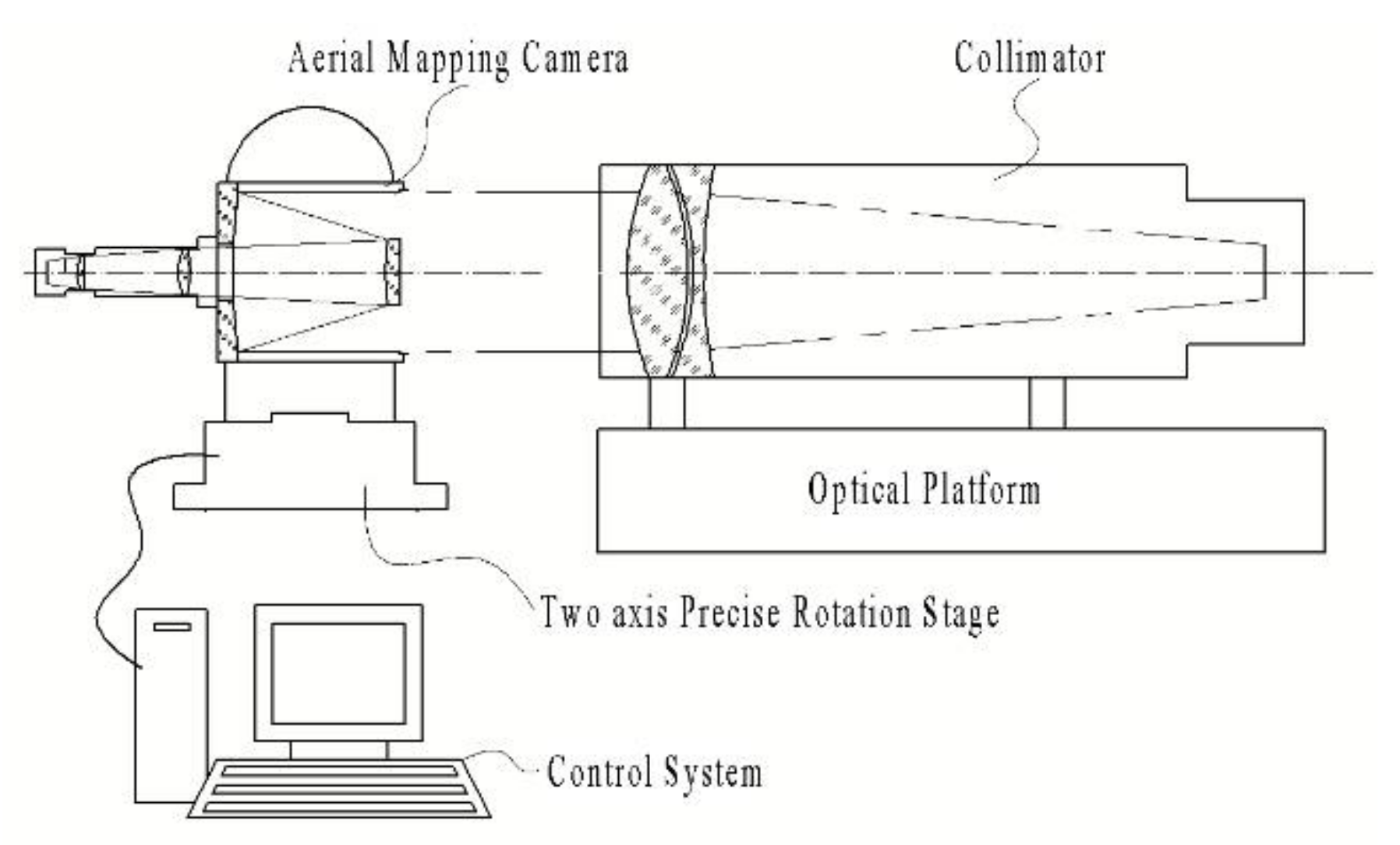
5.1. Pixel Resolution Experiment in Laboratory

To adequately assess the pixel resolution indicator at different focusing positions of the oblique airborne-mapping camera, an experimental platform was built, as shown in Figure 10. The airborne-mapping camera was fixed on a six-degrees-of-freedom (6-DOF) platform and placed in front of a collimator. The optical axes of the airborne-mapping camera and the collimator could be made coaxial by adjusting the 6-DOF platform. By adjusting the focal plane of the collimator, which could simulate the target of different object distances, the focusing positions and their imaging range were calibrated and validated in the laboratory. The patterns of resolution target in the collected images were interpreted, and the distinguishable group numbers were recorded. Figure 11a shows the real experiment system setup. Taking the infinity target as an example, Figure 11b shows the experiment result in terms of resolution target.

The calculation formula of the line pairs per millimeter that the mapping camera can distinguish can be obtained as follows:

$$N = \frac{N_0}{f}{f}_0,$$

(4)

where $N_0$ is the number of distinguishable line pairs per millimeter on the resolution target. In this experiment, the 20th group of No. 4 resolution target was selected, and its value is 18.7 lp/mm. $f_0$ is the focal length of the collimator, and its value is 2000 mm.

According to the formula presented above, the number of line pairs per millimeter that the camera can distinguish is 83 lp/mm, which reach the design value.

5.2. Interior Orientation Element Calibration Experiment in Laboratory

The precise angle measurement method was used to calibrate the interior orientation elements in the mapping camera. The mapping camera was fixed on a two-axis precision turntable to photograph the star-point target passing through the collimator. By adjusting the camera attitude, it was ensured that the star-point target was always photographed on a horizontal/vertical line of pixels on the detector focal plane when the turntable rotated at the horizontal/vertical fov. An experimental platform was built, as shown in Figure 12. By adjusting the two-axis precision turntable to change the incident angle of parallel light, the star-point images at different incident angles were obtained. At the same time, the turntable angle values and the star-point image locations were recorded [25,26]. Figure 13 shows the real scene and the star-point image of the interior orientation element calibration experiment. The distortion values along the X-direction and Y-direction can be expressed as

$$\begin{array}{c}\mathrm{\Delta }{x}_{i,j} = (x_{i,j} - x_0)d - f\left(\raisebox{1ex}{$\tan {\alpha }_i$}\!\left/ \!\raisebox{-1ex}{$\cos {\beta }_j$}\right.\right),\\ \mathrm{\Delta }{y}_{i,j} = (y_{i,j} - y_0)d - f\tan {\beta }_j,\\ q_{\max } = \max \left\{\frac{\sqrt{{\left(\mathrm{\Delta }{x}_{i,j}\right)}^2 + {\left(\mathrm{\Delta }{y}_{i,j}\right)}^2}}{h_0}\right\},\end{array}$$

(5)

where $\mathrm{\Delta }{x}_{i,j}$ ($\mathrm{\Delta }{y}_{i,j}$) is the distortion values along the X-direction (Y-direction) of the camera, $x_{i,j}$ ($y_{i,j}$) is the pixel coordinate value of the collected star-point image along the X-direction (Y-direction), $x_0$ ($y_0$) is the coordinate value of the camera principle point along the X-direction (Y-direction), $d$ is the pixel size of the camera detector, ${\alpha }_i$ is the azimuth angle value of the turntable at the ith test point planned along the X-direction of the camera, ${\beta }_j$ is the pitch angle value of the turntable at the jth test point planned along the Y-direction of the camera, $q_{\max }$ is the maximum relative distortion value of the whole fov, and $h_0$ is the theoretical image height.

In the process of interior orientation element calibration, a total of $n \times n$ calibration points were obtained. Taking the least squares fit of the whole fov distortion values as the constraint condition, the calculation equation of the interior orientation elements was established, given by

$$\min \left({\displaystyle \sum _{i = 1}^{n_x}{\displaystyle \sum _{j = 1}^{n_y}\left(\mathrm{\Delta }{x}_{i,j}{}^2 + \mathrm{\Delta }{y}_{i,j}{}^2\right)}}\right),$$

(6)

The formula presented above is a function of $x_0$, $y_0$, and $f$, and the interior orientation elements could be obtained by taking the partial derivative with respect to $x_0$, $y_0$, and $f$.

$$\begin{array}{l}\frac{\partial \left({\displaystyle \sum _{i = 1}^{n_x}{\displaystyle \sum _{j = 1}^{n_y}\left(\mathrm{\Delta }{x}_{i,j}{}^2 + \mathrm{\Delta }{y}_{i,j}{}^2\right)}}\right)}{\partial x_0} = 0,\\ \frac{\partial \left({\displaystyle \sum _{i = 1}^{n_x}{\displaystyle \sum _{j = 1}^{n_y}\left(\mathrm{\Delta }{x}_{i,j}{}^2 + \mathrm{\Delta }{y}_{i,j}{}^2\right)}}\right)}{\partial y_0} = 0,\frac{\partial \left({\displaystyle \sum _{i = 1}^{n_x}{\displaystyle \sum _{j = 1}^{n_y}\left(\mathrm{\Delta }{x}_{i,j}{}^2 + \mathrm{\Delta }{y}_{i,j}{}^2\right)}}\right)}{\partial f} = 0\end{array}$$

(7)

By bringing $x_0$, $y_0$, and $f$ into Equation (5), the maximum relative distortion value of the whole fov could be obtained. And according to the polynomial difference, the distortion value of each pixel in the planar array camera could also be obtained. Then, the camera’s interior orientation elements at six different focusing positions were calibrated using the same method mentioned above. The calibration results are shown in

Table 7. The calibration results of the interior orientation elements.

Focusing Position	$\mathit{n} \times \mathit{n}$	${\mathit{x}}_0/\mathbf{mm}$	${\mathit{y}}_0/\mathbf{mm}$	$\mathit{f}/\mathbf{mm}$	${\mathit{q}}_{\mathbf{max}}$
1	15 × 15	16.395	12.276	450.145	0.02%
2	15 × 15	16.388	12.278	449.064	0.04%
3	15 × 15	16.383	12.291	448.828	0.03%
4	15 × 15	16.389	12.295	448.536	0.05%
5	15 × 15	16.393	12.283	447.944	0.04%
6	15 × 15	16.386	12.279	446.937	0.06%

.

It can be seen from Table 7 that after focusing, the principal point, calibrated principal distance, and maximum distortion value of the optical system were consistent with the analysis results, which could meet the requirements of high-precision-mapping photography. At the same time, it can be seen from Table 7 that the repeated positioning accuracy and the adjustment accuracy of the focusing mechanism could meet the design requirements.

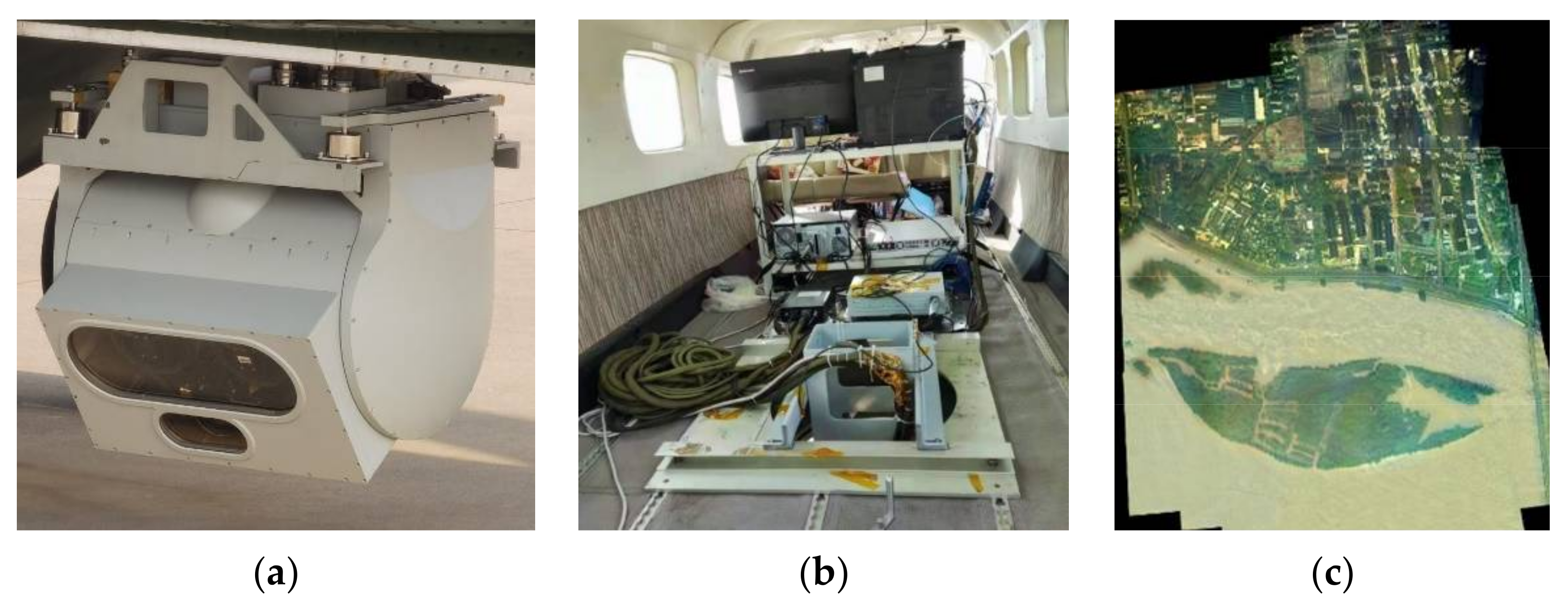
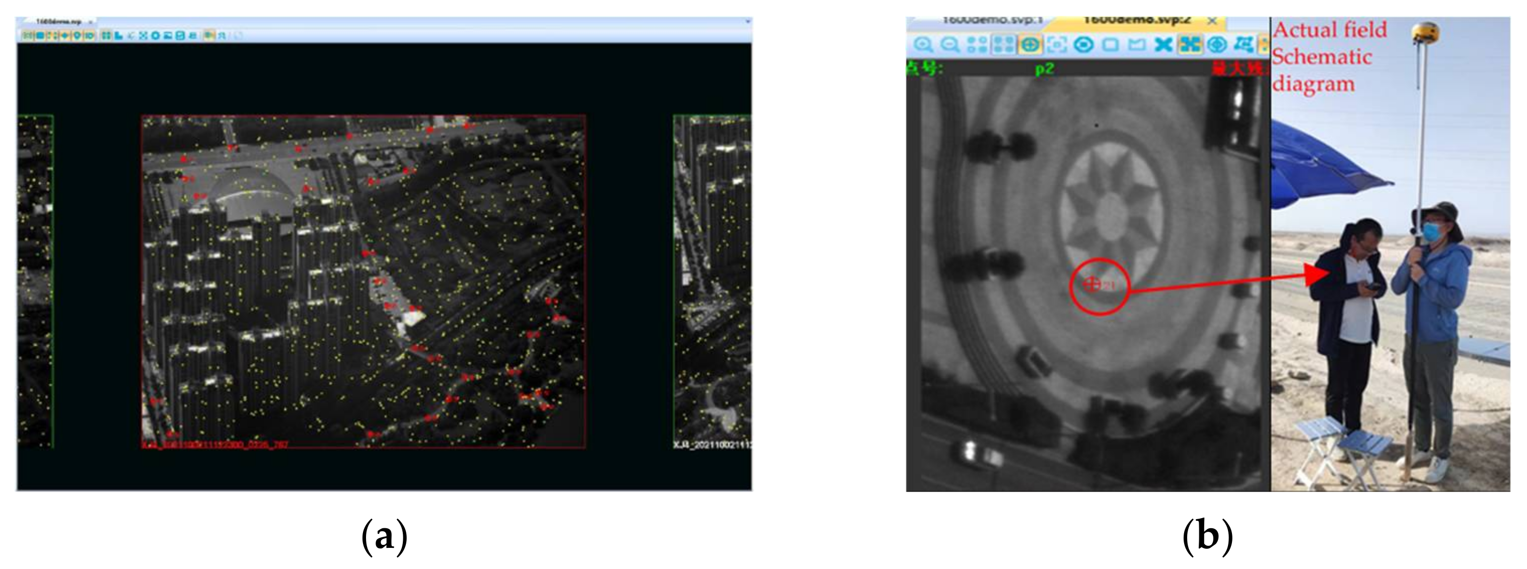
5.3. Flight Experiment with Real Data

To verify the 1:5000 scale-mapping-accuracy indicator of the designed oblique airborne-mapping camera, a flight experiment based on real data was carried out. Firstly, we fixed the airborne-mapping camera calibrated with the interior orientation elements on a two-axis stable platform and calibrated the exterior orientation elements. The results are shown in

Table 8. Parameters in experiments with the airborne-mapping camera.

Parameters	Values
Flight altitude	3.17 km
Flight speed	242 km/h
Scanning range	±60°
Typical exposure time	0.5 ms
Accuracy of the stable platform	<35 urad (PV-value)

. Then, we chose an area of 10 km² and conducted a flight experiment. The parameters were set as shown in Table 8, including the flight altitude, flight speed, the exposure time, and the stable platform accuracy. The average height of the ground in the experiment area was 70 m, which was the plane area. The focusing position was set to 2, according to the flight altitude in Table 8 and the object distance in Table 6. Figure 14 shows the real scene and the mosaic image of the flight experiment. According to the parameters of the flight experiment, the GSD calculation formula was obtained by transforming Equation (1), which was less than 0.18 m after calculation.

$$GS{D}_{{60}^{\circ }} = \left(\raisebox{1ex}{$h/{\cos }^2 {60}^{\circ }$}\!\left/ \!\raisebox{-1ex}{$f$}\right.\right) \times ps,$$

(8)

The airborne-mapping camera equipped with the POS system was used to perform an uncontrolled block adjustment on the scanned image of the flight area. There were 30 precision measuring points placed on the ground. The measuring points were distributed at clear signs, such as roads, intersections and so on. These points were measured using the global navigation satellite system (GNSS) real time kinematic (RTK) method [27,28]. The measuring equipment was composed of survey-grade GNSS I70 receivers made by CHCNAV. The position accuracy of the points was at the centimeter level. By comparing the object coordinates of the measuring points measured in the image with those measured with a GPS in the actual field, the difference between them was calculated. Figure 15a shows the distribution of the tie points, which are shown as green, and the measuring points, which are shown as red in the area. Figure 15b shows the comparison of the experiment results. The statistical results show that the plane errors of these checkpoints were all less than 0.8 m, and the elevation errors were all less than 0.3 m. According to the basic specifications for surveying and mapping of national fundamental scale maps (GB 35650-2017), the aerotriangulation of images in this experiment area met the requirements of the 1:2000 scale-mapping accuracy, which could meet the 1:5000 scale-mapping accuracy at a photographic distance of 15 km.

Due to the limited time and the authorized flight height, the conducted experiment had verified the focusing position 2 and its mapping accuracy. More flight experiments have been planned; verifications for other focusing positions will be presented in the near future.

6. Conclusions

In this paper, we summarized the technical characteristics of mainstream airborne-mapping cameras, and we highlighted the necessity of and problems of system focusing in the application of airborne-mapping cameras. In view of this, the requirements regarding the influence of interior orientation elements in mapping cameras on the mapping accuracy were presented, and a panchromatic wide-spectrum optical system with a focusing function was designed. The optical system had the working mode of six-level focusing, which was shown to be capable of meeting the requirements of high-precision-scale mapping for ground scenes with 1–7.5 km flight altitudes and different scanning ranges. The influence of working temperature and system focusing on the imaging quality and scale-imaging accuracy were analyzed. A high-precision oblique airborne-mapping camera was designed and tested in the laboratory and in the field. The results of the pixel resolution experiment show that the static resolution of the mapping camera can reach 83 lp/mm under different object distances. The calibration results of the interior orientation elements in the laboratory show that the interior orientation elements of the mapping camera at different focusing positions are basically consistent with the design results of the optical system. Additionally, the image data obtained from the flight experiment show that the mapping camera can equivalently meet the requirement of 1:5000 scale-mapping accuracy. The design and research results of this paper have certain significance in the development of the field of airborne-mapping cameras.

References

1. Ahmad, M.J.; Ahmad, A.; Kanniah, K.D. Large scale topographic mapping based on unmanned aerial vehicle and aerial photogrammetric technique. In Proceedings of the 9th IGRSM International Conference and Exhibition on Geospatial & Remote Sensing (IGRSM 2018), Kuala Lumpur, Malaysia, 24 April 2018; IOP Conference Series: Earth and Environmental Science. IOP Publishing: Bristol, UK, 2018. [Google Scholar]
2. Hugenholtz, C.H.; Whitehead, K.; Brown, O.W.; Barchyn, T.E.; Moorman, B.J.; LeClair, A.; Riddell, K.; Hamilton, T. Geomorphological mapping with a small unmanned aircraft system (sUAS): Feature detection and accuracy assessment of a photogrammetrically-derived digital terrain model. Geomorphology 2013, 194, 16–24. [Google Scholar] [CrossRef]
3. Yalcin, G.; Selcuk, O. 3D city modelling with Oblique Photogrammetry Method. Procedia Technol. 2015, 19, 424–431. [Google Scholar] [CrossRef]
4. Yang, B.; Ali, F.; Yin, P.; Yang, T.; Yu, Y.; Li, S.; Liu, X. Approaches for exploration of improving multi-slice mapping via forwarding intersection based on images of UAV oblique photogrammetry. Comput. Electr. Eng. 2021, 92, 107135. [Google Scholar] [CrossRef]
5. Zhang, X.; Zhao, P.; Hu, Q.; Ai, M.; Hu, D.; Li, J. A UAV-based panoramic oblique photogrammetry (POP) approach using spherical projection. ISPRS J. Photogramm. Remote Sens. 2020, 159, 198–219. [Google Scholar] [CrossRef]
6. Svennevig, K.; Guarnieri, P.; Stemmerik, L. From oblique photogrammetry to a 3D model–Structural modeling of Kilen, eastern North Greenland. Comput. Geosci. 2015, 83, 120–126. [Google Scholar] [CrossRef]
7. Li, W.; Leng, X.; Chen, X.; Li, Q. Development Situation and Trend of Domestic and International Aerial Mapping Camera. In Proceedings of the 2011 International Conference on Mechatronic Science, Electric Engineering and Computer, Jilin, China, 19 August 2011. [Google Scholar]
8. Udin, W.S.; Ahmad, A. Assessment of Photogrammetric Mapping Accuracy Based on Variation Flying Altitude Using Unmanned Aerial Vehicle. In Proceedings of the 8th International Symposium of the Digital Earth (ISDE8), Kuching Sarawak, Malaysia, 26 August 2013; IOP Conference Series: Earth and Environmental Science. IOP Publishing: Bristol, UK, 2013. [Google Scholar]
9. Wang, X. Research on Technologies of Stability and Calibration Precision of Mapping Camera. Phys. Procedia 2011, 22, 512–516. [Google Scholar]
10. Guerrero, J.; Gutiérrez, F.; Carbonel, D.; Bonachea, J.; Garcia-Ruiz, J.M.; Galve, J.P.; Lucha, P. 1:5000 Landslide map of the upper Gállego Valley (central Spanish Pyrenees). J. Maps 2012, 8, 484–491. [Google Scholar] [CrossRef]
11. Zhang, J.; Hu, A. Method and precision analysis of multi-baseline photogrammetry. Geomat. Inf. Sci. Wuhan Univ. 2007, 32, 847–851. [Google Scholar]
12. Yu, J.; Sun, S. Error Propagation of Interior Orientation Elements of Surveying Camera in Ground Positioning. Spacecr. Recovery Remote Sens. 2010, 31, 16–22. [Google Scholar]
13. Zhou, P.; Tang, X.; Wang, X.; Liu, C.; Wang, Z. Geometric accuracy evaluation model of domestic push-broom mapping satellite image. Geomat. Inf. Sci. Wuhan Univ. 2018, 43, 1628–1634. [Google Scholar]
14. Bodrov, S.V.; Kachurin, Y.Y.; Kryukov, A.V.; Batshev, V.I. Compact long-focus catadioptric objective. In Proceedings of the 25th International Symposium on Atmospheric and Ocean Optics: Atmospheric Physics, Novosibirsk, Russia, 18 December 2019; Volume 11208. [Google Scholar]
15. Galan, M.; Strojnik, M.; Wang, Y. Design method for compact, achromatic, high-performance, solid catadioptric system (SoCatS), from visible to IR. Opt. Express 2019, 27, 142–149. [Google Scholar] [CrossRef] [PubMed]
16. Laikin, M. Lens Design, 4th ed.; CRC Press: Boca Raton, FL, USA, 2018. [Google Scholar]
17. Shen, Y.; Wang, H.; Xue, Y.; Xie, Y.; Lin, S.; Liu, J.; Liu, M. Compact catadioptric optical system with long focal length large relative aperture and large field of view. In Proceedings of the AOPC 2020: Telescopes, Space Optics, and Instrumentation, Beijing, China, 5 November 2020; Volume 11570. [Google Scholar]
18. Lim, T.-Y.; Park, S.-C. Design of a Catadioptric System with Corrected Color Aberration and Flat Petzval Curvature Using a Graphically Symmetric Method. Curr. Opt. Photonics 2018, 2, 324–331. [Google Scholar]
19. Liu, Y.; Yang, B.; Gu, P.; Wang, X.; Zong, H. 50X five-group inner-focus zoom lens design with focus tunable lens using Gaussian brackets and lens modules. Opt. Express 2020, 28, 29098–29111. [Google Scholar] [CrossRef]
20. Qu, R.; Duan, J.; Liu, K.; Cao, J.; Yang, J. Optical Design of a 4× Zoom Lens with a Stable External Entrance Pupil and Internal Stop. Photonics 2022, 9, 191. [Google Scholar] [CrossRef]
21. Xie, N.; Cui, Q.; Sun, L.; Wang, J. Optical athermalization in the visible waveband using the 1+∑ method. Appl. Opt. 2019, 58, 635–641. [Google Scholar] [CrossRef] [PubMed]
22. Zhu, J.; Shen, W. Analytical design of athermal ultra-compact concentric catadioptric imaging spectrometer. Opt. Express 2019, 27, 31094–31109. [Google Scholar] [CrossRef]
23. Zhu, Y.; Cheng, J.; Liu, Y. Multiple lenses athermalization and achromatization by the quantitative replacement method of combined glasses on athermal visible glass map. Opt. Express 2021, 29, 34707–34722. [Google Scholar] [CrossRef] [PubMed]
24. Born, M.; Wolf, E. Principles of Optics: Electromagnetic Theory of Propagation, Interference and Diffraction of Light, 6th ed.; Pergamon Press: Oxford, UK, 1980. [Google Scholar]
25. Yuan, G.; Zheng, L.; Sun, J.; Liu, X.; Wang, X.; Zhang, Z. Practical Calibration Method for Aerial Mapping Camera Based on Multiple Pinhole Collimator. IEEE Access 2019, 8, 39725–39733. [Google Scholar] [CrossRef]
26. Zhang, G.; Zhao, H.; Zhang, G.; Chen, Y. Improved genetic algorithm for intrinsic parameters estimation of on-orbit space cameras. Opt. Commun. 2020, 475, 126235. [Google Scholar] [CrossRef]
27. Zhang, H.; Yuan, G.; Liu, X. Precise calibration of dynamic geometric parameters cameras for aerial mapping. Opt. Lasers Eng. 2022, 149, 106816. [Google Scholar] [CrossRef]
28. Teppati Losè, L.; Chiabrando, F.; Giulio Tonolo, F. Boosting the Timeliness of UAV Large Scale Mapping. Direct Georeferencing Approaches: Operational Strategies and Best Practices. ISPRS Int. J. Geo-Inf. 2020, 9, 578. [Google Scholar] [CrossRef]
Figure 1. Schematic diagram of the main working modes of the oblique airborne mapping camera: (a) vertical downward view/oblique view; (b) ±60° full-amplitude/interval scanning.
Photonics 09 00537 g001
Figure 2. Schematic of the focal length calculation.
Photonics 09 00537 g002
Figure 3. Schematic of the optical system for the oblique airborne-mapping camera.
Photonics 09 00537 g003
Figure 4. Corresponding MTF performance of the oblique airborne-mapping camera at different temperatures: (a) −40 °C; (b) +20 °C; (c) +60 °C.
Photonics 09 00537 g004
Figure 5. The calibrated principal distance error at different temperatures.
Photonics 09 00537 g005
Figure 6. MTF-defocus amount curves of the optical system (80 lp/mm).
Photonics 09 00537 g006
Figure 7. MTF curves of the optical system at different object distances after focusing on 1 km object distance: (a) 0.8 km object distance; (b) 1.3 km object distance.
Photonics 09 00537 g007
Figure 8. Calibrated principal distance variation (error) curves of the optical system at different conditions: (a) different focusing position; (b) different repeated focusing-positioning accuracy.
Photonics 09 00537 g008
Figure 9. Principal point location error at different decenters and tilt errors.
Photonics 09 00537 g009
Figure 10. Pixel resolution experiment platform of the mapping camera.
Photonics 09 00537 g010
Figure 11. The images of the pixel resolution experiment: (a) the real scene; (b) the experiment result.
Photonics 09 00537 g011
Figure 12. Interior orientation element calibration experiment platform of the mapping camera.
Photonics 09 00537 g012
Figure 13. The images of the interior orientation element calibration experiment: (a) the real scene; (b) the star-point image.
Photonics 09 00537 g013
Figure 14. The images of the flight experiment: (a,b) the real scene; (c) the mapping image.
Photonics 09 00537 g014
Figure 15. The experiment results of the flight experiment: (a) the distribution of the tie points and measuring points; (b) the comparison of the experiment results.
Photonics 09 00537 g015