Abstract
Quantifying the benefits of construction supply chain management through prescriptive models is a challenging and fast-growing research area that still lacks standardized optimization models with full integrative potential. In response to the needs and the peculiarities of the construction industry, this paper proposes an innovative model that merges temporal and project-based supply chains into a sustainable network with repetitive flows, large scope contracts, strategic alliances and economies of scale. It is a dynamic mixed-integer linear programming model for cost minimization of a three-echelon supply chain serving multiple sites with multiple products over a time horizon. Its novelty lies in yielding optimal decisions on network design, product quantities to be purchased and transported, shipments and inventory levels in all echelons under any logistics system in a multi-period, multi-product and multi-project environment with discount schemes and strategic preferences. The model is general enough to be implemented by any general contractor acting as a system integrator but also allows customization with logical constraints. All these features constitute an innovative, versatile and flexible managerial decision making tool. Model implementation is based on a spreadsheet optimization software and is followed by post-solution analysis, sensitivity analysis and multiple parameterized optimizations.
1. Introduction
The construction industry constitutes an important sector of the economy with great contribution to the national socio-economic development of countries. Construction Supply Chain Management (CSCM) is a promising management approach that integrates all construction-related flows and improves the effectiveness and efficiency of construction projects in terms of cost, time and quality. The market has already realized the shift of competition from organizations to supply chains [,]. CSCM is a very active research area, considering the increasing number of pertinent research papers published during the last decade, but is still in the development stage for quantitative analysis tools. Souza and Koskela notice that, despite the wide discussion on design and operations of supply chain in industrial engineering and construction, there is a lack of research related to the improvement of CSCM as a managerial process []. We supplement this statement by discussing the lack of related quantitative tools that can measure the performance of the supply chain, lead to better decisions and foster continuous improvement.
For a long time, practitioners and researchers have justifiably criticized the construction industry for high fragmentation, large quantity of waste, low productivity, cost overruns, schedule delays, economic uncertainty, opportunism and both temporary and adversarial relationships [,,], in contrast with the stable and highly controlled environment of the manufacturing industry which has already widely embraced the Supply Chain Management (SCM) concept. The peculiarities of the construction industry—e.g., project uniqueness and immobility, creation of temporal multi-organization networks with complex reciprocal interdependences, decentralized production and discontinuous production confined to sites [,,]—call for an industry-specific adaptation of SCM.
SCM modeling is necessary in order to manage effectively the supply chain, achieve supply chain integration, understand the system complexities, make informed decisions and gain a competitive advantage []. The operations research models that support SCM fall into two classes: prescriptive models, mainly in the form of mathematical programming models, and descriptive models, mainly in the form of simulation models [,]. While prescriptive models identify the optimal actions towards the desirable goal, descriptive models describe a situation and evaluate the performance of a system. Shapiro explicitly states that “the development of accurate descriptive models is necessary but not sufficient for realizing effective decision-making” [].
The application of SCM models developed for other industrial contexts would be inappropriate and problematic in the construction industry, since the complex nature of construction requires specific SCM adjustments []. The most used modeling approach in CSCM is the conceptual one by far, followed by a mathematical approach in the form of simulation studies and limited optimization paradigms []. Most CSC models are project-specific and descriptive, which according to O’Brien results in limited findings and poor interpretation of broad CSC problems []. Many of the mathematical models developed so far focus only on parts or individual relationships of the CSC, do not incorporate multiple projects, products or time periods, assume a fixed network structure and do not have long-term implications or system-wide applications. Moreover, the business entity that holds sway over the entire supply chain and has an optimization power is not clearly indicated. In this context, Pryke identifies the lack of practical methods for main contractors wishing to develop their SCM approach and argues that “SCM will not be effective unless it is applied by strong leadership in a systematic way over the whole supply chain in a collaborative construction environment” [].
The combination of different supply chains feeding multiple projects has not been analyzed properly but for such a fragmented industry, there is a need to develop sustainable models that are reusable and integrate flows across several projects and periods of time. Admittedly, this is a challenging task and according to Koçtaş and Tek “while developing SC models for a single independent construction project is already difficult, it is even more difficult for multiple projects” []. Bankvall et al. explain that within individual CSCs, there are sequential interdependences of activities, whereas across CSCs there are pooled interdependencies of activities that utilize common resources as well as reciprocal interdependencies of activities that synchronize the output of each chain with other chains []. Different supply chains as well as different construction projects are connected with each other. Therefore, focusing on individual relationships, supply chains or projects may be counterproductive for a broader CSC notion. CSC modeling needs a multi-dimensional approach that promotes long-term relationships of the parties involved in order to keep the supply chain together over time, project to project.
From an Operations Research perspective, it seems that many CSC optimization studies do not go beyond the definition of the model’s mathematical structure. However, it is inarguable that the modeling process should not be completed with the formulation of the model, not even with the numerical results [,,]. Modeling should be followed by careful and meaningful interpretation of results, validation efforts and sensitivity analysis, exhibition of modeling techniques, justification of the algorithm used and the software selection, discussion of the insights gained, reports etc.
This paper presents an innovative CSC optimization model that tries to fill the research gaps identified. We propose an integrated CSC mathematical model with the objective of cost minimization, which addresses both the material flow problem and the strategic network design problem. The model is a discrete dynamic (multi-period), deterministic, mixed-integer linear programming (MILP) model for a 3-echelon, multi-product and multi-site construction supply chain, and is implemented in Premium Solver Platform.
Some of the distinctive contributions of this model are the following:
- It merges temporal and project-based supply chains into a sustainable supply chain network with repetitive flows, large scope contracts, strategic alliances and economies of scale (through discount rates available for bulk purchase).
- It supports long-term strategic decisions on the supply chain configuration and tactical decisions on inventory control and distribution coordination and may accommodate a full spectrum of products—from engineered-to-order-products to made-to-stock products.
- It includes multidimensional binary variables that can be exploited in various problem-specific ways for introducing strategic preferences (e.g., multiple supplier sourcing), material compatibility constraints and logistics-related considerations (e.g., material kitting).
- It controls the extent of outsourcing and allows the incorporation of any logistics system by considering direct or indirect shipments from suppliers to construction sites through logistics centers or subcontractor warehouses.
- It provides a general, versatile and flexible managerial decision making tool to the general contractor who has the appropriate leverage power to act as a system integrator and manage dynamically a supply network of suppliers, subcontractors and logistics centers with multiple material flows converging to multiple sites.
- It provides artificial feedback cycles for a wide range of assumptions, enabling the decision maker to identify the most significant inputs and to negotiate with supply chain partners based on information that was not previously quantifiable.
Following this introductory section, there are five sections addressing (a) the literature review on CSC optimization models, (b) the development of the proposed model, (c) the computational experience of implementing the model, (d) concluding remarks and (e) future research directions, as well as three appendices.
2. Literature Review
Research on CSC optimization is heterogeneous and limited; most of the models have been developed during the last decade. Although mathematical modeling approaches make up a major and sizable share of the general SCM research (in manufacturing, automotive and chemical industries), there are limited cases for CSCM, often by means of hierarchical decision-making. Table 1 summarizes prominent CSC optimization models.

Table 1.
Construction Supply Chain (CSC) optimization models.
The two-level programming model of Xue et al. for collaborative scheduling in CSCM provides a compromising schedule to different supply chain partners with regard to profit maximization at two hierarchical stages []. The two-level programming decision model of Jian-hua and Wan is a client-led negotiation process with the contractor, which finds the optimal selection of the revenue incentive intensity and achieves a time-cost equilibrium with regard to optimization of net revenue []. The model of Pan et al. for CSC design and behavior analysis is created using the SCOR process model and simulation software but it also includes optimization of the procurement behavior employing metaheuristics methods []. The project-driven model presented in Xu et al. focuses on interactions between CSCM and project management and jointly optimizes safety-stock and crashing decisions with regard to cost minimization []. Xu and Wei present a two-level programming model for coordinating production and distribution processes of CSCM with respect to cost minimization at two hierarchical levels []. Said and El-Rayes introduce an automated multi-objective construction logistics optimization system (AMCLOS) that optimizes material supply and site decisions with respect to logistics cost minimization and project criticality minimization []. Hsu et al. focus on a modular three-tier CSC, which has both characteristics of construction and manufacturing, and use a two-stage stochastic programming to find the optimal factory production plan in the first stage and the optimal transportation and inventory scheme of the modular products in the second stage under demand uncertainty []. The optimization model of Feng et al. aims to obtain the Stackelberg–Nash equilibrium solution for an integrated production-distribution-construction system examining the inherent conflicts among decision makers (construction department–material supplier) []. In the mixed integer linear programming model of Golpîra, the cost of a three-level dynamic CSC is minimized by assigning temporal facilities to candidate locations and selecting suppliers under a vendor managed inventory strategy where suppliers are fully responsible for both the supply and the warehousing of their resources at selected locations [].
It seems that many researchers examine a supply chain pertaining to an individual construction project or an individual product and study individual relationships within the supply chain, which leads to a simplified approach of SCM and neglects the complex interdependencies within construction. Models that are single-period or do not incorporate a time dimension at all cannot be used for monitoring the progress of flows and do not allow long-term evaluation of decision making. Focusing on relationships and processes of a stable pre-determined network structure does not reflect the true potential of CSC optimization. We argue that an integrated CSC optimization should provide a practical tool to a leading decision maker (e.g., a main contractor or construction company) and address: (a) problems of network design and flow control in light of multiple materials, multiple periods and multiple projects, and (b) the unique features of construction (e.g., immobility, one-off projects) exploring the opportunity to cooperate with several combinations of partners that constitute an enduring partnering team in the long-term for various geographically decentralized projects. CSC modeling needs a multi-dimensional, system-wide and long-term approach in order to replace old traditions of construction with scientific analysis and effective practices.
3. Model Development
3.1. Structure and Underlying Principles
We develop a mathematical programming model based on a typical CSC structure that is suitable for multiple (and even concurrent) construction projects managed on a continuing basis by a construction company/general contractor empowered to act as a system integrator. Across a time horizon, we study multiple material flows and relationships between supply chain actors within a dynamic supply chain network that assumes different configurations under a known candidate topology. We move over and beyond the needs of an individual project and improve the efficiency of the whole supply system taking advantage of the possible similarities among the projects and preventing temporary partnerships and opportunistic behaviors. The proposed model is designed to merge the traditionally temporal and project-based supply chains into a permanent supply chain network with repetitive flows, large scope contracts, strategic alliances and economies of scale.
The objective of the model is to minimize the sum of several costs functions related to purchase, transportation and inventory holding of products, penalties for on-site shortages and contractual frameworks. The model takes into account discounts for large orders and backlogging for shortages at the construction sites. The outcomes will be the optimal material flows (i.e., the quantities purchased, stored and shipped) and the optimal contractual relationships between candidate partners (i.e., the optimal dynamic configuration of the supply chain).
Cost performance is the most crucial issue in CSCM and the cost of materials represents a large proportion of the cost. The model includes costs that accumulate along a supply chain, depend on variables of material flow and partner selection and are transferred to the client. Following the fundamental principles of SCM, the results of the model are supposed to benefit the entire supply chain system and eventually the client. Hence, costs that do not indicate the direct impact on the client or do not explicitly reveal who does benefit and who does not benefit from such an optimization are excluded.
In the network structure depicted in Figure 1, each node represents a unique combination of products and a storage facility, and each (directed) arc represents a material flow and a supply-demand relationship. Products account for raw, intermediate or finished materials, elements and components under any production strategy from engineered-to-order to made-to-stock. Depending on the products required by each project, nodes are connected and disconnected over time and, thus, a dynamic network with iterative material flows is formulated.
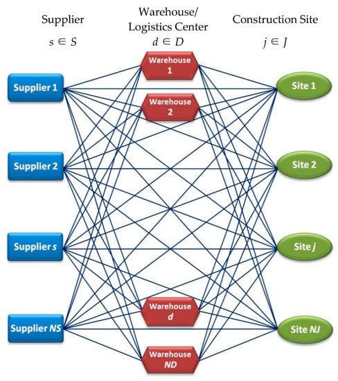
Figure 1.
The proposed CSC Network Structure
The proposed CSC includes three echelons of multiple autonomous facilities:
- Suppliers: suppliers of raw materials, manufacturers (plants), building merchants and manufacturing representatives. They deliver products to project sites directly or indirectly (through echelon 2) from their storage site.
- Warehouses or logistics centers: proprietary or rented storage facilities of subcontractors, referred to as warehouses for simplicity; logistics centers.
- Construction sites: locations to which construction projects are confined, usually with limited storage capacity due to physical constraints.
Both direct and indirect shipments from suppliers to sites are allowed. Echelon 2 may function as a storage buffer and reflects the logistics system used, which may differ across projects and even across time periods of a project. Logistics centers can serve the construction industry by offering high-quality services—storage, transport, assembly, kitting, consolidation, sorting, breaking bulk etc. The benefits of adopting logistics centers in the construction industry have been already discussed [,,,], especially in large construction projects with massive material flows.
In response to the fragmented nature of construction, the model exploits the variety of geographically distributed suppliers seeking appropriate combinations in a long lasting context which encourages strategic alliances, transfer of knowledge, new forms of procurement and investments in communication systems. In this connection, the cost of contractual relationship between supply chain members may also capture costs for workshops, training, robust support for using new technologies or performance warranties. A contractual-base that specifies long employment (continuous or repetitive) over a time horizon encourages joint problem solving, information sharing, effective bargaining and risk-taking.
3.2. Assumptions and Interpretations
- The demand for construction projects over a given time horizon is a deterministic parameter. Hence, the demand of materials per time period is also known according to the project schedule and bill of material.
- The purchase prices of products are known for the overall time horizon (inflation rate is fixed) and discount rates are taken into account for bulk purchase. Cost of purchase is what suppliers charge for their products, taking into account the production cost and any costs involved in the processes of ordering products. No freight transportation costs are included, because these cost items will be studied separately.
- The holding inventory cost in this model is quantity-dependent. Fixed inventory costs are not considered in the optimization context, because they are ascribed to autonomous business entities for their constant operation regardless of which clients and supply chains they serve.
- The echelon of material production is not considered in this context, since the optimal production batches should not derive from the optimization of a CSC driven by a specific construction company; plants are part of several supply chains and serve several clients. However, the output of this model may provide valuable information to suppliers with manufacturing capacity and help them to derive an optimal production plan for their products.
- Safety stock levels are introduced in order to assure a minimum service level at the facilities of echelon 2, which should buffer against demand variations and prevent shortages in any supply chains they serve. The safety stocks usually refer to standardized products and their levels may derive from previous experience, forecasting or other descriptive analysis.
- The transportation cost consists of a fixed cost per shipment between the network nodes and a transportation quantity-dependent variable cost. For the sake of simplicity, we do not consider separate transportation costs for full or less–than–full shipments per order. However, products cannot be transported unless a minimum quantity is met for the transportation modes.
- Material unavailability/shortages are allowed to incur on-site under a known penalty cost, which is proportional to product units. The products that do not meet the demand are backordered and are not considered to be lost sales. We set a limit on the on-site material shortages to cut down the cost component arising from schedule disruption and to avoid any late project delivery.
3.3. Notation
Sets/Indices
| S | Set of suppliers indexed by |
| I | Set of products indexed by |
| J | Set of construction sites indexed by |
| D | Set of warehouses / logistics centers indexed by |
| T | Set of planning time periods indexed by |
Parameters
| Demand of product at site at time period (according to each project’s bill of materials) | |
| Unit purchase cost of product from supplier | |
| Discount rate (%) for bulk purchasing of product from supplier at time period (in quantity greater than a predefined quantity, ) | |
| Variable transportation cost per unit of product shipped from network node to node at time period | |
| Variable transportation cost per unit of product shipped from network node to node at time period | |
| Variable transportation cost per unit of product shipped from network node to node at time period | |
| Fixed transportation cost per shipment from node to node at time period | |
| Fixed transportation cost per shipment from node to node at time period | |
| Fixed transportation cost per shipment from node to node at time period | |
| Maximum distribution capacity of supplier to provide product at time period | |
| Maximum number of units of product that can be shipped on one travel (loading capacity per shipment) from supplier to construction site | |
| Maximum number of units of product that can be shipped on one travel from supplier to warehouse | |
| Maximum number of units of product that can be shipped on one travel from warehouse to construction site | |
| Minimum number of units of product needed to send a shipment from supplier to construction site | |
| Minimum number of units of product needed to send a shipment from supplier to warehouse | |
| Minimum number of units of product needed to send a shipment from warehouse to construction site | |
| Variable inventory cost per unit of product at the storage facility of supplier at time period | |
| Variable inventory cost per unit of product at warehouse at time period | |
| Variable inventory cost per unit of product at construction site at time period | |
| Maximum inventory capacity (in volume) of supplier at any time period | |
| Maximum inventory capacity (in volume) of warehouse at any time period | |
| Maximum inventory capacity (in volume) of construction site at any time period | |
| Inventory space (volume) needed to hold one unit of product | |
| Initial (on-hand) inventory level of product at the storage facility of supplier | |
| Initial (on-hand) inventory level of product at warehouse | |
| Safety inventory level of product at the storage facility of supplier at any time period | |
| Safety inventory level of product at warehouse at any time period | |
| Backorder penalty cost for shortage of one unit of product at construction site | |
| Maximum shortage quantity of product allowed for backordering at construction site at time period without perturbation of the current schedule (expressed as a percentage of the demand ) | |
| Fixed cost related to the establishment of contractual relationship with supplier at time period | |
| Fixed cost related to the establishment of contractual relationship with a contractor holding a warehouse or a logistics provider (indicated by ) at time period | |
| Time period when the construction project at site is completed | |
| M | A very big positive number (infinity value) |
Decision variables
| Quantity of product to be purchased and transported from supplier to warehouse at time period | |
| Quantity of product to be purchased and transported from supplier to construction site at time period | |
| Quantity of product to be transported from warehouse to construction site at time period | |
| Number of shipments of product from supplier to construction site at time period | |
| Number of shipments of product from supplier to warehouse at time period | |
| Number of shipments of product from warehouse to construction site at time period | |
| Inventory level of product at the storage facility of supplier at the end of time period | |
| Inventory level of product at warehouse at the end of time period | |
| Inventory level of product at construction site at the end of time period | |
| Shortage quantity of product backordered at construction site at the end of time period | |
| 1 if supplier is selected at time period ; 0 otherwise | |
| 1 if warehouse is selected at time period ; 0 otherwise | |
| 1 if supplier is selected at time period for delivering product ; 0 otherwise | |
| 1 if warehouse is selected at time period for delivering product ; 0 otherwise | |
| 1 if supplier serves warehouse at time period ; 0 otherwise | |
| 1 if supplier serves site at time period ; 0 otherwise | |
| 1 if warehouse serves site at time period ; 0 otherwise | |
| 1 if supplier provides warehouse with product at time period ; 0 otherwise | |
| 1 if supplier provides site with product at time period ; 0 otherwise | |
| 1 if warehouse provides site with product at time period ; 0 otherwise | |
| 1 if supplier provides all sites with product in a quantity larger than at time period ; 0 otherwise | |
| 1 if supplier provides warehouse with product in a quantity larger than at time period ; 0 otherwise |
3.4. Objective Function
The objective is to minimize the total cost in a supply network that is designed for serving multiple construction projects undertaken by a construction company/general contractor. The cost function includes purchase, transportation, inventory, shortage and contractual relationship cost items, and is subject to Constraints (1)–(48).
3.5. Constraints
3.5.1. Flow Equilibrium Constraints
The set of Constraint (1) indicates that the inventory level of each supplier for every product at the end of each period must be at least equal to the inventory level at the beginning of that period (i.e., at the end of period ) minus the product units transported to the demand market at time interval . The inequality here implies that suppliers may have an incoming flow from a material production echelon (not considered in this optimization context).
Constraint (2) indicate that the inventory level of each warehouse for every product is equal to the previous inventory plus any incoming flow from suppliers and minus any outgoing flow to construction sites at every time period .
Constraint (3) state that the inventory level of product at construction site at the end of period is equal to inventory level at the previous time period plus any incoming flow from suppliers and warehouses, minus the product units utilized/consumed on site. The latter quantity is expressed as the demand for product at time period added to the demand for the backordered quantity at the previous time period minus the shortage occurred at time period .
3.5.2. Constraints on Storage Capacity and Inventory Holding
Constraints (4)–(6) denote that the inventory volume of all products cannot exceed the maximum inventory capacity of each supplier , each warehouse and each construction site at any time period .
Safety stock levels may be established for suppliers and warehouses, as shown in Constraints (7) and (8).
No inventory is allowed at the end of each project () as well as at the end of the planning horizon (), as shown in Constraints (9) and (10).
3.5.3. Constraints on Distribution Capacity and Transportation
The set of Constraint (11) ensures that the quantity of product transported at time period from supplier to the demand market satisfies the upper bound of supplier’s distribution capacity, given that supplier is selected for providing the product at time period , or else the transported quantity is zero.
Constraints (12)–(14) enforce maximum and minimum batch size requirements for each product shipment and thus determine the number of shipments needed at time period to transport a quantity of product from supplier to warehouse , from supplier to site and from warehouse to site , respectively.
3.5.4. Constraints on Quantity Discounts
Bulk discounts are available when buying product from supplier at time period in a quantity larger than . It is important to note that since the general contractor and the subcontractors/logistics-providers are autonomous business entities, the discount shall be applied separately to each quantity ordered by the general contractor for all of their projects and each quantity ordered by each subcontractor/logistics-provider for their warehouse .
The purchase cost items are expressed with the auxiliary variables and which represent the quantities purchased, , in two different cases that cannot hold simultaneously, that is, when the quantities ordered are lesser and greater than , respectively. This means that . Binary variables and big number are used to interpret accordingly these dependencies and force one of the auxiliary variables to zero.
For each quantity ordered by the general contractor for all of their projects (set J)
For each quantity ordered by each subcontractor/logistics-provider for their warehouse :
It is easy to see that Constraints (15)–(22) ensure that the purchasing cost is the quoted purchase price minus the discount only when:
3.5.5. Constraints on Shortage
Constraint (23) set an upper bound for the shortages that may occur at the construction sites, whereas represents that percentage of the total demand that can be backordered without perturbation of the current schedule.
Backlog level at the end of the last time period NT should be zero for fulfilling the total customer demand, as shown in Constraint (24).
The set of Constraint (25) presents the shortage quantity for each product , site and time period as the difference between the total demand of that period (i.e., the sum of the backlog level at and the demand at ) and the product units available on-site (i.e., the sum of inventory and transported product units).
3.5.6. Logical Constraints
Logical constraints are used to achieve consistency between the binary variables and the quantities purchased or transported. In order to link 4-dimensional binary variables with the associated regular variables, fixed-charge Constraints (26)–(31) are used. The rest of the 3- and 2-dimensional binary variables could be interpreted similarly using fixed-charge constraints (see Appendix B), but we choose to use the conditional Constraints (32)–(44) that take advantage of the correlation between variables of higher and lesser dimension and reduce the number of constraints required.
The deployment of all variables from 2-dimentional to 4-dimentional enhances the visibility of the supply chain structure and enables the decision-maker to control of the extent of outsourcing and add further constraints expressing strategic preferences of the construction company, compatibility issues among supply chain partners and logistics-related considerations. To this end, the binary variables can be exploited in various ways within a versatile, flexible and problem-specific managerial decision making tool (see Section 3.6).
3.5.7. General Constraints on Decision Variables
3.6. Introducing Problem-Specific Considerations to the Model
The structure of the proposed model allows the addition of problem-specific constraints expressing specific logistics-related considerations, strategic preferences of the construction company and compatibility issues of supply chain flows. This ability for customized implementation of the model is a novel feature that captures real CSC possibilities and limitations and enhances the applicability, the usefulness and the effectiveness of the model. The following cases show how the binary variables of the model could be exploited for such purposes.
3.6.1. Case I (Material Kitting)
Kitting refers to the combination of several products into a single package unit to be used together on site so that workers will not need extra time to locate and count the needed parts []. The second level of the proposed model may accommodate logistics facilities offering, among others, consolidation and kitting services, which is considered an effective approach to managing the CSC and has drawn interest among researchers [,,].
As an example, let us suppose that products indexed by i = 7, i = 8 and i = 9 are required to be delivered as a kit at the project site indexed by j = 1 at a ratio of 1:2:4 (quantities are expressed in the same units) and that a kitting capability is offered only by a logistics center indexed by d = 2. Then the following constraints should be added in our base model:
(i.e., no direct shipment is allowed from any supplier s to site j = 1 at any time period t for products i = 7, 8, 9)
(i.e., one of the following holds true at any time period t: the logistics center d = 2 ships to site j = 1 either all three products or none of them)
(i.e., the kit shipped to site j = 1 at any time period t includes the three products at a ratio of 1:2:4).
3.6.2. Case II (Strategic Preferences—Single-Supplier Sourcing)
The ability to embed the strategic preferences of the construction company is an advantageous feature of the model. For example, suppose that the construction company may wish to employ at most one supplier per time period for delivering each product. This is translated into the following set of constraints:
In the case of employing not only one supplier (at most) per time period but also the same supplier s for delivering product i, first we add to our base model the binary variable , which equals 1 when supplier is selected for delivering product at one or more time periods over the entire planning horizon and 0 when supplier is not selected at all over the entire planning horizon. Then we add the following conditional constraints to link binary variables with binary variables of higher dimension:
The condition of employing one supplier over the entire time horizon for delivering product i may now be expressed as:
3.6.3. Case III (Strategic Preferences—Multiple-Supplier Sourcing)
The construction company may want to follow a multiple-supplier sourcing strategy for all or for some critical products to reduce supplier dependency and mitigate disruption risks. If each product should be sourced by at least three different suppliers over the entire planning horizon, then the following constraint should be imposed:
3.6.4. Case IV (Compatibility Issues—CSC Products)
The proposed model may include real-life limitations imposed on network configuration and material flows and thus reflect the complex interdependencies among supply chain actors and products. For example, the inclusion of some suppliers may result in exclusion of others due to compatibility of products or business relationships [].
Let us suppose that products indexed by i = 5 and i = 6 are similar to each other prefabricated products designed to be assembled together on-site and that if a supplier is selected for sourcing one of them, then for compatibility reasons the same supplier should source the other product as well. The condition of selecting the same supplier for the two products over the entire time horizon is introduced in the model as follows:
3.6.5. Case V (Compatibility Issues—CSC Actors)
The condition of excluding a network node when a certain node is selected is expressed with mutually exclusive binary variables. For, example, if there are two logistics centers, indexed by d = 1 and d = 2, which cannot serve the same project simultaneously (the same time period), we add the following set of constraints:
4. Computational Experience
4.1. Implementation
The proposed model was implemented in Premium Solver Platform v12.5 by Frontline Solvers, Inc. using the plug-in Gurobi Solver Engine v5.1.0.0 with a free 15-day trial license. Gurobi is a trademark of Gurobi Optimization, Inc. A rich computational experience was obtained based on 133 optimizations. The implementation steps are summarized as follows:
- translating the proposed algebraic model into a spreadsheet model,
- performing numerous zero-tests, tests with extreme input values and other logic tests to see whether the behavior of the model is as expected,
- performing numerous tests with random generated data in order to identify data sets that create a feasible solution space—i.e., satisfy simultaneously all the constraints,
- solving a feasible problem and analyzing the solution,
- conducting sensitivity analysis and multiple parameterized optimizations in order to see the impact of different data on the optimal solution.
4.2. Expected Quality of the Solution
We developed the proposed model as a mixed-integer linear programming (MILP) problem, deliberately avoiding any non-smooth and nonlinear mathematical formulations that could sacrifice the guarantee of optimality and increase the computing time by devising equivalent linear functions with a clever use of binary variables—a good modeling technique suggested by Winston and Albright [] [Appendix A exhibits alternative algebraic formulations of discount-related functions that include (non-linear) products of variables or (non-smooth) functions “IF”—an approach that may be more intuitive to the model developer but eventually was not employed in the proposed model because of its effect on the quality of the solution and the solution time.]. MILP possesses the unique properties of linear models—proportionality, additivity and divisibility—and also offers wide versatile modeling capabilities by means of integer variables [,,].
Generally, the non-continuous solution space of integer programming models makes them non-convex. Finding a globally optimal solution to such a problem is equivalent to solving a global optimization problem and if special methods for global optimization are not used, then only a locally optimal solution could be achieved. Gurobi Solver engine is one of the Frontline’s fastest and most powerful Solvers, especially for MILP problems. It uses advanced primal and dual Simplex and Barrier methods, combined with state-of-the-art Branch and Cut methods and powerful solution heuristics for integer problems, which yield global solutions in record time [].
4.3. Data Generation and Feasibility Implications
Data values were randomly generated using the RANDBETWEEN function of Microsoft Excel—except for the data we entered for zero-tests and the other logic tests. The function produced random values within a range of numbers we specified for each parameter based on rational knowledge. We created a rich unlimited pool of test instances to validate and improve the model structure and offer a well-formulated decision-making tool to researchers and professionals. The numerical examples were manageable and easy to analyze. Hence, obtaining a database from a real-life application to test the model was out of the scope of this paper.
It is acknowledged that imposing as many reasonable constraints as possible tightens the feasible solution space and reduces significantly the solution time in integer programming models, where any algorithm employed must perform an explicit or implicit enumeration of the discrete solution space [,]. Additional constraints (well-founded and non-redundant) are likely to make an integer programming model easier to solve, in contrast with a linear programming model. For example, introducing strategic preferences and other problem-specific constraints to the proposed model (see Section 3.6) may lead to very tight configurations. In that context, a judicious use of data and constraints is required so that the problem would not be so constrained that no candidate solutions are left.
4.4. Model Solution and Analysis
We considered a small-scale network consisting of three products, three time periods, three suppliers, two warehouses/logistics centers and three construction sites (see data in Appendix C). Even this formulation led to a large-scale MILP problem with 1059 variables, 2006 constraints, 1275 bounds and 582 integers, which called for the plug-in large-scale solver engine Gurobi. Premium Solver Platform took less than 5 min to solve this problem instance on a PC with Intel® Core™ i5 CPU 2.67 GHz processor, having 4.00 GB RAM and using 64-bit Windows 7, and found the globally optimal solution Costmin = €108,538.6, which means that there are no other feasible solutions with better objective function values than this.
Figure 2 and Figure 3 show graphical representations of the quantities purchased and transported between network nodes per time period and product, , the quantities stored at each node per time period and product, , the quantities of backorders at each site per time period and product, , and the shipments between network nodes each time period, . Considering space limits, the 0–1 values of variables are omitted, but they are totally in accordance with the meaning of the respective regular variables.
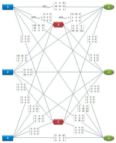
Figure 2.
Quantities purchased and transported between the network nodes.
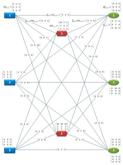
Figure 3.
Inventory levels, shortages and shipments.
The numerical results are plausible and comply with the assumptions and constraints we had intentionally set in order to test the model. Specifically, we considered that not all suppliers provide all of the product types needed for the construction projects (see, for example, Table A5, Table A8, Table A11, Table A28 of Appendix C) and that the projects were initiated at different time periods and were completed at different time periods as well (see Table A1, Table A2 and Table A3 and Table A16 of Appendix C). The results ensure the zero-values we expected for certain variables. Moreover, the results successfully express the logical implications of Section 3.5.4 and Section 3.5.6.
In addition to the optimal solution obtained, the decision maker may also gain valuable insights into the initial problem and diverse instances thereof. Generally, spreadsheet modeling offers unique possibilities for extracting useful business information and creating valuable documentation, but requires well-informed programmers who would not miss such opportunities []. In this model, the decision-maker is able to see whether the constraints expressed as binding (i.e., hold as equalities) or nonbinding (i.e., not met exactly) inequalities and thus identify which of the potential limitations become actual limitations.
For instance, the implementation of the model reveals that Constraint (5) for warehouse and time period is nonbinding:
Likewise, it is proved that for every time period almost 5/6 of the available storage space in warehouse is empty. This information could be disseminated in the supply chain and exploited by the subcontractor/logistic center holding the warehouse. We also observe similar results for the inventory capacity of some construction sites. The decision-maker may then limit the on-site storage facilities in order to remove surplus capabilities and cut down related setup costs.
On the other hand, the left side constraint of (12) for and is binding:
The binding here connotes that the maximum shipment capacity restricts the number of shipments to the lower bound of 5, preventing the objective function from further improvement. If other transportation modes with bigger capacity than 20 units were assigned to this specific trip from to at time period and for product , then a reduced number of shipments would transfer the same product quantity and the value of the objective function would be likely to decrease. Loosening a binding constraint will by no means worsen the objective function, but we need a re-optimization in order to realize the effect.
Thus, the decision maker may focus on the constraints of interest, binding or not, and exploit the information related to the amount of slack or surplus. Various alternative cases could be tested for improving the value of the function by assigning more resources or removing existing resources.
4.5. Sensitivity Analysis
An indispensable part of every modeling process after obtaining the optimal solution should be the sensitivity analysis, especially in those problems where the sensitivity of the optimal solution to input changes is quite unpredictable—e.g., in integer programming problems due to the discontinuity of their solution space. To the best of our knowledge, sensitivity analysis has been neglected for the majority of the CSC optimization models so far. However, sensitivity analysis is a valuable tool that builds the confidence of the decision-maker as it provides the simplest way to cope with moderate uncertainty in parameters, contributes to model validation and refinement, uncovers potential logical errors and identifies which parameters have the highest impact on the optimal solution and thus require precise estimation [,,,,].
In this model, we tackled the issue of sensitivity analysis from two different perspectives, which are seldom reported in practical cases of the modeling literature. Taking advantage of the available tools of Premium Solver Platform, we invoked sensitivity reports and multiple optimization analysis reports. Both types of sensitivity analysis are important, but give answers to different questions. The first addresses the impact of parameter variation on an output formula to which the parameter is algebraically related, without causing changes to the optimal base of the model. The latter traces the impact of parameter variation on any output of the model after the problem has been re-optimized.
All the documentation that was produced in the context of sensitivity analysis (presented in detail in the following sections) indicates a well-conditioned problem and a stable algorithm. This statement comes from the observation that small data changes result in small solution changes. If inputs change slightly and outputs change significantly, we cannot build much confidence in the solutions.
4.5.1. Sensitivity Reports
In the context of sensitivity analysis, the following capabilities of Premium Solver Platform were used:
- Choosing a parameter to serve as a “sensitivity parameter”, defining the desirable range for its variation and invoking the related sensitivity report or graph that shows the effect on the objective function.
- Invoking a “tornado chart” that automatically identifies and displays the first twelve parameters with the highest impact on the selected formula—the cell of total cost. The tornado chart is generated by varying each parameter one at a time by a fixed percentage of its initial value and recording the impact on the selected cell. The tornado chart revealed that the cells with the biggest impact on the total cost are several transportation-related cost parameters, some of the purchase prices as well as some transportation-related variables. Information about the most sensitive variables is useful in exploring how the quantities that the decision-maker can control—in contrast to the problem parameters—affect the total cost. After defining some inputs of highest impact or just of interest to be “sensitivity parameters” with desirable ranges of variation, the tornado chart again ranks the most sensitive parameters, as shown in Figure 4, but now the chart bars indicate the user-determined upper and lower limits, not the percentage changes around the base-case value.
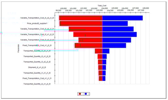 Figure 4. Tornado chart for sensitivity parameters varied within pre-specified ranges.
 - Varying two parameters independently from their lower to upper limits over a pre-specified desirable range and for a pre-specified number of steps and getting documentation of the objective function values in tables or graphs. Such examples are presented in Table 2 and Figure 5. In the interesting case of graphical documentation, we can see the objective function as a surface in 3-dimensional space that illustrates either minor or major impacts of selected parameters and ensures the linearity assumption of the problem. The linear relationships between any parameter and the objective function are shown more explicitly in graphs than in related tables. Graphs also demonstrate easily the relative insensitivity of the objective function to some parameters, such as the unit inventory cost shown in Figure 5b,d.
Table 2. Sensitivity analysis report of varying two parameters independently.
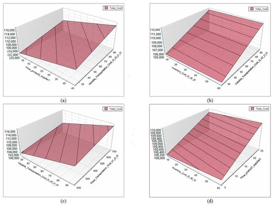 Figure 5. Graphs of the objective value by varying two parameters independently: (a) “Price_i2_s1” and “Var.Transp.Cost_i3_s2_j1_t1”, (b) “Var.Transp.Cost_i3_s2_j1_t1” and “Invent.Cost_i3_d2_t2”, (c) “Var.Transp.Cost_i3_s2_j1_t3” and “Fix.Transp.Cost_s1_j3_t3”, (d) “Invent.Cost_i3_s2_j1_t1” and “Price_i1_s3”.
 - Varying simultaneously several parameters from their lower to upper limits over a pre-specified desirable range and for a pre-specified number of steps and getting documentation of the objective function values in tables. Table 3 shows the resulting values of the objective function for different combinations of the six highest-impact parameters.
Table 3. Sensitivity analysis report for simultaneous variations in the highest-impact parameters.
4.5.2. Multiple Optimization Analysis Report
Performing multiple parameterized optimizations is not explicitly included in sensitivity analysis, since the latter traditionally refers to a fixed optimal basis. Nonetheless, we can think of multiple parameterized optimizations as an extended sensitivity analysis capability that determines the sensitivity of a selected output to input variations by re-optimizing the problem with regard to that input change. Conducting sensitivity analysis with re-optimizations is highly suggested in order to extract the valuable insights one should expect from integer optimization problems [,]. Because of the relatively “irregular” sensitivity of the optimal solution in integer programming models (which arises from the non-continuous solution space), the problem has to be re-solved several times to realize the crucial effect of input variations on the optimal solution.
In a broader context of sensitivity analysis, the following capabilities of Premium Solver Platform were used:
- Choosing a parameter to serve as an “optimization parameter”, defining the desirable range for its variation and invoking a multiple optimization analysis report or graph that shows the effect on the objective function.
- Invoking a “tornado chart” (Figure 6) which displays and ranks the most sensitive inputs with respect to their variation within a user-determined range or an automatic range of percentage changes around the base-case value.
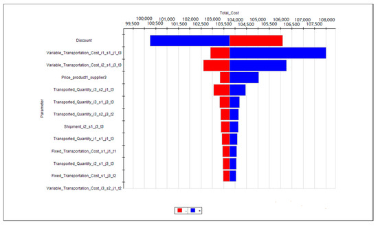 Figure 6. Tornado chart for optimization parameters varied within pre-specified ranges.
 - Varying selected parameters one at a time from their lower to upper limits over a pre-specified desirable range and for a pre-specified number of runs and getting documentation of the objective function values in tables or graphs. Table 4 shows the resulting optimal values of the objective function corresponding to variations of 13 selected parameters one at a time for a number of 5 runs within their variation range (65 runs in total). Similarly, Figure 7 shows the resulting optimal values of the objective function corresponding to variations of 5 selected parameters one at a time for a number of 4 runs within their variation range (20 runs in total). The latter case of graphical representation is very useful in discerning relative sensitivities and particularly the sensitivity and insensitivity ranges of different inputs. For instance, we see that the variation of price does not influence the objective value as much as the variation of demand .
Table 4. Multiple optimization analysis report of varying all selected parameters one at a time (65 runs in total).
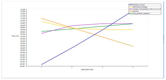 Figure 7. Graphs of the optimal objective value obtained by varying selected parameters one at a time for 4 optimizations (20 runs in total).
 - Varying selected parameters simultaneously, from their lower to upper limits over a pre-specified desirable range and for a user-determined number of runs. The report of Table 5 displays the optimal objective values after 11 optimizations in which we varied 5 selected parameters simultaneously.
Table 5. Multiple optimization analysis report of varying selected parameters simultaneously for 11 runs.
- Varying two parameters independently from their lower to upper limits over a pre-specified desirable range and for a user-determined number of runs. The related documentation may include two-dimensional tabular reports and tree-dimensional charts, as shown in Figure 8. We varied four two-parameter groups for a set of 9 runs (36 runs totally). In the charts we can see the objective function as a surface defined by 9 optimal values obtained from each optimization. Apparently, increasing the number of optimizations required for the generation of each chart results in very well-approximated surfaces. These surfaces readily illustrate the range of parameters where the optimal value of total cost remains unchanged or changes intensely.
 Figure 8. Graphs and related reports of the optimal solution obtained by varying two parameters independently, i.e., (a) “Discount” and “Max_Percent_Shortage”, (b) “Max_Shipm.Capac._i1_s1_j2” and “Var.Transp.Cost_i1_s1_j1_t3”, (c) “Price_i1_s3” and “Demand_i1_j2_t1”, (d) “Discount” and “Demand_i1_j2_t1”, for 9 multiple optimizations (36 runs in total).
To sum up, the reports of multiple parameterized optimizations constitute a straightforward documentation of the objective function value, for which the equivalent manual approach would be very cumbersome. Apart from the objective function, we are also allowed to inspect or monitor any element of the complete solution, e.g., decision variables and binding or non-binding constraints, for each run. Despite the fact that multiple parameterized optimizations reports in integer optimization problems provide more useful insights than a single optimal solution or a sensitivity report, the experience acquired from this model requires us to stress the high computational effort (i.e., time and memory) required for generating the related documentation. This paper encompasses 133 optimizations for solving several instances of the problem.
5. Discussion and Concluding Remarks
This paper presented an innovative dynamic mixed-integer linear programming model for an integrated contractor-led three-echelon CSC which addresses network design and material flow issues and aims to minimize the costs accumulated across multiple supply chains serving the projects undertaken by a general contractor/construction company over a time horizon. Decisions on “how much to buy?”, “when to buy?”, “from which supplier or subcontractor/logistics provider?”, “where to deliver?”, “where to store and for how long?”, “which product from whom?”, “when to replenish a warehouse?”, “what deficit to be incurred on-site?”, etc. are addressed. Decisions are made at each period along the considered time horizon developing a challenging strategic planning environment and can be updated if the schedule is subject to change. Therefore, the model allows a dynamic tracking of projects and also a financial evaluation of each period’s decisions (cash flows), which could not be possible if the time in the model was considered in a continuous mode.
Before taking decisions for a real-life problem, model implementation provides artificial feedback cycles (“what if?” analysis) for a wide range of assumptions, enabling the decision maker to negotiate with supply chain partners based on information that was not previously quantifiable. This analysis also identifies the most significant inputs for achieving the desired outcome, reveals the importance of each numerical assumption and shows which parameters require rough or precise estimates. After taking decisions for a real-life problem based on the model implementation, full access to optimal purchase–inventory–distribution plans for the entire time horizon may be available to all selected suppliers, subcontractors and logistics centers so as to optimize the CSC information flow and allow suppliers with production capacities to make in turn optimal production decisions.
The novelty of this model lies in merging temporal and project-based supply chains into a sustainable dynamic supply chain network with repetitive flows, large scope contracts, strategic alliances and economies of scale, and in allowing customized applications of the network design and material flow optimization problem under any logistics system. A distinctive feature of the model is that it yields the optimal network design, the optimal material quantities to be purchased and transported, the optimal number of shipments and the optimal inventory levels in three echelons of a dynamic CSC allowing direct and indirect transportation of materials from suppliers to construction sites, discounts for bulk purchases and incorporation of strategic preferences.
The model is general enough to be implemented by any business entity or individual with the appropriate leverage power to act as a system integrator for the entire supply network established for the needs of multiple projects but also allows some customization; it may be specific enough to include strategic preferences controlling the extent of outsourcing, compatibility issues between products and supply chain partners or logistics-related considerations such as material consolidation. All these features make this model a versatile and flexible managerial decision making tool.
Considering the fact that optimization depends not only on efficient and robust algorithms but also on good modeling techniques, careful interpretation of results and user-friendly software [], we followed acknowledged principles of spreadsheet modeling and post-solution analysis [,,,,]. This corresponds to a continuous effort for improving the conceptualization and formulation of the model, and using the model as a tool for gaining real insights into the problem. Translating the proposed model from its algebraic form into a spreadsheet model was proved to be an extremely useful process: the algebraic formulation was improved with regard to the expected optimization methods and many insights and limitations were revealed. For any problem, there may exist many alternative mathematical formulations but the main concern is to create a formulation that is as better as possible in terms of solution time and reliability.
The formulation of the model as a mixed-integer linear programming model provided broad modeling capabilities—broader than the capabilities that linear programming models offer []. In this paper, we showed how to use binary variables in a model formulation to: (a) represent yes/no decisions, if/then statements, mutual exclusivity and other conditional restrictions based on strategic preferences; (b) avoid some sort of nonlinearity (product terms) in the objective function and the constraints; and (c) model fixed costs in the objective function. Admittedly, sensitivity analysis for MILP models is much more crucial compared with linear programming [], because input variations in integer problems may result in rather erratic changes of the optimal solution and thus it pays more to obtain the revised optimal solution. In light of this, we conducted sensitivity analysis and multiple parameterized optimizations to address that crucial effect—re-optimizations are highly recommended for these types of problems [,,].
Validation efforts on the proposed model included numerous tests with zero or extreme values that yielded the results expected, sensitivity analysis, multiple parameterized optimizations and implementation of alternative equivalent structures for some parts of the algebraic model. Post-solution analysis of different data instances revealed a well-conditioned model. According to McCarl and Spreen, validating predictive models may involve comparison of the model predictions with real world results, whereas for prescriptive models “decision maker reliance is the ultimate validation test” [], which is the case of optimization models.
A possible limitation of this model is that its formulation may lead to large-scale MILP problems that require considerable computational effort, especially in real-life applications. This complexity stems from the model including several—not superfluous—constraints with multi-dimensional variables to realistically represent real-life problems, reduce the abstraction and provide possibilities for customization. In favor of computational effort, the decision maker may loosen a constrained problem or prioritize the elements to be included for optimization. In fact, many times the optimization focus is only on a few critical products or suppliers. Moreover, computer technology and solver engines are undergoing tremendous advances that hopefully will allow coping with large-scale real-life problems with acceptable time and memory complexity.
6. Further Research
Future trends in CSC modeling include multi-objective optimization models that integrate and consider simultaneously many and even conflicting goals (e.g., cost, service level, time, responsiveness, profit), and stochastic models for the consideration of uncertainty which is inherently tied to the construction industry’s nature. Another research direction concerns the modeling of global construction supply chains aiming at the profit maximization with the inclusion of exchange rates, taxes, tariffs and duty drawbacks. Moreover, green logistics (e.g., flow of construction and demolition waste from sites to recycling centers or management of fleet and transportation channels with respect to CO2 emissions and fuel consumption) and reverse logistics (e.g., flow of non-consumable and no longer required resources at the construction sites back to warehouses) could be considered in model formulations. It is highly recommended to take advantage of the vehicles classification system according to the environmental impact of their engine, as defined by governmental specifications, and select the appropriate combination of routes and modes through the optimization process.
An extension of this model may include shipments between sites along with direct and indirect shipments from suppliers to construction sites. If some of the construction sites are close to each other, the products shipped to one site may be combined with the products required in the other projects in order to save on shipping cost. This is an opportunity for suppliers to apply inter/intraproject SCM and create a win-win situation [] and may be included in the proposed model with additional variables, parameters and constraints. Another extension is to focus on the transportation problem at the operational level by adding to the transportation cost additional indexes (higher than fourth dimension) which stand for the mode of transport, the transportation capacity level and/or the transportation channel to be selected among many available. Finally, a promising future work based on the present model includes the connection to project’s activities and the consideration of lead times in a continuous time mode. Thus, we could study the impact of materials shortages on critical activities and, consequently, on the project’s delivery date.
Author Contributions
A.K.: Conceptualization, Data curation, Investigation, Software, Visualization, Writing—original draft. S.K.: Project administration, Supervision, Methodology, Validation, Writing—review & editing. All authors have read and agreed to the published version of the manuscript.
Funding
This research received no external funding.
Conflicts of Interest
The authors declare no conflict of interest.
Appendix A
In this section, we present some alternatives for the consideration of discounts in the model.
1st alternative: Introducing IF functions in the definition of the purchase price:
Using an IF function in the purchase cost formula of the spreadsheet model results in a non-smooth optimization problem. Premium Solver Platform provides a non-smooth model transformation option (preprocessing technique), which tries to eliminate the discontinuous and/or non-differentiable functions by replacing them with additional variables constraints that have the same effect on the model. However, the implementation of the model revealed that this automatic transformation was not sufficient to make the overall model linear. The other option was to employ solvers with multi-start or metaheuristic techniques—which might yield acceptable results, though the guarantee of optimality would be completely sacrificed and the computing time would be considerably long.
2nd alternative: Introducing binary variables in the definition of the purchase price for the quantities ordered by each independent business entity and adding fixed-charge constraints:
For the quantities ordered by the construction company for all the projects:
For the quantities ordered by each business entity of echelon 2:
Here the purchase price is transformed from a fixed value into a linear function that depends on the quantities ordered. The fact that the purchase price is multiplied with another variable in the objective function results in a quadratic programming problem, a simple form of non-linear programming. Dealing with integer non-linear problems, we shall employ global methods or multi-start local methods (included in solvers) that will try to find the best among many local optima. The result is to either compromise with a locally optimal solution or seek a near-optimal solution along with possibly long computing times and severe limits on the size of problems that are solved to global optimality.
3rd alternative: Dividing the quantities ordered into auxiliary variables, introducing binary variables in their definition and adding fixed-charge constraints:
For the quantities ordered by the construction company for all the projects:
For the quantities ordered by each business entity of echelon 2:
Likewise, the 3rd alternative also results in a quadratic programming problem with the above-mentioned results, since the quantities include multiplications of two other variables. In the objective function, the purchase price is now multiplied with the quantity ordered in two different and non-simultaneous cases:
Appendix B
For each binary variable, two sets of fixed-charge/linking constraints are introduced (see right and left column) without exploiting the correlation among binary variables of different dimension—an approach which suggests “reinventing the wheel” but is equivalent to that of Section 3.5.4 and results in the desired logical consistency.
Appendix C
Table A1.
Demand at period 1 (units).
Table A1.
Demand at period 1 (units).
| i = 1 | i = 2 | i = 3 | |
| j = 1 | 55 | 48 | 90 |
| j = 2 | 100 | 18 | 50 |
| j = 3 | 0 | 0 | 0 |
Table A2.
Demand at period 2 (units).
Table A2.
Demand at period 2 (units).
| i = 1 | i = 2 | i = 3 | |
| j = 1 | 90 | 32 | 56 |
| j = 2 | 102 | 25 | 0 |
| j = 3 | 35 | 41 | 135 |
Table A3.
Demand at period 3 (units).
Table A3.
Demand at period 3 (units).
| i = 1 | i = 2 | i = 3 | |
| j = 1 | 85 | 32 | 105 |
| j = 2 | 0 | 0 | 0 |
| j = 3 | 50 | 60 | 82 |
Table A4.
Percentage (%) of demand expressing the maximum shortage allowed (considered here the same for any time period).
Table A4.
Percentage (%) of demand expressing the maximum shortage allowed (considered here the same for any time period).
| i = 1 | i = 2 | i = 3 | |
| j = 1 | 0.2 | 0.2 | 0.2 |
| j = 2 | 0.2 | 0.2 | 0.2 |
| j = 3 | 0.2 | 0.2 | 0.2 |
Table A5.
Unit purchase cost (€).
Table A5.
Unit purchase cost (€).
| i = 1 | i = 2 | i = 3 | |
| s = 1 | 9 | 30 | 4.5 |
| s = 2 | 8.5 | – | 5 |
| s = 3 | 10 | 32 | – |
Table A6.
Discount rate at any time period t (considered here the same for any time period).
Table A6.
Discount rate at any time period t (considered here the same for any time period).
| i = 1 | i = 2 | i = 3 | |
| s = 1 | 0.2 | 0.2 | 0.2 |
| s = 2 | 0.2 | – | 0.2 |
| s = 3 | 0.2 | 0.2 | – |
Table A7.
Variable transportation cost per unit of product 1 (€) (considered here the same for any t).
Table A7.
Variable transportation cost per unit of product 1 (€) (considered here the same for any t).
| j = 1 | j = 2 | j = 3 | d = 1 | d = 2 | |
| s = 1 | 40 | 20 | 60 | 25 | 71 |
| s = 2 | 72 | 67 | 78 | 30 | 45 |
| s = 3 | 59 | 95 | 24 | 45 | 35 |
| d = 1 | 20 | 36 | 36 | – | – |
| d = 2 | 29 | 43 | 34 | – | – |
Table A8.
Variable transportation cost per unit of product 2 (€) (considered here the same for any t).
Table A8.
Variable transportation cost per unit of product 2 (€) (considered here the same for any t).
| j = 1 | j = 2 | j = 3 | d = 1 | d = 2 | |
| s = 1 | 38 | 89 | 49 | 83 | 47 |
| s = 2 | – | – | – | – | – |
| s = 3 | 79 | 45 | 95 | 47 | 45 |
| d = 1 | 50 | 53 | 48 | – | – |
| d = 2 | 95 | 48 | 43 | – | – |
Table A9.
Variable transportation cost per unit of product 3 (€) (considered here the same for any t).
Table A9.
Variable transportation cost per unit of product 3 (€) (considered here the same for any t).
| j = 1 | j = 2 | j = 3 | d = 1 | d = 2 | |
| s = 1 | 98 | 69 | 54 | 82 | 25 |
| s = 2 | 61 | 48 | 47 | 32 | 79 |
| s = 3 | – | – | – | – | – |
| d = 1 | 44 | 63 | 45 | – | – |
| d = 2 | 97 | 61 | 37 | – | – |
Table A10.
Fixed transportation cost (€) (considered here the same for any t).
Table A10.
Fixed transportation cost (€) (considered here the same for any t).
| j = 1 | j = 2 | j = 3 | d = 1 | d = 2 | |
| s = 1 | 447 | 289 | 467 | 340 | 419 |
| s = 2 | 654 | 698 | 520 | 536 | 598 |
| s = 3 | 600 | 490 | 267 | 498 | 340 |
| d = 1 | 300 | 329 | 400 | – | – |
| d = 2 | 780 | 290 | 679 | – | – |
Table A11.
Maximum distribution capacity at time period 1 (units).
Table A11.
Maximum distribution capacity at time period 1 (units).
| i = 1 | i = 2 | i = 3 | |
| s = 1 | 100 | 78 | 100 |
| s = 2 | 98 | – | 130 |
| s = 3 | 68 | 100 | – |
Table A12.
Maximum distribution capacity at time period 2 (units).
Table A12.
Maximum distribution capacity at time period 2 (units).
| i = 1 | i = 2 | i = 3 | |
| s = 1 | 100 | 78 | 123 |
| s = 2 | 98 | – | 130 |
| s = 3 | 68 | 100 | – |
Table A13.
Maximum distribution capacity at time period 3 (units).
Table A13.
Maximum distribution capacity at time period 3 (units).
| i = 1 | i = 2 | i = 3 | |
| s = 1 | 100 | 78 | 200 |
| s = 2 | 98 | – | 130 |
| s = 3 | 100 | 100 | – |
Table A14.
Unit backorder penalty cost (€) (considered here the same for any t).
Table A14.
Unit backorder penalty cost (€) (considered here the same for any t).
| i = 1 | i = 2 | i = 3 | |
| j = 1 | 30 | 60 | 25 |
| j = 2 | 25 | 50 | 20 |
| j = 3 | 25 | 50 | 20 |
Table A15.
Inventory space per unit of product (m3).
Table A15.
Inventory space per unit of product (m3).
| i = 1 | 3 |
| i = 2 | 2 |
| i = 3 | 1.5 |
Table A16.
Time period of project beginning and completion.
Table A16.
Time period of project beginning and completion.
| Start | ||
|---|---|---|
| Project 1 | t = 1 | t = 3 |
| Project 2 | t = 1 | t = 2 |
| Project 3 | t = 2 | t = 3 |
Table A17.
Maximum loading capacity per shipment of product 1 (units).
Table A17.
Maximum loading capacity per shipment of product 1 (units).
| j = 1 | j = 2 | j = 3 | d = 1 | d = 2 | |
| s = 1 | 40 | 20 | 20 | 30 | 40 |
| s = 2 | 25 | 25 | 20 | 50 | 50 |
| s = 3 | 25 | 25 | 25 | 45 | 50 |
| d = 1 | 34 | 34 | 45 | – | – |
| d = 2 | 40 | 27 | 40 | – | – |
Table A18.
Minimum loading capacity per shipment of product 1 (units).
Table A18.
Minimum loading capacity per shipment of product 1 (units).
| j = 1 | j = 2 | j = 3 | d = 1 | d = 2 | |
| s = 1 | 20 | 10 | 12 | 15 | 10 |
| s = 2 | 15 | 10 | 12 | 15 | 15 |
| s = 3 | 12 | 10 | 10 | 13 | 20 |
| d = 1 | 10 | 10 | 15 | – | – |
| d = 2 | 15 | 10 | 10 | – | – |
Table A19.
Maximum loading capacity per shipment of product 2 (units).
Table A19.
Maximum loading capacity per shipment of product 2 (units).
| j = 1 | j = 2 | j = 3 | d = 1 | d = 2 | |
| s = 1 | 10 | 10 | 8 | 14 | 10 |
| s = 2 | 1 | 1 | 1 | 1 | 1 1 |
| s = 3 | 12 | 10 | 10 | 10 | 12 |
| d = 1 | 15 | 20 | 20 | – | – |
| d = 2 | 10 | 12 | 12 | – | – |
1 We do not assign zero values to these loading capacities, although supplier s = 2 does not provide any product i = 2 and supplier s = 3 does not provide any product i = 3, because these quantities are used as denominators in Constraints (12)–(14).
Table A20.
Minimum loading capacity per shipment of product 2 (units).
Table A20.
Minimum loading capacity per shipment of product 2 (units).
| j = 1 | j = 2 | j = 3 | d = 1 | d = 2 | |
| s = 1 | 4 | 4 | 4 | 4 | 4 |
| s = 2 | 1 | 1 | 1 | 1 | 1 1 |
| s = 3 | 6 | 6 | 8 | 4 | 4 |
| d = 1 | 5 | 8 | 8 | – | – |
| d = 2 | 5 | 8 | 8 | – | – |
1 We do not assign zero values to these loading capacities, although supplier s = 2 does not provide any product i = 2 and supplier s = 3 does not provide any product i = 3, because these quantities are used as denominators in Constraints (12)–(14).
Table A21.
Maximum loading capacity per shipment of product 3 (units).
Table A21.
Maximum loading capacity per shipment of product 3 (units).
| j = 1 | j = 2 | j = 3 | d = 1 | d = 2 | |
| s = 1 | 50 | 45 | 50 | 25 | 25 |
| s = 2 | 45 | 50 | 50 | 30 | 35 |
| s = 3 | 1 | 1 | 1 | 1 | 1 1 |
| d = 1 | 50 | 40 | 40 | – | – |
| d = 2 | 35 | 48 | 50 | – | – |
1 We do not assign zero values to these loading capacities, although supplier s = 2 does not provide any product i = 2 and supplier s = 3 does not provide any product i = 3, because these quantities are used as denominators in Constraints (12)–(14).
Table A22.
Minimum loading capacity per shipment of product 3 (units).
Table A22.
Minimum loading capacity per shipment of product 3 (units).
| j = 1 | j = 2 | j = 3 | d = 1 | d = 2 | |
| s = 1 | 10 | 12 | 10 | 12 | 12 |
| s = 2 | 10 | 10 | 8 | 10 | 10 |
| s = 3 | 1 | 1 | 1 | 1 | 1 1 |
| d = 1 | 20 | 16 | 16 | – | – |
| d = 2 | 15 | 15 | 20 | – | – |
1 We do not assign zero values to these loading capacities, although supplier s = 2 does not provide any product i = 2 and supplier s = 3 does not provide any product i = 3, because these quantities are used as denominators in Constraints (12)–(14).
Table A23.
Unit variable inventory cost (€) (considered here the same for any time period).
Table A23.
Unit variable inventory cost (€) (considered here the same for any time period).
| i = 1 | i = 2 | i = 3 | |
| s = 1 | 24 | 10 | 19 |
| s = 2 | 23 | – | 25 |
| s = 3 | 17 | 20 | – |
| d = 1 | 2 | 11 | 5 |
| d = 2 | 9 | 8 | 32 |
| j = 1 | 14 | 15 | 10 |
| j = 2 | 10 | 26 | 30 |
| j = 3 | 7 | 15 | 17 |
Table A24.
Maximum inventory capacity (m3).
Table A24.
Maximum inventory capacity (m3).
| s = 1 | 800 |
| s = 2 | 290 |
| s = 3 | 550 |
| d = 1 | 600 |
| d = 2 | 943 |
| j = 1 | 167 |
| j = 2 | 325 |
| j = 3 | 300 |
Table A25.
Initial inventory level (units).
Table A25.
Initial inventory level (units).
| i = 1 | i = 2 | i = 3 | |
| s = 1 | 6 | 2 | 6 |
| s = 2 | 5 | – | 5 |
| s = 3 | 9 | 2 | – |
| d = 1 | 5 | 2 | 5 |
| d = 2 | 10 | 5 | 5 |
Table A26.
Safety inventory level (units).
Table A26.
Safety inventory level (units).
| i = 1 | i = 2 | i = 3 | |
| s = 1 | 5 | 2 | 5 |
| s = 2 | 5 | – | 5 |
| s = 3 | 4 | 2 | – |
| d = 1 | 5 | 2 | 5 |
| d = 2 | 3 | 4 | 3 |
Table A27.
Contractual relationship cost (€) (considered here the same for any time period).
Table A27.
Contractual relationship cost (€) (considered here the same for any time period).
| s = 1 | 435 |
| s = 2 | 500 |
| s = 3 | 450 |
| d = 1 | 267 |
| d = 2 | 400 |
Table A28.
Minimum quantity for purchase discounts (units) (considered here the same for any time period).
Table A28.
Minimum quantity for purchase discounts (units) (considered here the same for any time period).
| i = 1 | i = 2 | i = 3 | |
| s = 1 | 50 | 30 | 40 |
| s = 2 | 60 | – | 45 |
| s = 3 | 70 | 40 | – |
References
- Xue, X.; Sun, C.; Wang, Y.; Shen, Q. A Two-Level Programming Method for Collaborative Scheduling in Construction Supply Chain Management. In Cooperative Design, Visualization, and Engineering; CDVE 2007; Lecture Notes in Computer Science; Luo, Y., Ed.; Springer: Berlin/Heidelberg, Germany, 2007; Volume 4674, pp. 290–297. [Google Scholar] [CrossRef]
- Khalfan, M.M.A.; Maqsood, T. Supply chain capital in construction industry: Coining the term. Int. J. Manag. Proj. Bus. 2012, 5, 300–310. [Google Scholar] [CrossRef]
- De Souza, D.V.S.; Koskela, L. On Improvement in Construction Supply Chain Management. In Proceedings of the 20th Annual Conference of the International Group for Lean Construction, San Diego, CA, USA, 18–20 July 2012. [Google Scholar]
- Love, P.E.D.; Irani, Z.; Edwards, D.J. A seamless supply chain management model for construction. Supply Chain Manag. 2004, 9, 43–56. [Google Scholar] [CrossRef]
- Xue, X.; Li, X.; Shen, Q.; Wang, Y. An agent-based framework for supply chain coordination in construction. Autom. Constr. 2005, 14, 413–430. [Google Scholar] [CrossRef]
- Hai, T.; Md Yusof, A.; Ismail, S.; Wei, L. A Conceptual Study of Key Barriers in Construction Project Coordination. J. Organ. Manag. Stud. 2012, 1–14. [Google Scholar] [CrossRef]
- Koskela, L. Application of the New Production Philosophy to Construction; CIFE Technical Report n. 72; Stanford University: Stanford, CA, USA, 1992. [Google Scholar]
- Ballard, G.; Howell, G. What Kind of Production is Construction? In Proceedings of the 6th Conference of the International Group for Lean Construction, Guaruja, Brazil, 13–15 August 1998. [Google Scholar]
- O’Brien, W.J.; London, K.; Vrijhoef, R. Construction supply chain modeling: A research review and interdisciplinary research agenda. In Proceedings of the 10th Annual Conference of the International Group for Lean Construction, Gramado, Brazil, 6–8 August 2002; pp. 1–19. [Google Scholar]
- Keramati, A. Supply chain integration: A modelling classification. In Proceedings of the Eighth Annual International Symposium on Supply Chain Management, Toronto, ON, Canada, 26–28 September 2010. [Google Scholar]
- Shapiro, J.F. Modeling the Supply Chain, 2nd ed.; Cengage Learning: Boston, MA, USA, 2007; p. 624. [Google Scholar]
- Chen, D.-S.; Batson, R.G.; Dang, Y. Applied Integer Programming: Modeling and Solution; John Wiley & Sons, Inc.: Hoboken, NJ, USA, 2010; p. 488. [Google Scholar] [CrossRef]
- Bankvall, L.; Bygballe, L.E.; Dubois, A.; Jahre, M. Interdependence in supply chains and projects in construction. Supply Chain Manag. 2010, 15, 385–393. [Google Scholar] [CrossRef]
- Koutsokosta, A.; Katsavounis, S. Review of the Model-Based Supply Chain Management Research in the Construction Industry. Int. J. Ind. Manuf. Eng. 2015, 9, 2318–2324. [Google Scholar] [CrossRef]
- O’Brien, W.J.; Formoso, C.T.; Vrijhoef, R.; London, K.A. Construction Supply Chain Management Handbook; CRC Press: Boca Raton, FL, USA, 2008; p. 520. [Google Scholar] [CrossRef]
- Pryke, S. (Ed.) Construction Supply Chain Management: Concepts and Case Studies; Wiley-Blackwell: Oxford, UK, 2009; p. 245. [Google Scholar] [CrossRef]
- Koçtaş, Ö.; Tek, Ö.B. Construction Supply Chains: A proposal to develop a new conceptual model. In Proceedings of the International Logistics and Supply Chain Congress, Cappadocia, Kayseri, Turkey, 7–9 November 2013. [Google Scholar]
- Nocedal, J.; Wright, S.J. Numerical Optimization, 2nd ed.; Springer Science and Business Media: New York, NY, USA, 2006; p. 686. [Google Scholar] [CrossRef]
- Winston, W.L.; Albright, S.C. Practical Management Science, 6th ed.; Cengage Learning: Boston, MA, USA, 2019; p. 888. [Google Scholar]
- Baker, K.R. Optimization Modeling with Spreadsheets, 3rd ed.; John Wiley & Sons: Hoboken, NJ, USA, 2016; p. 400. [Google Scholar]
- Jian-hua, C.; Wan, T. Time-cost trade-off problem in construction supply chain: A bi-level programming decision model. In Proceedings of the 2010 International Conference on Management Science and Engineering, 17th Annual Conference Proceedings, Melbourne, VIC, Australia, 24–26 November 2010; pp. 212–217. [Google Scholar] [CrossRef]
- Pan, N.-H.; Lee, M.-L.; Chen, S.-Q. Construction Material Supply Chain Process Analysis and Optimization. J. Civ. Eng. Manag. 2011, 17, 357–370. [Google Scholar] [CrossRef]
- Xu, X.; Zhao, Y.; Chen, C.-Y. Project-driven supply chains: Integrating safety-stock and crashing decisions for recurrent projects. Ann. Oper. Res. 2012, 241. [Google Scholar] [CrossRef]
- Xu, J.; Wei, P. Production-distribution planning of construction supply chain management under fuzzy random environment for large-scale construction projects. J. Ind. Manag. Optim. 2013, 9, 31–56. [Google Scholar] [CrossRef]
- Said, H.; El-Rayes, K. Automated multi-objective construction logistics optimization system. Autom. Constr. 2014, 43, 110–122. [Google Scholar] [CrossRef]
- Hsu, P.-Y.; Angeloudis, P.; Aurisicchio, M. Optimal logistics planning for modular construction using two-stage stochastic programming. Autom. Constr. 2018, 94, 47–61. [Google Scholar] [CrossRef]
- Feng, C.; Ma, Y.; Zhou, G.; Ni, T. Stackelberg Game Optimization for Integrated Production-Distribution-Construction System in Construction Supply Chain. Knowl. Based Syst. 2018, 157, 52–67. [Google Scholar] [CrossRef]
- Golpîra, H. Optimal Integration of the Facility Location Problem into the Multi-Project Multi-Supplier Multi-Resource Construction Supply Chain Network Design under the Vendor Managed Inventory Strategy. Expert Syst. Appl. 2019, 139. [Google Scholar] [CrossRef]
- Sobotka, A.; Czarnigowska, A.; Stefaniak, K. Logistics of construction projects. Found. Civ. Environ. Eng. 2005, 6, 203–216. [Google Scholar]
- Fengyu, Q.; Shengyue, H. The Research on the Application of Supply Chain Management in Construction. In Proceedings of the 13th International Conference on Management Science and Engineering, Lille, France, 5–7 October 2006; pp. 1191–1196. [Google Scholar]
- Hamzeh, F.R.; Tommelein, I.D.; Ballard, G.; Kaminsky, P.M. Logistics Centers to Support Project-based Production in the Construction Industry. In Proceedings of the 15th Annual Conference of the International Group for Lean Construction, East Lansing, MI, USA, 18–20 July 2007; pp. 170–180. [Google Scholar]
- Dakhli, Z.; Lafhaj, Z. Considering Materials Management in Construction: An Exploratory Study. Logistics 2018, 2, 7. [Google Scholar] [CrossRef]
- Guerlain, C.; Renault, S.; Ferrero, F. Understanding Construction Logistics in Urban Areas and Lowering Its Environmental Impact: A Focus on Construction Consolidation Centres. Sustainability 2019, 11, 6118. [Google Scholar] [CrossRef]
- Arashpour, M.; Bai, Y.; Aranda-Mena, G.; Bab-Hadiashar, A.; Hosseini, M.R.; Kalutara, P. Optimizing decisions in advanced manufacturing of prefabricated products: Theorizing supply chain configurations in off-site construction. Autom. Constr. 2017, 84, 146–153. [Google Scholar] [CrossRef]
- Powell, S.G.; Baker, K.R. Management Science: The Art of Modeling with Spreadsheets, 5th ed.; John Wiley & Sons: Hoboken, NJ, USA, 2017. [Google Scholar]
- Frontline Systems, Inc. Frontline Solvers: User Guide, version 12.5; Frontline Systems, Inc.: Incline Village, NV, USA, 2013. [Google Scholar]
- Bradley, S.P.; Hax, A.C.; Magnanti, T.L. Applied Mathematical Programming; Addison-Wesley Publishing Company: Boston, MA, USA, 1977. [Google Scholar]
- Powell, S.G.; Batt, R.J. Spreadsheet Modeling for Insight. In Proceedings of the International Workshop on the Foundations of Spreadsheets, Rome, Italy, 30 September 2004; Elsevier Science B.V.: Amsterdam, The Netherlands, 2008. [Google Scholar]
- Lawrence, J.A.; Pasternack, B.A. Applied Management Science: Modeling, Spreadsheet Analysis, and Communication for Decision Making, 2nd ed.; John Wiley & Sons: New York, NY, USA, 2002; p. 768. [Google Scholar]
- Anderson, D.R.; Sweeney, D.J.; Williams, T.A.; Camm, J.D.; Cochran, J.J.; Fry, M.J.; Ohlmann, J.W. An Introduction to Management Science: Quantitative Approaches to Decision Making, 15th ed.; Cengage Learning: Boston, MA, USA, 2016; p. 912. [Google Scholar]
- Ragsdale, C. Spreadsheet Modeling and Decision Analysis: A Practical Introduction to Management Science, 8th ed.; Cengage Learning: Mason, OH, USA, 2018; p. 864. [Google Scholar]
- Geoffrion, A.M. A guided tour of recent practical advances in integer linear programming. Omega 1976, 4, 49–57. [Google Scholar] [CrossRef]
- McCarl, B.A.; Spreen, T.H. Applied Mathematical Programming Using Algebraic Systems; Texas A&M University: College Station, TX, USA, 2011; p. 567. [Google Scholar]
© 2020 by the authors. Licensee MDPI, Basel, Switzerland. This article is an open access article distributed under the terms and conditions of the Creative Commons Attribution (CC BY) license (http://creativecommons.org/licenses/by/4.0/).