Abstract
Background: This study addresses optimising fleet size in a system with a heterogeneous truck fleet, aiming to minimise transportation costs in interfacility material transfer operations. Methods: The material transfer process is modelled using a closed queueing network (CQN) that considers heterogeneous nodes and customised service times tailored to the unique characteristics of various truck types and their transported materials. The optimisation problem is formulated as a mixed-integer nonlinear programming (MINLP), falling into the NP-Hard, making exact solution computation challenging. A numerical approximation method, a modified sequential quadratic programming (SQP) method coupled with a mean value analysis (MVA) algorithm, is employed to overcome this challenge. Validation is conducted using a discrete event simulation (DES) model. Results: The proposed analytical model tested within a steel manufacturing plant’s material transfer process. The results showed that the analytical model achieved comparable optimisation of the heterogeneous truck fleet size with significantly reduced response times compared to the simulation method. Furthermore, evaluating performance metrics, encompassing response time, utilisation rate, and cycle time, revealed minimal discrepancies between the analytical and the simulation results, approximately ±8%, ±8%, and ±7%, respectively. Conclusions: These findings affirm the presented analytical approach’s robustness in optimising interfacility material transfer operations with heterogeneous truck fleets, demonstrating real-world applications.
1. Introduction
Modern-day supply chains are undergoing an inevitable surge in complexity, marked by the involvement of numerous entities. The escalating expectations of customers, stringent lead time requirements, demands for customisation, and the imperative of sustainability measures have prompted organisations to concentrate on the comprehensive optimisation of their operational processes. In response to the dynamic shifts in customer demands, manufacturing and service organisations must transition from conventional “one size fits all” business models to more nuanced “markets of one” paradigms. Consequently, these transformative alterations within supply chain ecosystems present formidable challenges in effectively managing logistics operations for organisations across manufacturing and service sectors.
In the broad landscape of logistics operations, three principal categories can be discerned: inbound, outbound, and intra-logistics. The latter has recently garnered increased scholarly and practical attention within process-based industries [1]. Moreover, emphasising the significance of intra-logistics functions, extant research indicates that the absence of a well-structured intra-logistics system may precipitate supply disruptions, machine idling, and prevalent inefficiency within the overall operational system [2,3,4,5,6]. This underscores the critical role played by intra-logistics operations in sustaining the seamless flow of materials and information, particularly within dynamic and complex supply chain environments.
Material handling is a pivotal logistics function that ensures the unbroken continuum of operations by incorporating the principles of “time and place utility” within its procedural framework. The evolutionary trajectory of material handling systems (MHS), propelled by integrating smart manufacturing and digitalisation concepts, strives towards realising predefined objectives while minimising the necessity for human intervention and oversight [7]. In modern MHS frameworks, there is a discernible trend towards incorporating advanced technologies such as autonomous mobile robots (AMR), automated guided vehicles (AGV), and drones. These technological advancements are progressively harnessed to augment material handling processes’ overall efficiency and effectiveness. Even with the strides made in automation, conventional trucks persist in their role within specific material handling activities, notably in contexts such as transportation within mining pits, agricultural fields, and dry-bulk cargo terminals.
The complexity of decision making within material handling equipment (MHE) is illustrated in Figure 1, which delineates a decision tree based on load types and features [8]. This systematic representation is a visual aid for navigating the nuanced landscape of material handling, facilitating informed choices aligned with specific operational requirements.
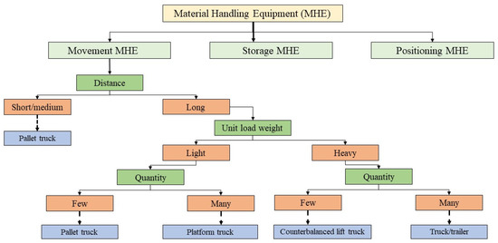
Figure 1.
Selection of MHEs according to the load features.
Transportation, as a logistics function, has progressed positively through standardisation, unitisation, and reduced intermodal handling [9]. Technological advancements in transportation have led to a decline in the compound average growth of transportation costs from a macro-environmental perspective. Despite this, transportation still constitutes the largest share of logistics costs [10].
Transportation networks are integral to enterprise strategy formulation [11]. Table 1 delineates various stakeholders and linkage types in the material flow of a given network, categorised by collaboration levels [12]. Global networks feature nodes connected through transboundary transportation modes like ships, aircraft, and pipelines, characterised by long-term contractual agreements and reduced susceptibility to abrupt changes. In contrast, local networks predominantly employ road transportation modes for delivering materials and goods to customers. Internal networks have shorter planning horizons than global and regional networks, with MHSs facilitating material flows between facilities and departments within the same organisations.

Table 1.
Relationship between supply chain stakeholders related to the material flow.
In addition to basic network configurations, supply chain networks exhibit a range of topological arrangements, each designed to cater to specific operational needs. These configurations include the hub-spoke design, where a central hub serves as a focal point for distribution; the pendulum design, characterised by accommodating reverse supply chain activities; triangle line designs, forming triangular connectivity patterns; and double-dipping service designs, incorporating multiple connecting stakeholders or points [13]. These diverse topologies offer strategic options for optimising supply chain operations based on efficiency, geographic dispersion, and service requirements.
The design of a MHS necessitates inputs and decisions from all levels of management to ensure alignment with the organisation’s objectives. These decisions are grounded in the organisation’s best interests and strategic goals. Figure 2, as presented by Fragapane et al. [14], delineates managerial-level decisions pertinent to MHS design. Additionally, the figure underscores the pivotal role of optimal fleet size as a decision factor influencing all managerial echelons. Notably, the magnitude of the fleet significantly affects criteria for ownership decisions and scheduling considerations at both strategic and operational levels.
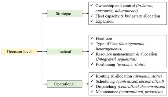
Figure 2.
Decisions areas by each managerial level in the design of an MHS.
Optimisation of MHS operations within an internal network is classified under network optimisation. Ferriol-Galmes et al. [15] delineated the critical components of a network optimisation process: constructing the network model and developing an optimisation algorithm. A plethora of literature exists, presenting techniques for modelling specific networks for analytical purposes. Analytical models, fluid models, and simulators represent well-established tools that emulate intricate systems, such as telecommunication networks, computer networks, manufacturing systems, and healthcare systems. Nevertheless, fluid models exhibit limitations in incorporating queueing delays and scheduling policies, stemming from the assumption that constant per-link delays may compromise accuracy in high-utilisation environments. Additionally, while simulators are acknowledged for their superior accuracy relative to analytical and fluid models, they entail elevated computational costs and extended development times [15]. Queueing networks are a pervasive and widely applied modelling framework in analysing and optimising MHS across diverse operational contexts. This modelling approach is instrumental in comprehensively assessing and refining MHS performance by considering a spectrum of operational considerations [16,17,18,19,20,21,22].
Transportation managers commonly exhibit a predilection for fleet uniformity and commonality due to the enhanced manageability and standardisation these attributes confer upon operations. This preference extends to various operational facets, including maintenance, scheduling, spare parts management, performance monitoring, and cost calculations. The inherent simplicity associated with a homogeneous fleet streamlines these operational aspects, rendering them comparatively more straightforward than their counterparts in a heterogeneous fleet. However, it is imperative to highlight that a heterogeneous fleet introduces distinct advantages, notably heightened operational flexibility. This flexibility translates into tangible benefits, including cost savings and optimised asset utilisation [23]. From an operational perspective, this juxtaposition underlines the nuanced trade-offs that transportation managers must navigate in determining fleet composition, balancing the efficiencies derived from uniformity against the strategic advantages a diverse fleet offers.
This study introduces a novel methodology utilising queueing networks to optimise heterogeneous trucks’ fleet size and composition in internal logistics networks. Building upon the homogeneous fleet optimisation framework established by Amjath et al. [24] in inter-facility logistics, this study extends into the domain of heterogeneous fleet optimisation. A key departure from Amjath et al.’s [24] work lies in the modelling approach adopted here, wherein we employ a CQN featuring heterogeneous nodes. Unlike the previous study’s focus on minimising the total number of trucks, our emphasis centres on optimising operational costs. This shift necessitated the redevelopment of the Mean Value Analysis (MVA) algorithm using S-B approximation to evaluate the performance measures of CQN with heterogeneous nodes, detailed in Section 3.2.
The paper is structured as follows. Section 2 provides a literature review related to the problem addressed in this paper. Section 3 encompasses the problem description, notations, problem formulation, and model development. It also delves into algorithm development, the optimization model, and analytical and simulation approaches. Section 4 offers a case study featuring comprehensive numerical experiments, wherein outputs from the analytical model are validated using the simulation model. Additionally, the section includes sensitivity analyses of selected scenarios and highlights main managerial insights. Finally, Section 5 outlines this research’s implications and concludes with remarks.
2. Literature Review
This section furnishes a comprehensive literature review encompassing three primary domains pertinent to the study problem: (i) fleet sizing problems involving heterogeneous vehicles, (ii) fleet sizing problems employing queueing network models, and (iii) queueing network models specific to MHS. The section concludes by explaining the scientific contributions proffered by this study and identifies anticipated research gaps intended to be addressed.
2.1. Fleet Sizing Problems with Heterogeneous Vehicles
Fleet sizing problems have been widely explored in various transportation and network planning domains [25]. Motivations of fleet sizing studies range from achieving economic and financial objectives such as lower costs and maximised throughput levels to achieving sustainable goals such as reducing emissions and carbon footprints. Moreover, fleet sizing problems are receiving increased logistics attention due to their contribution to costs. Transportation contributes the largest share of logistics costs, and fleet size is an inevitable factor in determining overall transportation costs [10].
This section provides a general overview of researchers’ solutions to heterogeneous vehicle fleet sizing problems. New [26] studied the fleet sizing problem of aircraft acquisition and disposal with budgetary constraints to maximise yield. The author used linear programming to formulate the problem. Etezadi and Beasley [27] presented a study to determine the optimal fleet size and composition for a distribution network to satisfy customer demand while minimising cost. The authors presented integer programming to formulate the problem. Klincewicz et al. [28] studied the problem of a single warehouse distribution network to decide on ownership strategy and the fleet size needed for the distribution operation. Desrochers and Verhoog [29] focused on the fleet sizing problem of a network served by a single distribution centre. The problem was formulated to determine the optimal fleet size and routing to serve all the customers in the network using a heuristic-based approach. Couillard and Martel [30] developed a stochastic programming model to mimic the operations of a trucking company with a seasonal demand to determine the optimal fleet size considering total ownership of cost (TOC). Salhi and Rand [31] developed a heuristics approach to determine the optimal fleet size and mix to minimise routing and acquisition costs while improving the utilisation factor. The authors of [32] conducted a study focused on the problem of fleet sizing and composition with a time window constraint. The authors developed an insertion-based heuristics approach to determine the optimal size and mix of the heterogeneous fleet.
A study by Zhao et al. [33] presented a dynamic programming approach to determining the optimal fleet size and composition for a multi-period distribution network with transhipment hubs. List et al. [34] developed a fleet planning model to identify the optimal fleet size and design considering risk elements. The authors used two-phase stochastic programming to formulate the problem and a decomposition approach to solve the model. Renaud and Boctor [35] used a sweep-based heuristics approach to determine the optimal size, mix, and routing problems with a heterogeneous fleet. Another study focused on developing a methodology to find a cargo rail company’s optimal fleet size and composition. The authors used a queueing network to model the problem considering stationary and non-stationary demand scenarios to determine the optimal rental strategy to improve profitability [36].
Jabali et al. [37] studied a fleet sizing problem integrated with a vehicle routing problem in a distribution network. The authors formulated the problem using the MINLP method and determined the solution’s efficient lower and upper boundaries. Redmer et al. [38,39] proposed a single objective formulation to determine the optimal number of vehicles and size of tankers in a dual-echelon fuel distribution network. The authors used a hybrid algorithm with a local search and evolutionary algorithm to solve the problem. Finally, Roy et al. [40] used the Markovian process to model a transporter network with non-stationary demand and uncertain travel time. The authors used multi-server Markovian queues to decompose the network and determine the optimal fleet size.
Meghjani et al. [41] presented a study on vehicle allocation and optimal fleet sizing of a multi-class heterogeneous autonomous on-demand mobility system. The authors used a genetic algorithm to determine the optimal fleet size of the mobility system with a given budget constraint. Cruz et al. [42] conducted a heterogeneous fleet sizing study integrated with berth allocation and a periodic routing problem for platform supply vessels (PSV) in an offshore petroleum logistics network. The authors used a sequential approach to solve the optimisation problem. Vieira et al. [43] conducted a similar study to determine the optimal size of supply vessels in an offshore logistics problem using the exact and heuristics approaches. The authors used branch and cut frameworks in the solution approach combined with adaptive large neighbourhood search heuristics (ALNS). Fan et al. [44] formulated an optimal fleet sizing problem using the MILP model for an on-demand hybrid mobility system that included both automated and non-automated taxis. The authors considered the profit maximisation objective and solved the fleet sizing problem for a real-life taxi company. Finally, Zhao et al. [45] studied an electric vehicle (EV) system’s network design problem with integrated perspectives from fleet operations and charging services. The study presented a bi-level mixed integer optimisation problem to determine the optimal size of an EV’s fleet and its charging stations capacities and used an iterative approach to solve the problem.
2.2. Fleet Sizing Problems Using Queueing Network Models
Transportation network operators commonly use queueing networks to model transportation systems and analyse fleet performances. Determining the optimal fleet size is crucial due to vehicles’ vast sunk costs. In mobility-on-demand services, optimal fleet sizing is also critical in terms of the profitability of operations and service quality. George and Xia [46] modelled rental car service operations using a CQN to determine the optimal fleet size and maximise profit while maintaining a given service level. Hu and Liu [47] presented a study to assess a car-sharing system’s parking capacity and fleet size considering road congestion and booking policies. The authors used a mixed queueing network to model the car-sharing system and exact and approximate MVA algorithms to solve the system.
Bazan et al. [48] presented a study on the fleet size of a rental car service system using CQNs to maximise the yield. The authors consider the cost of empty vehicle movements when developing the MILP optimisation problem. Iglesias et al. [49] presented a case study using BCMP CQNs to model an autonomous on-demand mobility system in Manhattan and determine the optimal fleet size. The network was used to encapsulate the stochastic behaviour of the mobility system. Kim et al. [50] used an open queueing network to model a car-sharing system. The stochasticity of customer arrival rates and vehicle location dynamics were described through Continuous Time Markov Chain (CTMC) processes. A mathematical model that reflected given circumstances was constructed to determine the optimal fleet size. Similarly, Benjaafar et al. [51] used a CQN to model an on-demand vehicle-sharing system to determine the lower and upper bounds of optimal fleet size to maximise revenue considering given vehicle availability and wait times. First, the authors developed a stochastic optimisation fleet sizing problem considering location randomness and sizes of vehicles. The authors then used closed-form approximation to construct and solve the network.
Fanti et al. [52] conducted a fleet sizing study for an Electric Vehicle (EV) sharing system. The authors modelled the EVs and connected charging stations using CQNs. A discrete event simulation model was developed to determine the optimal EV fleet size and maximise the revenue for minor scale problems. An approximation approach was used with the MVA algorithm to solve queueing networks for more significant issues. In 2020, Fanti et al. [53] extended the solution methodology using a two-level strategy to determine the optimal fleet size. In their study, the authors used a simulation methodology in the first phase and Petri Nets in the second phase to analyse the network. Deng et al. [54] modelled an EV-sharing system using a CQN to analyse system performances. The authors determine the fleet size and the number of charging stations needed in the neighbourhood to maximise profit while minimising operating costs. The authors used the MVA algorithm to solve the network and the Greedy algorithm to allocate EVs to charging stations.
Samet et al. [55] considered the blocking phenomenon and developed a CQN to model a bike-sharing system. The authors used the maximum entropy method to solve the model and determine the fleet size and parking capacities needed to maintain a satisfactory service level. Vishkaei et al. [56] used a Jackson network to model a public bike-sharing system. The authors presented a genetic algorithm approach to determine the optimal fleet size and ensure equilibrium between vacant docks for returning bikes and rejected demand. Finally, Liu and Ouyang [57] used a queuing network to model demand-responsive transportation (DRT) systems and analyse public transportation systems such as the metro, buses, and bus rapid transits (BRT). The transit networks were integrated into the queueing model to estimate the system performances and determine the optimal fleet size for each partitioned zone to achieve a satisfactory service level.
2.3. MHS Queueing Network Models
Performance evaluation and optimisation represent integral facets of system analysis. Queueing networks are fundamental for conducting performance analyses and optimising MHS. Many studies have been dedicated to examining the performance measures of existing systems and assessing the effectiveness of conceptualised systems to inform decision-making processes, employing queueing networks as a modelling framework. The principal performance measures in the domain of queueing network models for MHS encompass cycle times, throughputs, queue waiting times (for both jobs and resources), utilisations, and queue lengths. These measures undergo comprehensive evaluations, accounting for diverse factors such as alternate layout designs, network topographies, population constraints, service disciplines, and queue buffer capacities. Figure 3 illustrates the scope and focus areas of studies of queueing network models within the realm of MHSs.
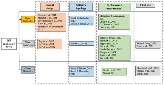
Figure 3.
Study scopes of queueing network models of MHS.
2.3.1. Layout Design Problems
Using MHS queueing network models to analyse and optimise facility layout designs has been widely studied. Heragu et al. [58] and Marchet et al. [59] used queueing networks to compare facility performances with alternate configurations. Roy et al. [60,61] modelled warehouse operations using queueing networks to determine the optimal layout design. Seyedhoseini et al. [62] presented a study to determine the optimal layout design for a cross-docking facility to minimise transportation costs. Xu et al. [63] studied the best layout plan for a manufacturing facility based on resource allocation.
2.3.2. Network Topology Problems
Planning material and customer/job flow are critical to the operational efficiency of material handling facilities. Queueing network models have been used to determine optimal network topologies and manage and measure system performances. Refs. [64,65] used queueing networks to find the optimal topology considering the congestion effect in a warehouse facility. Smith and Barnes studied the optimal topography among selected series, merge, and split configurations for a material handling facility.
2.3.3. Performance Measurement Problems
Performance measurement is one of the challenging tasks faced by material handling operations industry practitioners. Material handling systems queueing network models are a well-known, established tool for measuring systems’ performances, such as throughputs, cycle times, utilisations, queue lengths, and waiting times. For example, Govind et al. [66] determined the work-in-process (WIP) and delay times of MHS in manufacturing facilities. Several research groups have used queueing network models to estimate and optimise systems’ throughput levels for capacity decision-making problems based on various factors in manufacturing and warehouse environments [67,68,69,70,71,72,73]. Similarly, order cycle time is a crucial performance index in material handling environments. Several research groups have modelled order fulfilment operations in warehouse and manufacturing environments using queueing network models while considering operational factors such as service disciplines, resource allocation policies, and layout plans to estimate cycle time [17,74,75,76].
2.3.4. Fleet Sizing (Network Population) Problems
Fleet size, also known as population, is a crucial factor for any given network and plays a vital role in measuring performances when modelling MHS using mixed and CQNs. The number of customers and machines/equipment represents the size of the network population, and the population is a designed consideration in closed and mixed queueing networks. Consequently, the population can be used to achieve desired or maximised throughputs or profitability goals. Choobineh et al. [77] modelled a manufacturing environment using a CQN to determine the optimal number of AGVs and achieve a given throughput. Pascual et al. [78] presented a mining operations case study on asset management related to mobile material handling equipment fleet sizing. The authors used a CQN to model the fork-join cyclical material transportation system. The queueing network model was used to estimate the system throughput, utilisation, and expected wait times. Yuan and Gong [79] and Otten et al. [18] used mixed networks to model RMFS and find the optimal number of robots needed to achieve service levels in a warehouse. Munoz and Lee [80] conducted a study to determine the optimal number of trucks for a sugarcane harvesting field by modelling operations using a CQN.
2.4. Scientific Contribution and Research Gaps in Fleet Sizing
This section outlines the scientific contributions of the study and articulates the specific research gaps it seeks to address. The existing literature has demonstrated the utilisation of queueing networks in modelling fleet sizing problems within the realm of on-demand mobility systems, notably in contexts like car-sharing, EV-sharing, and bike-sharing systems. This study’s contribution extends the application of queueing network models to a new domain, addressing the challenges inherent in optimising a heterogeneous truck fleet within an interfacility MHS context.
The existing literature on queueing network models for MHS fleet sizing problems is limited. Choobineh et al. [77] optimised AGV fleet size in warehousing, considering service levels and throughput, while Pascual et al. [78] maximised yield in mobile material handling equipment for mining. Both studies applied a decomposition approach, assessing performance metrics like waiting time, utilisation, throughput, and queue lengths. Fleet size, treated as a continuous variable, was optimised using a linear programming framework by Choobineh et al. [77], with a subsequent rounding step for practical implementation.
Yuan and Gong [79] focused on determining optimal fleet sizes for mobile robots and AGVs in warehouse operations to maximise throughputs. In a separate context, Munoz and Lee [80] studied the optimal number of trucks for sugar cane harvesting to minimise idle time. Both Yuan and Gong [79] and Munoz and Lee [80] employed single-class mixed and CQNs to model material handling operations. Notably, all these studies are confined to optimising homogeneous fleets within MHSs.
Amjath et al. [81] investigated the optimisation of MHS using CQN and employed simulation as an optimisation tool. The study introduced a mathematical model solved through the Anylogic optimisation engine utilising meta-heuristics. Notably, this study needs to have an analytical method for optimisation, relying solely on simulation optimisation, potentially raising concerns about computational efficiency and accuracy with larger-scale problems. In a parallel vein, [82] addressed supply chain challenges through three research projects, employing agent-based modelling (ABM) and network optimisation. The first project focuses on optimising Distribution Center (DC) locations in the Nordic region, while the second introduces ABM for transportation cost modelling in tree log collection. The third project utilises ABM for vehicle scheduling and fleet optimisation, leveraging real-world organisational data. The recognised customizability of the ABM methodology is showcased as instrumental in a comprehensive assessment and enhancement of supply chain efficiency. Bebortta et al. [83] presented an optimal fog-cloud offloading framework for Internet of Things (IoT) networks with heterogeneous loads in a broader context beyond logistics. The authors introduced a dynamic Integer Linear Programming (ILP) technique to optimise task offloading, efficiently distributing resources from the fog computing layer to IoT devices while constraining on-time execution and availability of resources.
This study represents an extension of the work conducted by Amjath et al. [24], which primarily addresses fleet size optimisation for homogeneous trucks in inter-facility operations. In contrast, the current investigation assumes a specialised perspective, dealing with a fleet characterised by distinct carrying capacities, service times, and operational cost characteristics. The algorithms employed in the previous study needed to be revised to address the intricacies inherent in this specialised scenario. The scientific contribution of this study lies in its departure from the generic, offering a framework and algorithms with broader applicability. These advancements can address networks with heterogeneous nodes, thereby accommodating diverse operational and design attributes. Consequently, this work establishes a foundation for comprehensive solutions within broader, heterogeneous operational contexts.
Table 2 summarises works similar to this study and shows the research gaps expected to be filled by this study.
Table 2.
Similar studies scopes, methodology and solution approaches.
3. Methodology
This section delineates the methodology employed in formulating a modelling and solution approach for a fleet sizing problem within an inter-facility MHS governed by a heterogeneous fleet of trucks. Furthermore, the subsequent subsections explicate the methodology adopted in a phased manner. These phases encompass modelling, analytical techniques, optimisation approaches, validation methodologies, and analytical modules.
3.1. Modelling Approach
The optimisation of MHS operations within an internal network fall within the domain of network optimisation. Ferriol-Galmes et al. [15] delineate the principal components of the network optimisation process, encompassing the construction of the network model and the development of an optimisation algorithm. In alignment with these principles, this study has chosen CQN to model inter-facility material transfer operations for subsequent analysis and optimisation. Figure 4 illustrates the strategic roadmap for selecting this study’s modelling tool and solution approach.
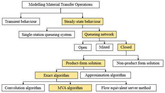
Figure 4.
Roadmap for selecting a modelling and solution approach for the problem.
This investigation is centred on elucidating the steady-state behaviour of the network, particularly in the context of interfacility material transfer processes characterised by multiple sub-processes. Given that a singular station queueing system fails to adequately meet the modelling requirements due to the presence of distinct nodes representing these sub-processes, a queueing network becomes the chosen modelling approach. The specificity of interfacility material transfer, where the vehicles involved do not exit the system, necessitates the application of a CQN. In order to streamline the modelling process, the study assumes a product-form solution for the network, and the MVA algorithm, selected for its efficiency, is employed to solve the system. The MVA algorithm’s recurrent use in CQN performance measurements is attributed to its computational efficiency and the circumvention of normalising constant calculations denoted by G (N, k).
3.2. A CQN for an Inter-Facility Material Transfer Operation with a Heterogeneous Fleet of Trucks
The daily occurrence of inter-facility material transfer operations, involving the transportation of multiple materials between storages and intermediate production facilities, necessitates the engagement of an outsourced heterogeneous fleet of trucks. The heterogeneity in truck characteristics, including capacity (throughput), service times (e.g., loading, unloading), and operational costs, coupled with the diverse physical attributes of each material, leads to variations in total truckload weights and service times. Distinct materials also prompt trucks to follow different routes and receive service at specific stations. The material flow sequence of a truck begins at a service station, progresses through subsequent stations sequentially, and encounters specific tasks and responsibilities at each. Two primary classes categorise service stations: those dedicated to a single product class and those accommodating multiple product classes.
In the context of a service station exclusively serving a single product class, it functions as a single-class heterogeneous node within the network. Here, service and waiting times for trucks depend on the truck type. Upon a truck’s arrival at such a node, two scenarios unfold: direct service if the station is unoccupied, with service duration contingent on the truck type, or queueing if the station is occupied, with waiting time determined by the type of truck currently undergoing service. The mathematical representation of this phenomenon is encapsulated in the first equation of our analysis. It is imperative to note that, in this framework, we assume infinite queue capacity across all service stations, eliminating instances of blocking. Equation (1) effectively elucidates the derivative of the total response time for a truck within a single-class heterogeneous node.
If a service station accommodates more than one product class, it assumes the role of a multi-class heterogeneous node within the network. In this scenario, when a truck (customer) arrives at the station, the response time is contingent upon both the product class and the type of the truck. Here, it is plausible for a truck to be serviced from the same product class but with a different truck type or, conversely, from a different product class with a distinct truck type. Consequently, in multi-class heterogeneous nodes, the incoming truck’s product class and truck type jointly influence the response time of the node in relation to the trucks. Equation (2) comprehensively delineates the constituent components of the response time for a truck within a multi-class heterogeneous node.
Single-class heterogeneous node’s response time:
Multi-class heterogeneous node’s response time:
According to Figure 5, the response time for the truck (k, t) in service station j is the summation of the service time of the truck (k, t) and the wait time, as in Equation (1) for single-class heterogeneous nodes. The wait time can be elaborated upon further as in Equation (2). If a service station is used by multi-class trucks, the wait time can be attributed to different classes and types of trucks.

Figure 5.
Node configuration for response time calculation.
In this logistical context, several foundational assumptions underpin the operational dynamics of the system. Firstly, service times at all service stations are assumed to follow an exponentially distributed probability distribution, enabling the modelling of service duration variability. Queue management adheres to a first-come-first-served (FCFS) discipline. A stringent class persistence policy is enforced, prohibiting trucks from switching between product classes within the same time frame. The intermediate production facility reliably meets material requirements on a regular operational day. A structured operational sequence is defined for each truck: arrival and documentation at the storage yard gate, weighbridge recording weights of empty trucks, loading at the station, recoding weights of loaded trucks and subsequent transportation to the facility for unloading. This cycle continues until the intermediate facility’s demand is met. During transit from loading to unloading, trucks are fully loaded, and on the return journey, they are empty.
Based on the model formulation and assumptions above, each service station is modelled as M/M/1 with an infinite queue capacity, and circulation between service stations is modelled as M/M/∞. As mentioned earlier, this study uses the parametric decomposition approach to solve the CQN using the MVA algorithm. The following nomenclature was introduced for algorithm development and mathematical model formulation.
The following part provides the steps for tailoring the MVA algorithm to this study using the work of Suri et al. [84] and Smith and Kerbache.
According to Reiser and Lavenberg’s [85] proof of the arrival theorem, the response time of a customer arriving at a node is equivalent to the summation of the customer’s service and wait times amalgamated from all of the customers already in the network minus one. Therefore, the following is the response time of a truck (k, t) in the service station j, where j is only used by class k and served by a single server:
Equation (3) can be extended to calculate the mean response time of a truck (k, t) in the service station j, where service station j is used by all classes and served by a single server, using the Schweitzer–Bard (S-B) approximation [84].
According to Little’s Law for product chains, the network throughput of class k type t trucks is:
Moreover, from Little’s Law for queues, the mean queue length of class k type t trucks at station j is:
According to Suri et al. [84], the utilisation rate of truck type t for product class k in a single server service station j is:
The cycle time for a truck is the summation of all the service times in one trip. However, a truck visits only certain service stations along the trip according to the product class it carries. Therefore, a binary variable is included to ensure that service times from the service stations visited are only used to calculate the cycle time for a particular type of truck for a product class. The cycle time for truck type t for product class k can be written as follows.
Equation (8) can be re-written as follows by substituting the from Equation (4):
For all classes,
3.3. Formulation of the Optimisation Problem
Fleet sizing is integral to the decision-making processes regarding outsourcing MHEs to an organisation. Moreover, determining the right size and composition from heterogeneous equipment fleets is more challenging because of each piece of equipment’s cost, capacity, and other operational factors varies. Similarly, determining the optimal number of trucks and composition from an available heterogeneous fleet is a complex decision-making problem.
This study focuses on minimising the outsourcing cost of the interfacility transportation process. The outsourcing cost depends on the number and types of trucks the organisation plans to acquire and is pro rata for the same truck. Therefore, the total price is an aggregate product of the number of a particular variety of trucks outsourced into the cost of that truck. Generally, the logistic and transport managers’ objective is to outsource the right kind and number of trucks to ensure the smooth flow of materials to the buffer locations. Moreover, the optimal fleet size and composition are bounded by the total available budget and a time window.
The decision variable and surrogate variable are as follows:
Number of type t trucks used for product class k
Cycle time for truck type t product class k with N number of trucks
The objective function is as follows:
and is subject to the following constraints:
Equation (11) can be re-written using the surrogate variable as follows.
The objective function (Equation (11)) is linear and minimises the outsourced trucks’ total cost (Z). The first constraint (Equation (12)) is an allocation constraint where one truck must be allocated to either only a single type of product class or unassigned. The second constraint (Equation (13)) is non-linear and ensures that demand from the intermediate buffer locations is met for each product class within the provided time window. This constraint is notable because the decision variable is present in the numerator and influences the values in the denominator through the surrogate variable (Equation (17)). Equation (14) is a linear knapsack constraint that bounds the number of trucks to an available budget. The fourth constraint (Equation (15)) is a capacity constraint for each product class at the intermediate production facility that needs to be respected. Equation (16) shows that the decision variable is a positive integer and is a real positive variable.
3.4. Solution Approach for Solving the Mixed Integer Non-Linear Optimisation Problem
Determining the optimal network population in a CQN for a given throughput under the queue discipline of non-pre-emptive policies is an NP-Hard problem [86]. This study problem, determining the optimal fleet size and composition using a CQN model, falls within the NP-Hard category. Therefore, obtaining solutions using exact algorithms in a polynomial time is unfeasible. Consequently, finding efficient solutions for these problems requires numerical approximation approaches and heuristics. Implementing a modified Sequential Quadratic Programming (SQP) method is one of the most powerful and efficient tools to solve mixed integer non-linear optimisation problems. Schittkowski [87] presented an SQP method for solving a non-linear constrained optimisation problem with a Fortran subroutine NLPQL. This method assumes integer variables have a smooth influence on model functions, resulting in only marginal decrement or increment in the function value with the change of an integer value. The solution to the quadratic programming subproblem is to convert the objective function and constraints to a quadratic problem and then use iteration to determine the search direction. The main steps of implementing an SQP method for this study are as follows.
- Step 1.
- Set the initial parameter and constant values.
- Step 2.
- Implement a branch and bound method with several branching and node transversal strategies. Then, as an unconstrained problem, evaluate the objective function (using the MVA algorithm) to determine the minimizer for the relaxed problem.
- Step 3.
- Using the solutions from the previous step, evaluate the objective function values while adding violated constraints.
- Step 4.
- Evaluate the objective functions using the primal-dual method by incorporating Lagrangian multipliers and partial derivatives to find the direction of the optimal solution vector for the relaxed problem.
- Step 5.
- Using the convergence solution from the previous step, create two sub-problems with integer values using lower and upper bounds from the continuous solution.
- Step 6.
- Evaluate the objective function value using the new sub-problems and check for convergence. If there is no convergence, repeat Step 4 to find a new solution. Otherwise, terminate the process.
The above steps are shown in the following flowcharts to show the roadmap of the solution approach in a visual form. The final solution from each flowchart is the starting point for the following chart. Figure 6 shows the steps to create a binary search tree for the relaxed constraint problem. The binary search tree is used in the next phase of the solution approach to determine optimal solutions while adding violated constraints step-by-step and evaluating the new solution. In this phase, the problem is solved as a non-integer (continuous) optimisation problem.
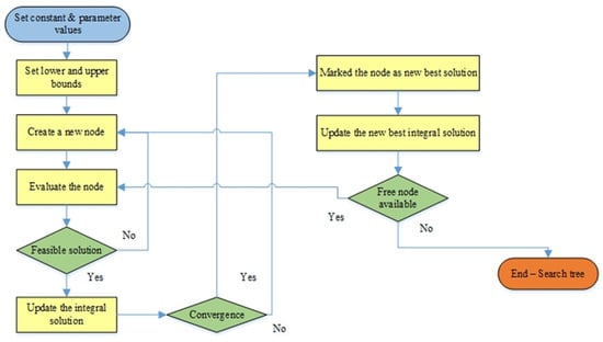
Figure 6.
Flowchart for finding the binary search tree with relaxed constraints.
Figure 7 shows the steps of solving the problem to obtain continuous solutions. Finally, through the lower and upper integer bounds of the continuous solutions, sub-problems are created and evaluated to find the optimal solution. Figure 8 shows the steps for finding the integer solution for the non-linear constrained optimisation problem.

Figure 7.
Flowchart for obtaining optimal continuous solutions.
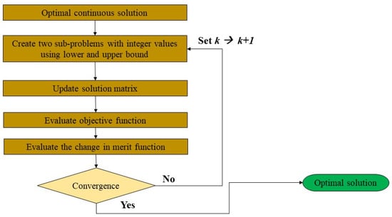
Figure 8.
Flowchart for evaluating functions to find the optimal integer solution.
In this study, the Fortran MISQP subroutine was used to implement the SQP method and solve the optimisation problem. As a subroutine, the main program, called the MVA algorithm, is used to solve the queueing network and find the performance measures. All the experiments were conducted on a PC with Intel(R) Core i3-7100U CPU 2.40 GHz, 4.00 GB RAM.
3.5. Discrete Event Simulation Model
In this study, Anylogic Simulation Software 8.7.7 University edition was used to construct a DES model, ensuring methodological rigour regarding stability and model validity. Figure 9 shows the process map of developing a DES model for study. Utilising blocks from the process modelling library, the simulation model incorporated fundamental components detailed in Figure 10. Figure 11 elucidates the configuration options for agents, offering a foundational description.
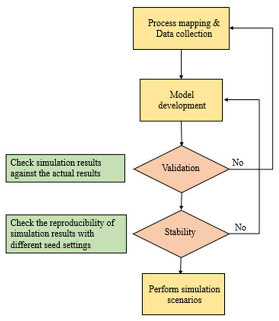
Figure 9.
Process flow for DES model development.
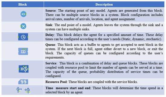
Figure 10.
Basic simulation blocks and descriptions.
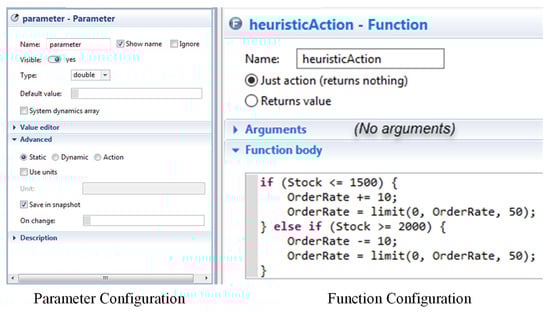
Figure 11.
Configuration components of an agents in Anylogic software 8.7.7 University edition.
The parameter component was pivotal in assigning values to agents based on specified requirements, encompassing cost, speed, and capacity. This component facilitated versatile parameterisation by Accommodating Boolean, integer, double, rate, string, and user-defined types. The variable component interfaced with agents, defining dynamic variables like stock levels influenced by agent activities. The function component introduced functionality to incorporate optimisation models, enabling users to establish requirements linked to optimisation experiments for maximisation or minimisation objectives.
AnyLogic’s simulation software implemented successive iterations and metaheuristic approaches for optimisation experiments. The OptQuest Optimisation Engine, integral to AnyLogic’s optimisation tool, harnessed metaheuristics to guide the search algorithm toward optimal solutions. The formulation of optimisation problems involved specifying the objective function, decision variables, constraints, and constraint relaxations through designated tabs, as exemplified in Figure 12. Users determined iterations and allocated memory, tailoring the experiment to accuracy and computation time requirements.

Figure 12.
Optimisation experiment window in Anylogic software.
The optimisation experiment within the ambit of AnyLogic simulation was executed by deploying the OptQuest optimisation engine. This advanced engine harnessed the power of successive iterations and metaheuristic methodologies, strategically navigating the solution space to glean optimal outcomes. The temporal dynamics of the simulation model were orchestrated with precision, spanning a temporal expanse of 20,000 units. A warm-up period of 1000 units was incorporated within this timeframe to ensure the model’s equilibrium before initiating data collection. The reliability and robustness of the results were ensured through the simulation experiments conducted over 20 replications, thereby encapsulating a comprehensive and statistically sound exploration of the system dynamics. This methodological configuration aligns with best practices in simulation experimentation, ensuring a nuanced and reliable analysis of the simulated logistics scenario.
Upon the entry of an agent (truck) into the system, each service block undertakes the crucial task of discerning the truck’s type and the associated product class it carries. Individual trucks exhibit distinct attributes, including carrying capacity, cost, and loading and unloading times. Concurrently, each product class is characterised by unique attributes such as density, demand, and service times at each station. Subsequently, the simulation process involves calculating costs, demand fulfilment for the identified product class, and time allocation. This iterative process continues throughout the cycle. User input imposition of budget, time, and demand constraints becomes imperative. By specifying constraints, the simulation model generates performance metrics for the identified scenarios, offering insights into the system’s dynamic behaviour and efficiency under various conditions (Figure 13).

Figure 13.
Back-end process of a service block in the simulation model.
4. Steel Manufacturing Case Study—Numerical Experiments
SM manufactures steel rebars of various quality grades according to customer requirements. SM procures its raw materials from domestic and overseas suppliers. There are three major types of raw materials (A, B, and C) SM stores in its storage yards to produce steel billets. In the final processing phase, steel billets are converted into steel bars. Due to storage capacity limitations at the intermediate manufacturing facility, raw materials are stored in a storage yard near the facility (Figure 14). Each material in the storage yard has a 1200-ton capacity dedicated space. Transportation between the storage yard and the intermediate manufacturing facility is operated by outsourced trucks.
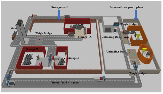
Figure 14.
Layout plan of all node points in an SM facility.
At the start of every day, the production plant informs the storage yard of the material required for that day’s production. Then, according to the day’s requirement, the logistics manager hires the required number and type of trucks to ensure the smooth feed of materials to the plant. In a typical forward flow, a truck goes through many processes, such as documentation, weighing, loading, security clearance, quality check, and unloading. The process map, service station’s node markings, and service times are presented in the Appendix A (Figure A1 and Table A1 and Table A2).
The heterogeneous fleet engaged in interfacility material transfer operations exhibits variations in cost, carrying capacity, and loading/unloading service times. A delineation of the distinct characteristics of this heterogeneous fleet is provided in Table 3.
Table 3.
Heterogeneous fleet of trucks’ specifics.
Figure 15 was designed to illustrate the problem as a CQN representation. Within this visualisation, the service times are juxtaposed with the salient features of the network nodes. This graphical representation offers a comprehensive and holistic perspective on the case study problem’s intricacies. It aids in elucidating the interplay between service times and the specific characteristics of the network’s constituent nodes, facilitating a deeper and more intuitive understanding of the problem within the broader context of queuing theory and network optimisation.

Figure 15.
SM interfacility material transfer operations as a multi-class CQN.
The production plant bill of materials (BOM) requirements depend on factors such as committed customer orders, available raw materials in the market, and prices. The management decides the production plan using their information about the above factors. The management then provides the BOM for that day to the storage to feed the intermediate production plant.
Table 4 shows different BOM requirements from the plant to the storage yard for a 12 h shift. This study’s numerical experiments were carried out for the following identified BOM scenarios.
Table 4.
Different BOM scenarios for experiments.
4.1. Numerical Experiments Results Analysis and Validation
This section presents the outcomes of numerical experiments conducted on the scenarios outlined in Table 4, utilising the analytical model. The results are validated through a comparison with outputs from the simulation model. Initial calculations involved determining the optimal number of trucks and compositions using the analytical method, subsequently verified against the simulation model. Performance metrics, including response times, utilisations, and queue lengths, were estimated through the analytical approach, and meticulously compared with simulation model outputs to gauge the method’s robustness. Subsequently, the algorithm’s performance was scrutinised under varying conditions to assess its resilience. A succinct set of sensitivity analyses were also performed, furnishing insights pertinent to decision-making processes.
4.1.1. Optimal Number of Trucks and Compositions
Table 5 and Table 6 present the optimal truck quantities and compositions derived from the analytical method and simulation model for each scenario outlined in Table 4. A DES model (Figure 16) emulating the SM case study employed the simulation’s built-in optimisation black box. Table 5 details the optimal truck allocation, composition, and the number of functions evaluated using the analytical method, utilising an SQP method that employs branch and bound techniques for integer point evaluations. Table 6 mirrors the optimal truck allocation and composition obtained from the simulation model and the corresponding number of iterations. This comparison serves to validate the accuracy of the analytical method’s solutions.
Table 5.
Optimal truck allocation and composition by analytical method.
Table 6.
Optimal truck allocation and composition using the simulation model.
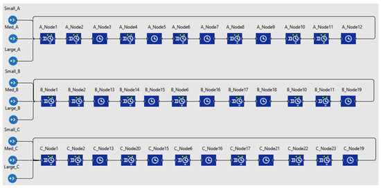
Figure 16.
Simulation model for the SM interfacility material transportation process.
Table 7 presents a comparative analysis of objective function values and computation times between the analytical and simulation methods, validating the analytical approach’s accuracy and efficiency. The objective function values, expressed in dollars, are meticulously documented for each scenario, showcasing the optimal solutions derived from both methodologies. Additionally, the computation times, measured in seconds, provide a critical insight into the time efficiency of each strategy.
Table 7.
Comparison of objective function values and computation times for analytical and simulation methods.
Upon examination, it is evident that the analytical method consistently yields objective function values corresponding to the optimal solutions, affirming its robustness in addressing the fleet sizing optimisation problem. Moreover, the analytical method demonstrates superior computational efficiency when juxtaposed with the simulation method. Notably, the computation time for the analytical method remains notably lower across all scenarios, underscoring its proficiency in delivering swift and precise results.
Optimisation experiment settings were configured for a maximum of 5000 iterations in the simulation method, thereby standardising the computation time for all scenarios within the simulation experiments. This standardised setting facilitates a fair and comparable assessment of the two methodologies, emphasising the analytical method’s reliability and efficiency in solving complex fleet sizing optimisation challenges.
4.1.2. Comparison of Response Times
The analytical approach, leveraging the MVA algorithm detailed in Section 3, employs Equations (3) and (4) to calculate mean response times for single and multiple class nodes. In parallel, the simulation model implemented in the AnyLogic software features an integrated code mechanism designed explicitly for computing mean response times within a given service block.
Table 8 systematically contrasts the response times obtained through the analytical and simulation methodologies, focusing on selected single-class use nodes. The disparity between the two methods is quantified using Equation (18), facilitating a precise evaluation of their alignment. The resultant difference column illustrates that the outputs generated by the analytical method consistently fall within an acceptable margin compared to simulation outputs, as depicted in Figure 17. Notably, the calculated differences are limited to ±8%, underscoring the analytical method’s capacity to furnish outputs of commendable accuracy in determining queue response times.
Table 8.
Response time comparisons on selected single-class nodes.
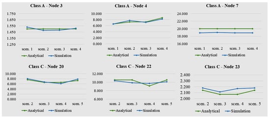
Figure 17.
Queue response time comparisons for single-class nodes.
Table 9 presents a comprehensive comparative analysis of queue response times between the analytical and simulation methods, explicitly focusing on selected multi-class nodes. The differences between these methodologies have been quantified by applying Equation (18). Furthermore, the calculated difference range serves as a critical metric to assess the acceptability of the disparities, adhering to the predefined criterion of ±8%. This rigorous evaluation aims to affirm the efficacy of the proposed analytical methodology.
Table 9.
Comparison of queue response times for multi-class nodes.
The outcomes, as depicted in the tables (Table 8 and Table 9), conclusively demonstrate that the mean queue response times obtained through the suggested analytical method, both for single-class and multi-class nodes, exhibit a commendable level of accuracy. This proximity of results substantiates the effectiveness and reliability of the analytical approach in accurately estimating queue response times across diverse operational scenarios.
Moreover, in the context of single-class nodes, response time deviations are marginally lower than those of multi-class nodes (Figure 18). Furthermore, the analytical method exhibited slightly superior performance in calculating queue response times for circulation nodes (nodes 13 and 19) than for resource nodes (nodes 2, 6, 11, and 10). The difference ranges for circulation nodes were less than ±3%.
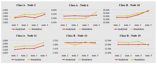
Figure 18.
Queue response time comparison for multi-class nodes.
4.1.3. Comparison of Utilisation Rates
Utilisation rates serve as crucial performance indicators in operational systems, and their assessment and management are paramount for continuous process improvement. Within the MHSs context, resource utilisation rates are vital in evaluating, controlling, and enhancing system efficiency. In the inter-facility material transfer process studied here, various resources were strategically allocated to cater to the service needs of trucks. Resources such as gates, weighbridges, and security offer uniform services to all trucks, regardless of type or product class, resulting in similar service times. Conversely, resource pools like loading equipment, quality inspection, and unloading equipment may deliver distinct services based on truck types and product classes.
The analytical method, employing Equation (8), was utilised to calculate utilisation rates, while the simulation model employed an in-built command line for the same purpose. Table 10 provides a comparative analysis between the analytical method and simulation model outputs for selected resource nodes in identified scenarios, with differences quantified using Equation (19).
Table 10.
Comparison of utilisation rates for analytical and simulation methods.
Table 10 delineates the disparity analysis between outputs derived from the analytical and simulation methods, revealing a consistent range of −2% to −8%, barring a solitary exception. Elevated differences tend to manifest in service station nodes exhibiting high utilisation levels. For instance, in scenario 4, node 10, registering a 0.989 utilisation rate through the simulation method elicited a discrepancy of approximately −12% in the analytical method. This phenomenon aligns with the established literature, indicating that the MVA algorithm may exhibit relative weakness in networks with node utilisation rates approaching 1.0 within CQN non-priority queue disciplines [86]. Such close proximities to 1.0 signify congested nodes, acting as potential bottlenecks within the system. Timely identification of these bottlenecks aids managers in proactively reshaping systems to avert operational standstill. The proposed analytical methodology consistently furnishes highly accurate utilisation rate estimations, robustly validated against simulation outputs.
4.1.4. Comparison of Cycle Times
Cycle time, a pivotal metric guiding the optimal deployment of trucks for distinct product classes is subject to rigorous comparison between analytical and simulation methodologies in Table 11. This tabulated data underscores the close alignment between outputs from the analytical method and simulation, with discrepancies confined within the narrow band of approximately ±7%. The findings robustly affirm the analytical method’s competence in delivering accurate mean cycle times, substantiating its reliability in operational scenarios. The disparity between analytical and simulation outputs is quantified by Equation (20), elucidating the negligible divergence within the stipulated range.
Table 11.
Comparison of mean cycle times for all scenarios.
4.1.5. Performance of the Optimisation Algorithm
This section delineates the performance evaluation of the numerical SQP approach for solving mixed-integer non-linear optimisation problems. Table 5 provides a comprehensive overview of the optimum results of the proposed analytical method substantiated through simulation optimisation experiments. The analytical methodology, proven to be a robust tool, demonstrates efficacy in swiftly resolving large-scale problems.
As delineated in Table 5, the quantity of functions evaluated during the optimisation process emerges as a pivotal determinant influencing the algorithm’s performance. This section scrutinises the performance of the proposed methodology by considering two crucial factors: the lower and upper bounds of the solution and the initial solution. The ensuing analysis, elucidated in Table 12, encapsulates the optimal solutions achieved under diverse conditions for these specified factors.
Table 12.
Optimal solution comparison with varied lower and upper bound values.
Establishing a judicious range for lower and upper bounds in optimising the solution enhances the algorithm’s efficacy. The absence of an upper bound typically leads to a sluggish algorithmic performance, precipitated by the need for an exhaustive search and the subsequent generation of an expansive search tree. Consequently, this amplifies both computation time and the number of functions evaluated. Moreover, introducing an upper bound contributes to the convexity of the objective function.
In the context of scenarios 1 and 2, the presented algorithm underwent rigorous testing against augmented upper bounds to assess its resilience. Encouragingly, the algorithm demonstrated robust functionality with the expanded upper bounds, affirming that the increased bounds did not compromise the number of functions evaluated or the computation time.
Figure 19 visually depicts the influence of initial solutions on the algorithm’s performance, providing insights into the algorithm’s responsiveness to different starting conditions. The illustration encompasses the representation of the original search’s initial solution, along with the incorporation of two novel starting solutions aimed at assessing algorithmic performance under varying circumstances. One initial solution has been strategically positioned in proximity to the optimal solution, while the other has been deliberately situated at a considerable distance from the optimum. This deliberate selection of divergent starting points allows for a comprehensive examination of the algorithm’s robustness and adaptability across a spectrum of initial conditions, shedding light on its efficacy under favourable and challenging scenarios. Exploring these distinct starting solutions contributes valuable insights into the algorithm’s sensitivity to the initialization phase and ability to converge toward optimal outcomes.
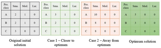
Figure 19.
Initial solution scenarios for optimisation algorithm performance analysis.
Table 13 presents a comprehensive output analysis for both cases, interpreting the algorithm’s performance under distinct initial solution scenarios. The findings reveal a notable correlation between the proximity of the initial solution to the optimum and the algorithm’s efficiency. Specifically, the algorithm demonstrates expedited performance when initiated closer to the optimum, manifesting in a discernible reduction in computation time and the number of evaluated functions.
Table 13.
Effect of initial solution on the computation speed of the algorithm.
Notably, the results in Table 13 showcase that, in Case 2, where the initial solution is distanced from the optimum, the number of evaluated functions escalates from the initial 121 to 240, and the computation time experiences a substantial increase of 6.5 s. In contrast, Case 1, characterised by a closer initial solution, demonstrates a reduced evaluated function to 96 and improved computation time by 0.8 s. Despite these variations, it is noteworthy that the optimisation algorithm yields identical optimum objective function values for both cases.
This underscores the algorithm’s ability to converge to the optimum even under diverse starting conditions while emphasising the critical impact of the initial solution’s proximity on computational efficiency and resource utilisation. Notably, the non-convergence issue becomes evident when the initial solution is significantly distant from the optimum, underscoring the algorithm’s sensitivity to the initialisation phase.
4.2. Sensitivity Analysis
Sensitivity analysis is an indispensable instrument in decision-making processes across various managerial echelons, offering a nuanced examination of the repercussions associated with contemplated alterations in processes or resource allocations within a given setup. In this context, the present section delves into the ramifications of assigning multiple servers to congested nodes as a strategic intervention to enhance operational efficiency. The investigation meticulously observes changes in improvements in response times within service stations, optimal objective function values, and utilisation rates. Furthermore, an in-depth analysis is conducted on Bill of Materials (BOM) scenarios to minimise material transportation costs. In each scenario, graphical representations delineate material requirements concerning total material demand and transportation costs, facilitating the identification of optimal configurations. This holistic approach provides valuable insights for decision makers by systematically assessing the multifaceted impacts of varying operational parameters on critical performance metrics within the system.
In Scenario 4, the utilisation rates for Node 10 were meticulously estimated at 98.9%, as outlined in Table 10. This node caters to both class A and B trucks. A node’s utilisation rate nearing 100% indicates a system bottleneck, necessitating strategic intervention. In order to ameliorate congestion, the operational process must undergo a redesign, or the number of servers at the corresponding service station should be augmented. The bottleneck issue at Node 10 demands a proposition that involves introducing an additional server, enabling the concurrent servicing of two trucks. In alignment with the optimal truck allocation, five small trucks for class A and three small trucks for class B were allocated, resulting in a total objective function value of $1070.
Table 14 presents the enhanced performance metrics of the reconfigured setup, illustrating improved response times, utilisation rates, and objective function values. Notably, the optimised truck allocation objective function experienced a significant enhancement, reducing from $1070 to $1000. Simultaneously, response times for class A and class B trucks demonstrated reductions to 9.92 and 10.09 min, respectively. The mean service station utilisation rate exhibited a notable drop to 53.9%. This strategic adjustment effectively addresses the bottleneck issue, optimising system efficiency and resource utilisation, as the refined performance metrics substantiate.
Table 14.
Effect of assigning an additional server in node 10, scenario 4.
Figure 20 presents 3D surface plots that intricately illustrate the interplay between each material class’s requirements, the total transportation cost, and the aggregate material requirement within the system. All scenarios considered within this visualisation maintain a constant total material requirement of 1800 tons, enabling a discerning examination of cost variations corresponding to changes in individual material requirements. Notably, the surface plots unveil nuanced relationships; for instance, as depicted in Figure 17, a reduction in the material requirement for class C correlates with an increase in the total transportation cost. Conversely, an augmentation in the material requirement for class A yields a parallel increase in total cost. Material class B exhibits a more intricate pattern, demonstrating a mixed response to material requirements variations and associated costs.

Figure 20.
Three-dimensional surface plots with different material requirements against total requirements and costs.
Moreover, increments in the aggregate of materials A and B consistently result in corresponding increases in the total cost. Intriguingly, the transportation perspective attains optimal efficiency with higher material C requirements. This multifaceted analysis not only enriches our understanding of the intricate cost dynamics within the system but also provides nuanced insights into the varied impacts of individual material class requirements on the overall transportation costs, thereby contributing to a more refined decision-making framework.
4.3. Managerial Insights
Table 5 presents the optimal allocation and composition of trucks for different material classes, revealing a consistent preference for heterogeneous fleets in all scenarios. The data underscore the economic and asset utilization advantages of employing diverse truck types, mainly when dealing with the intricacies of transporting mixed products. However, the decision-making process is intricate due to the myriad combinatorial options inherent in heterogeneous fleets, compounded by multiple product classes’ shared usage of certain service stations. As shown in Table 5, the material requirement and truck allocation for classes C (scenarios 1 and 2) and B (scenarios 3 and 4) are identical. The material requirements for classes B (scenarios 1 and 2) and A (scenarios 4 and 5) are different, but the optimum truck allocations are the same. Therefore, it is understood that optimum solutions are distinctive according to the requirements.
The material required for class A increased from scenarios 1 to 5, and the total cost increased for all the scenarios except for scenario 5 (see Table 5). Generally, it is observed that when the class A requirement increases, the total cost increases. However, this could be a misleading conclusion since, when scenarios 4 and 5 are compared and the total cost of scenario 4 is higher than scenario 5, the class A requirement is higher for scenario 5. Therefore, managers must understand that they need views of all network situations when engaging in decision-making processes. The sensitivity analysis part, the multi-server case, further strengthens the point of analysing things holistically. Table 14 shows that node 10 response times reduced for classes A and B improved with allocating an extra server. However, the truck allocation and composition remained the same. Surprisingly, the truck allocation changed for class C due to the improvement in node 10. It switched from 1 large truck to 2 small trucks, giving a $70 cost advantage. This further highlights the need for a holistic approach to analysing systems for managerial decision making.
In summary, Logistics managers must adopt a systemic view, avoiding isolated improvements that may inadequately address performance issues. Operations should be studied as an interconnected whole, informing continuous improvement initiatives. Since all these processes were directly or indirectly connected, they should be studied and analysed as a whole system to achieve continuous process improvements. Moreover, planning teams can use this information related to the fleet sizing problem in their mid- and long-term planning of capacity capabilities when drafting master plan schedules and material requirement plans.
5. Conclusions, Implications, and Future Extensions
In conclusion, the ubiquitous preference for homogeneous fleets in logistics operations stems from their inherent advantages in operational simplicity, crew management efficiency, resource allocation optimisation, spare parts management streamlining, maintenance scheduling, and performance measurement. These attributes render uniform fleets an appealing choice for diverse logistics activities. However, the operational intricacies of scenarios involving materials with distinct physical attributes underscore the efficacy of heterogeneous fleets. The strategic utilisation of diverse features within a fleet facilitates more efficient multi-commodity transportation operations, enhancing overall operational efficiency. Whether engaged in manufacturing or services and contemplating the acquisition of transportation resources from third-party logistics (3PL) providers, organisations must meticulously evaluate their fleet size and composition to optimise operations, ensuring operational excellence and profitability.
This study explicitly addresses the intricate challenge of determining the optimal allocation and composition of heterogeneous trucks for interfacility material transfer operations obtained from a 3PL service provider. These trucks exhibit variations in cost, carrying capacity, and service times for loading and unloading, rendering them suitable for transporting different types of materials based on demand. The formulation of the interfacility material transfer operation as a CQN with heterogeneous nodes, where service times vary according to truck type, underscores the study’s methodological innovation. Leveraging the MVA algorithm to solve the queueing network and formulating the optimal truck allocation and composition problem as a Mixed Integer Non-Linear Programming (MINLP) problem demonstrates the study’s robust analytical approach.
Moreover, the implications of this study extend beyond its immediate context. The framework can be aptly adapted to optimise container handling operations within the maritime sector, addressing challenges posed by heterogeneous container ships and trailers differing in capacity, loading/unloading times, and container types. Application of these principles can result in enhanced efficiency, reduced port turnaround times, and improved vessel utilisation. Additionally, the study’s insights resonate in humanitarian logistics, where diverse goods with varying characteristics and requirements are commonplace. Optimising the allocation and composition of transport resources in humanitarian missions can facilitate rapid response and efficient distribution, potentially saving lives and resources in crises.
For future research extensions, the framework can be broadened to analyse and optimise multi-modal transportation networks featuring heterogeneous nodes within a CQN, thereby leveraging the distinctive features of various transportation modes. Further development could involve accommodating finite queueing systems, aligning more closely with real-world operational dynamics. Incorporating queueing networks with multi-servers represents a promising avenue for extending the study’s scope and applicability.
In a managerial context, organisations aiming to apply the results of this research should conduct comprehensive assessments of their transportation needs. A meticulous evaluation of transported material characteristics and corresponding fleet requirements is essential. By tailoring fleet composition to align with the specific demands of their supply chain, organisations can achieve improved operational efficiency and cost-effectiveness, ultimately bolstering their competitive position in the logistics landscape.
Author Contributions
Conceptualization, M.A. and L.K.; methodology, M.A., L.K. and J.M.S.; software, M.A. and J.M.S.; validation, L.K. and J.M.S.; formal analysis, M.A.; investigation, L.K.; resources, L.K.; data curation, M.A.; writing—original draft preparation, M.A.; writing—review and editing, L.K.; visualization, M.A.; supervision, L.K.; project administration, L.K.; funding acquisition, L.K. All authors have read and agreed to the published version of the manuscript.
Funding
This research received no external funding.
Data Availability Statement
Data are contained within the article.
Acknowledgments
Open Access funding provided by the Qatar National Library.
Conflicts of Interest
The authors have no competing interest to declare that are relevant to the content of this article.
Nomenclature
| Indices | ||
| j | Index for service stations | j = 1…, s |
| k | Index for product classes | k = 1…, p |
| t | Index for truck types | t = 1…, q |
| i | Index for trucks | i = 1…, m |
| Parameters and variables | ||
| s | Number of service stations | |
| p | Number of product classes | |
| q | Number of truck types | |
| m | Number of trucks available from each type | |
| Number of type t trucks used for product class k | ||
| Mean service time in service station j for truck type t product class k | ||
| Mean wait time in service station j for truck type t product class k | ||
| Mean response time in service station j for truck type t product class k | ||
| Mean number of visits to service station j for truck type t product class k | ||
| Mean queue length for product class k at service station j | ||
| Mean service rate for truck type t product class k at service station j | ||
| Mean response time for truck type t product class k at station j with N number of trucks | ||
| Mean queue length for truck type t product class k at station j with N number of trucks | ||
| Utilisation rate of service station j for truck type t product class k with N number of trucks | ||
| Network throughput of product class k for truck type t with N number of trucks | ||
| Cycle time for truck type t product class k with N number of trucks | ||
| Demand for product class k | ||
| Weight of full truck load of truck type t product class k | ||
| Cost of truck type t per single time window | ||
| Storage capacity of product class k at the intermediate facility | ||
| β | Available total budget | |
| W | Duration of a single time window | |
Appendix A
Inter-facility material transfer operations flow chart, node details for all service stations and process times for all services, and time series charts for selected service blocks for different product classes and simulation optimisation run window for scenario.
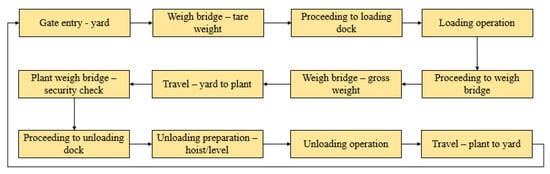
Figure A1.
Process mapping flow chart for interfacility material transfer.
Figure A1.
Process mapping flow chart for interfacility material transfer.
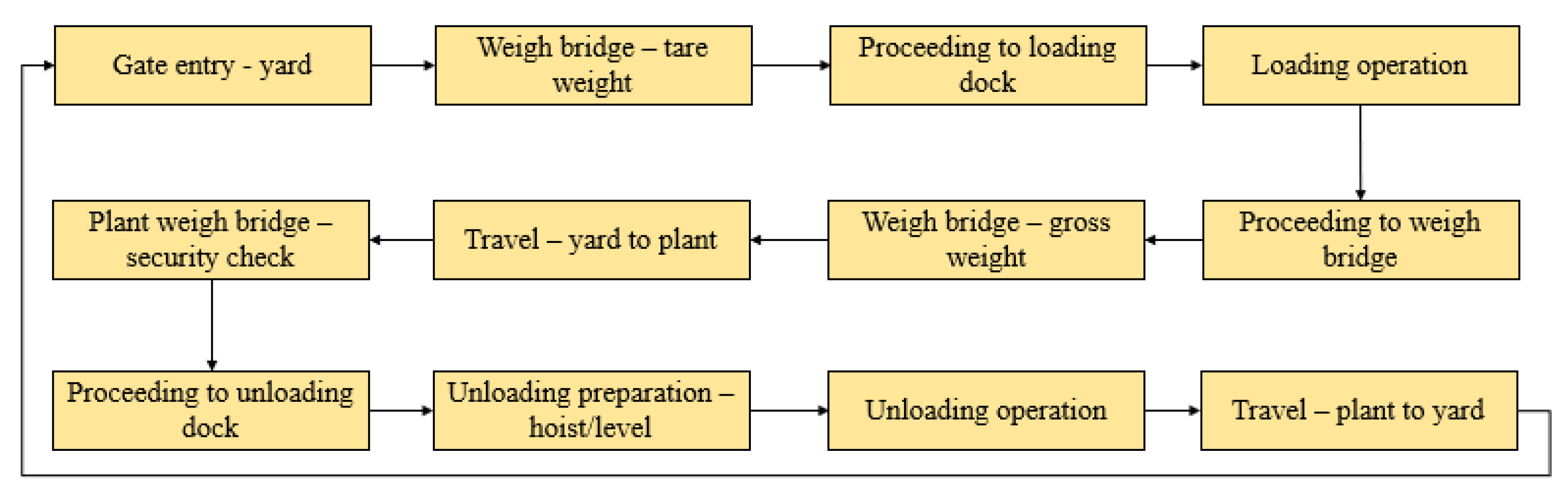

Figure A2.
Simulation optimisation run window for scenario 3; cost–time series.
Figure A2.
Simulation optimisation run window for scenario 3; cost–time series.
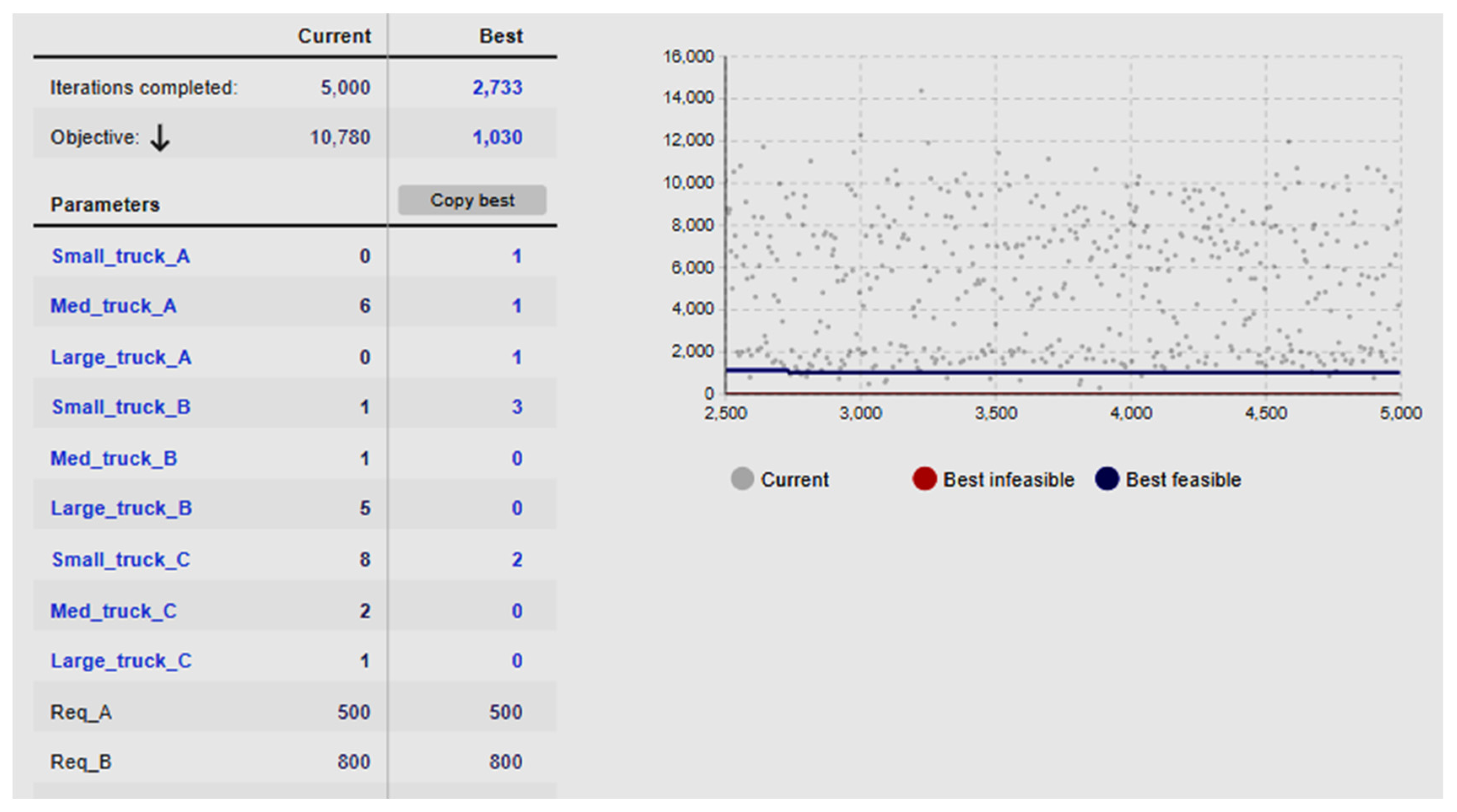
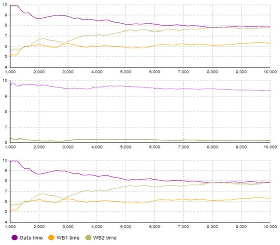
Figure A3.
Service time for product class A, B, and C for gate services, weigh bridges 1 and 2.
Figure A3.
Service time for product class A, B, and C for gate services, weigh bridges 1 and 2.
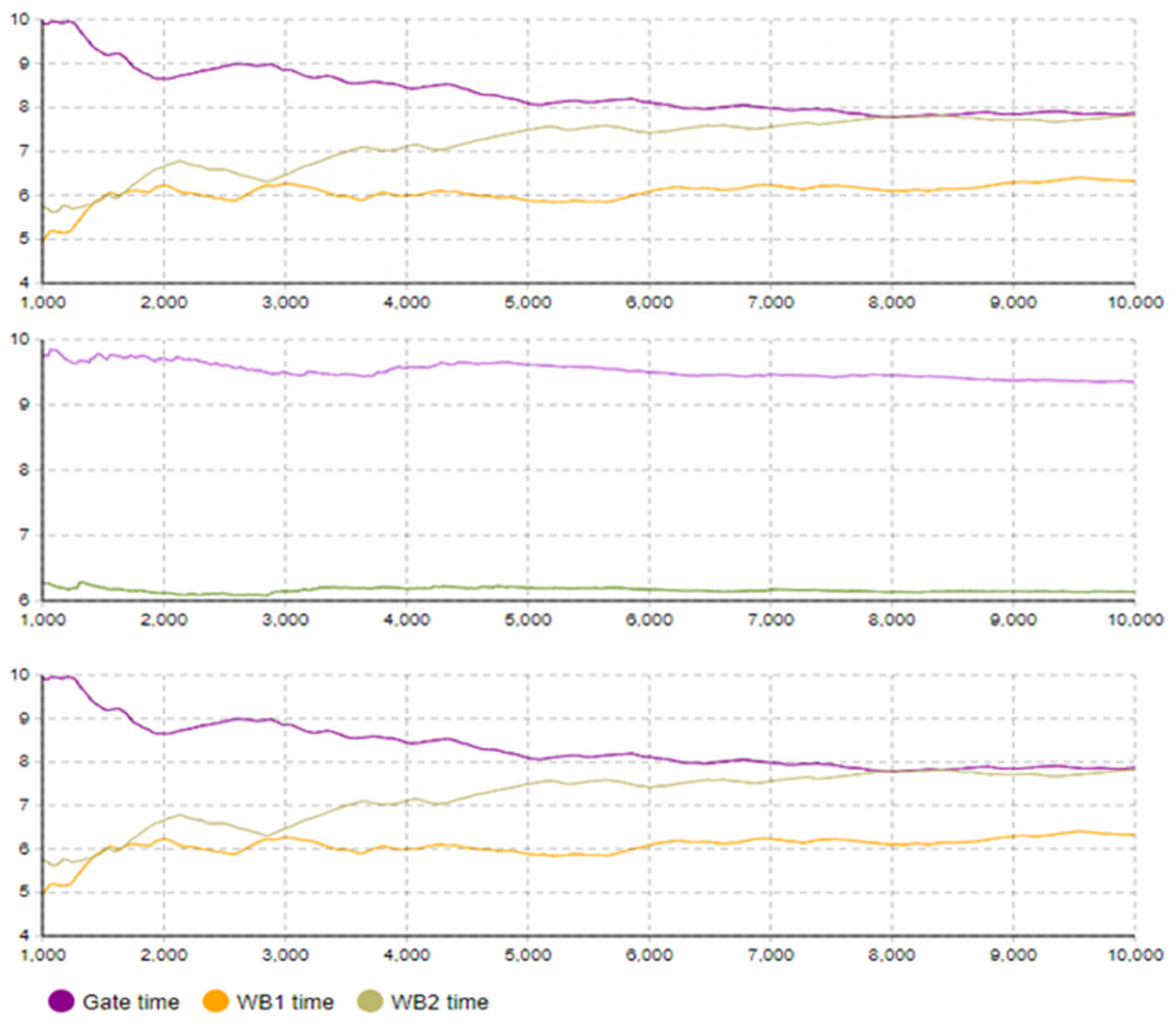
Table A1.
Node labelling details for all service stations.
Table A1.
Node labelling details for all service stations.
| Node | Detail | Node | Detail |
|---|---|---|---|
| 1 | Gate | 13 | Proceeding to loading dock–B, C |
| 2 | Weigh bridge (WB1)–tare weight | 14 | Loading operation–B |
| 3 | Proceeding to loading dock–A | 15 | Proceeding to WB2–B, C |
| 4 | Loading operation–A | 16 | Travel–yard to plant–B, C |
| 5 | Proceeding to WB | 17 | Plant WB–B, C |
| 6 | WB–gross weight | 18 | Proceeding to unloading dock–B |
| 7 | Travel–yard to plant–A | 19 | Plant to yard–B, C |
| 8 | Plant WB–A | 20 | Loading operation–C |
| 9 | Proceeding to unloading dock–A | 21 | Proceeding to unloading dock–C |
| 10 | Unloading preparation–A, B | 22 | Unloading preparation–C |
| 11 | Unloading operation–A, B | 23 | Unloading operation–C |
| 12 | Travel–plant to yard–A | - | - |
Table A2.
Process service times.
Table A2.
Process service times.
| Process | Ave. Time (min) | Process | Ave. Time (min) |
|---|---|---|---|
| Gate entry–yard | 1.5 | Travel–yard to plant–B, C | 14 |
| WB–tare weight | 1.5 | Plant WB–A | 0.45 |
| Proc. to loading dock–A | 1.5 | Plant WB–B, C | 0.45 |
| Proc. to loading dock–B, C | 1.5 | Proc. to unloading dock–A, B | 1.5 |
| * Loading–A | 6, 7, 8 | Proc. to unloading dock–C | 5 |
| * Loading–B | 12, 17, 23 | Unloading preparation | 8 |
| * Loading–C | 6, 7, 8 | * Unloading–A | 2, 2.5, 3 |
| Proceeding to WB–A | 2.5 | * Unloading–B | 2, 2.5, 3 |
| Proceeding to WB–B, C | 1.5 | * Unloading–C | 2, 2.5, 3 |
| WB–gross weight | 0.45 | Travel–plant to yard–A, B | 12 |
| Travel–yard to plant–A | 18 | Travel–plant to yard–B | 12 |
* Service times are for small, medium, and large trucks, respectively.
References
- Saez-Mas, A.; Garcia-Sabater, J.P.; Garcia-Sabater, J.J.; Ruiz, A. Redesigning the in-plant supply logistics: A case study. Comput. Ind. Eng. 2020, 143, 106422. [Google Scholar] [CrossRef]
- Funke, T.; Becker, T. Complex networks of material flow in manufacturing and logistics: Modeling, analysis, and prediction using stochastic block models. J. Manuf. Syst. 2020, 56, 296–311. [Google Scholar] [CrossRef]
- Pan, C.; Chang, Q.; Ni, J. Real time dispatching control of multi-dollies material handling systems in general assembly lines. In Proceedings of the International Manufacturing Science and Engineering Conference, Singapore, 27–28 June 2012; American Society of Mechanical Engineers: New York, NY, USA, 2012; Volume 54990, pp. 377–386. [Google Scholar]
- Emde, S.; Boysen, N. Optimally locating in-house logistics areas to facilitate JIT-supply of mixed-model assembly lines. Int. J. Prod. Econ. 2012, 135, 393–402. [Google Scholar] [CrossRef]
- Carter, C.R.; Rogers, D.S. A framework of sustainable supply chain management: Moving toward new theory. Int. J. Phys. Distrib. Logist. Manag. 2008, 38, 360–387. [Google Scholar] [CrossRef]
- Sbahieh, S.; Mckay, G.; Al-Ghamdi, S.G. A comparative life cycle assessment of fiber-reinforced polymers as a sustainable reinforcement option in concrete beams. Front. Built Environ. 2023, 9, 1194121. [Google Scholar] [CrossRef]
- Mahmood, K.; Karjust, K.; Raamets, T. Production intralogistics automation based on 3D simulation analysis. J. Mach. Eng. 2021, 21, 102–115. [Google Scholar] [CrossRef]
- Cho, C.; Egbelu, P.J. Design of a web-based integrated material handling system for manufacturing applications. Int. J. Prod. Res. 2005, 43, 375–403. [Google Scholar] [CrossRef]
- Rakhmangulov, A.; Sładkowski, A.; Osintsev, N.; Mishkurov, P.; Muravev, D. Dynamic optimization of railcar traffic volumes at railway nodes. In Rail Transport—Systems Approach; Springer: Berlin/Heidelberg, Germany, 2017; pp. 405–456. [Google Scholar]
- Marotta, A.; Studer, L.; Marchionni, G.; Ponti, M.; Gandini, P.; Agriesti, S.; Arena, M. Possible impacts of C-ITS on supply-chain logistics system. Transp. Res. Procedia 2018, 30, 332–341. [Google Scholar] [CrossRef]
- Fartaj, S.-R.; Kabir, G.; Eghujovbo, V.; Ali, S.M.; Paul, S.K. Modeling transportation disruptions in the supply chain of automotive parts manufacturing company. Int. J. Prod. Econ. 2020, 222, 107511. [Google Scholar] [CrossRef]
- Lanza, G.; Ferdows, K.; Kara, S.; Mourtzis, D.; Schuh, G.; Váncza, J.; Wang, L.; Wiendahl, H.-P. Global production networks: Design and operation. CIRP Ann. 2019, 68, 823–841. [Google Scholar] [CrossRef]
- Cantini, A. Reviewing the Configuration of Spare Parts Supply Chains Considering Stock Deployment and Manufacturing Options. 2023. Available online: https://ntnuopen.ntnu.no/ntnu-xmlui/handle/11250/3056511 (accessed on 10 November 2023).
- Fragapane, G.; de Koster, R.; Sgarbossa, F.; Strandhagen, J.O. Planning and control of autonomous mobile robots for intralogistics: Literature review and research agenda. Eur. J. Oper. Res. 2021, 294, 405–426. [Google Scholar] [CrossRef]
- Ferriol-Galmés, M.; Suárez-Varela, J.; Paillise, J.; Shi, X.; Xiao, S.; Cheng, X.; Barlet-Ros, P.; Cabellos-Aparicio, A. Building a Digital Twin for Network Optimization Using Graph Neural Networks. SSRN Electron. J. 2021, 217, 109329. [Google Scholar] [CrossRef]
- Ekren, B.Y.; Akpunar, A. An open queuing network-based tool for performance estimations in a shuttle-based storage and retrieval system. Appl. Math. Model. 2021, 89, 1678–1695. [Google Scholar] [CrossRef]
- Lamballais, T.; Merschformann, M.; Roy, D.; de Koster, M.B.M.; Azadeh, K.; Suhl, L. Dynamic policies for resource reallocation in a robotic mobile fulfillment system with time-varying demand. Eur. J. Oper. Res. 2021, 300, 937–952. [Google Scholar] [CrossRef]
- Otten, S.; Krenzler, R.; Xie, L.; Daduna, H.; Kruse, K. Analysis of semi-open queueing networks using lost customers approximation with an application to robotic mobile fulfilment systems. OR Spectr. 2021, 44, 603–648. [Google Scholar] [CrossRef]
- Wang, W.; Wu, Y.; Qi, J.; Wang, Y. Design and performance analysis of robot shuttle system. In Proceedings of the 2020 International Conference on Artificial Intelligence and Electromechanical Automation, AIEA 2020, Tianjin, China, 22–28 June 2020; pp. 255–259. [Google Scholar]
- Azadeh, K.; Roy, D.; De Koster, R. Design, modeling, and analysis of vertical robotic storage and retrieval systems. Transp. Sci. 2019, 53, 1213–1234. [Google Scholar] [CrossRef]
- Zou, B.; Xu, X.; Gong, Y.Y.; De Koster, R. Evaluating battery charging and swapping strategies in a robotic mobile fulfillment system. Eur. J. Oper. Res. 2018, 267, 733–753. [Google Scholar] [CrossRef]
- Sbahieh, S.; Rabie, M.; Ebead, U.; Al-Ghamdi, S.G. The Mechanical and Environmental Performance of Fiber-Reinforced Polymers in Concrete Structures: Opportunities, Challenges and Future Directions. Buildings 2022, 12, 1417. [Google Scholar] [CrossRef]
- Petchrompo, S.; Parlikad, A.K. A review of asset management literature on multi-asset systems. Reliab. Eng. Syst. Saf. 2019, 181, 181–201. [Google Scholar] [CrossRef]
- Amjath, M.; Kerbache, L.; Macgregor, J.; Elomri, A. Fleet sizing of trucks for an inter-facility material handling system using closed queueing networks. Oper. Res. Perspect. 2022, 9, 100245. [Google Scholar] [CrossRef]
- Baykasoğlu, A.; Subulan, K. A fuzzy-stochastic optimization model for the intermodal fleet management problem of an international transportation company. Transp. Plan. Technol. 2019, 42, 777–824. [Google Scholar] [CrossRef]
- New, C.C. Transport fleet planning for multi-period operations. J. Oper. Res. Soc. 1975, 26, 151–166. [Google Scholar] [CrossRef]
- Etezadi, T.; Beasley, J.E. Vehicle fleet composition. J. Oper. Res. Soc. 1983, 34, 87–91. [Google Scholar] [CrossRef]
- Klincewicz, J.G.; Luss, H.; Pilcher, M.G. Fleet size planning when outside carrier services are available. Transp. Sci. 1990, 24, 169–182. [Google Scholar] [CrossRef]
- Desrochers, M.; Verhoog, T.W. A new heuristic for the fleet size and mix vehicle routing problem. Comput. Oper. Res. 1991, 18, 263–274. [Google Scholar] [CrossRef]
- Couillard, J.; Martel, A. Vehicle fleet planning the road transportation industry. IEEE Trans. Eng. Manag. 1990, 37, 31–36. [Google Scholar] [CrossRef]
- Salhi, S.; Rand, G.K. Incorporating vehicle routing into the vehicle fleet composition problem. Eur. J. Oper. Res. 1993, 66, 313–330. [Google Scholar] [CrossRef]
- Liu, F.-H.; Shen, S.-Y. The fleet size and mix vehicle routing problem with time windows. J. Oper. Res. Soc. 1999, 50, 721–732. [Google Scholar] [CrossRef]
- Zhao, Q.-H.; Wang, S.-Y.; Lai, K.K.; Xia, G.-P. Dynamic multi-period transportation model for vehicle composition with transshipment points. Adv. Model. Optim. 2001, 3, 17–28. [Google Scholar]
- List, G.F.; Wood, B.; Nozick, L.K.; Turnquist, M.A.; Jones, D.A.; Kjeldgaard, E.A.; Lawton, C.R. Robust optimization for fleet planning under uncertainty. Transp. Res. Part E Logist. Transp. Rev. 2003, 39, 209–227. [Google Scholar] [CrossRef]
- Renaud, J.; Boctor, F.F. A sweep-based algorithm for the fleet size and mix vehicle routing problem. Eur. J. Oper. Res. 2002, 140, 618–628. [Google Scholar] [CrossRef]
- Papier, F.; Thonemann, U.W. Queuing models for sizing and structuring rental fleets. Transp. Sci. 2008, 42, 302–317. [Google Scholar] [CrossRef]
- Jabali, O.; Gendreau, M.; Laporte, G. A continuous approximation model for the fleet composition problem. Transp. Res. Part B Methodol. 2012, 46, 1591–1606. [Google Scholar] [CrossRef]
- Redmer, A.; Żak, J.; Sawicki, P.; Maciejewski, M. Heuristic approach to fleet composition problem. Procedia-Soc. Behav. Sci. 2012, 54, 414–427. [Google Scholar] [CrossRef]
- Zak, J.; Redmer, A.; Sawicki, P. Multiple objective optimization of the fleet sizing problem for road freight transportation. J. Adv. Transp. 2008, 42, 379–427. [Google Scholar] [CrossRef]
- Roy, D.; Sebastian, J.; Sharma, D. Fleet sizing for transporters with seasonal demands. Int. J. Autom. Logist. 2013, 1, 105–115. [Google Scholar] [CrossRef]
- Meghjani, M.; Pendleton, S.D.; Marczuk, K.A.; Eng, Y.H.; Shen, X.; Ang, M.H.; Rus, D. Multi-class fleet sizing and mobility on demand service. Adv. Intell. Syst. Comput. 2019, 878, 37–49. [Google Scholar] [CrossRef]
- Cruz, R.; Bergsten Mendes, A.; Bahiense, L.; Wu, Y. Integrating berth allocation decisions in a fleet composition and periodic routing problem of platform supply vessels. Eur. J. Oper. Res. 2019, 275, 334–346. [Google Scholar] [CrossRef]
- Vieira, B.S.; Ribeiro, G.M.; Bahiense, L.; Cruz, R.; Mendes, A.B.; Laporte, G. Exact and heuristic algorithms for the fleet composition and periodic routing problem of offshore supply vessels with berth allocation decisions. Eur. J. Oper. Res. 2021, 295, 908–923. [Google Scholar] [CrossRef]
- Fan, Q.; Van Essen, J.T.; Correia, G.H.A. Heterogeneous fleet sizing for on-demand transport in mixed automated and non-automated urban areas. Transp. Res. Procedia 2022, 62, 163–170. [Google Scholar] [CrossRef]
- Zhao, Y.; Zeng, T.; Allybokus, Z.; Guo, Y.; Moura, S. Joint Design for Electric Fleet Operator and Charging Service Provider: Understanding the Non-Cooperative Nature. IEEE Trans. Intell. Transp. Syst. 2022, 24, 115–127. [Google Scholar] [CrossRef]
- George, D.K.; Xia, C.H. Fleet-sizing and service availability for a vehicle rental system via closed queueing networks. Eur. J. Oper. Res. 2011, 211, 198–207. [Google Scholar] [CrossRef]
- Hu, L.; Liu, Y. Joint design of parking capacities and fleet size for one-way station-based carsharing systems with road congestion constraints. Transp. Res. Part B Methodol. 2016, 93, 268–299. [Google Scholar] [CrossRef]
- Bazan, P.; Djanatliev, A.; Pruckner, M.; German, R.; Lauer, C. Rebalancing and fleet sizing of mobility-on-demand networks with combined simulation, optimization and queueing network analysis. In Proceedings of the Proceedings—Winter Simulation Conference, National Harbor, MD, USA, 8–11 December 2019; Volume 2018, pp. 1527–1538. [Google Scholar]
- Iglesias, R.; Rossi, F.; Zhang, R.; Pavone, M. A BCMP network approach to modeling and controlling autonomous mobility-on-demand systems. Int. J. Rob. Res. 2019, 38, 357–374. [Google Scholar] [CrossRef]
- Kim, C.; Dudin, S.; Dudina, O. Queueing network with moving servers as a model of car sharing systems. Mathematics 2019, 7, 825. [Google Scholar] [CrossRef]
- Benjaafar, S.; Wu, S.; Liu, H.; Gunnarsson, E.B. Dimensioning On-Demand Vehicle Sharing Systems. Manag. Sci. 2022, 68, 1218–1232. [Google Scholar] [CrossRef]
- Fanti, M.P.; Mangini, A.M.; Pedroncelli, G.; Ukovich, W. Fleet sizing for electric car sharing system via closed queueing networks. In Proceedings of the Conference Proceedings—IEEE International Conference on Systems, Man and Cybernetics, San Diego, CA, USA, 5–8 October 2014; Volume 2014, pp. 1324–1329. [Google Scholar]
- Fanti, M.P.; Mangini, A.M.; Pedroncelli, G.; Ukovich, W. Fleet Sizing for Electric Car Sharing Systems in Discrete Event System Frameworks. IEEE Trans. Syst. Man Cybern. Syst. 2020, 50, 1161–1177. [Google Scholar] [CrossRef]
- Deng, Y.; Gupta, A.; Shroff, N.B. Fleet sizing and charger allocation in electric vehicle sharing systems. IFAC J. Syst. Control 2022, 22, 100210. [Google Scholar] [CrossRef]
- Samet, B.; Couffin, F.; Zolghadri, M.; Barkallah, M.; Haddar, M. Performance analysis and improvement of the bike sharing system using closed Queuing Networks with Blocking Mechanism. Sustainability 2018, 10, 4663. [Google Scholar] [CrossRef]
- Maleki Vishkaei, B.; Mahdavi, I.; Mahdavi-Amiri, N.; Khorram, E. Balancing public bicycle sharing system using inventory critical levels in queuing network. Comput. Ind. Eng. 2020, 141, 106277. [Google Scholar] [CrossRef]
- Liu, Y.; Ouyang, Y. Mobility service design via joint optimization of transit networks and demand-responsive services. Transp. Res. Part B Methodol. 2021, 151, 22–41. [Google Scholar] [CrossRef]
- Heragu, S.S.; Cai, X.; Krishnamurthy, A.; Malmborg, C.J. Analytical models for analysis of automated warehouse material handling systems. Int. J. Prod. Res. 2011, 49, 6833–6861. [Google Scholar] [CrossRef]
- Marchet, G.; Melacini, M.; Perotti, S.; Tappia, E. Analytical model to estimate performances of autonomous vehicle storage and retrieval systems for product totes. Int. J. Prod. Res. 2012, 50, 7134–7148. [Google Scholar] [CrossRef]
- Roy, D.; Krishnamurthy, A.; Heragu, S.S.; Malmborg, C.J. Performance analysis and design trade-offs in warehouses with autonomous vehicle technology. IIE Trans. Inst. Ind. Eng. 2012, 44, 1045–1060. [Google Scholar] [CrossRef]
- Roy, D.; Krishnamurthy, A.; Heragu, S.S.; Malmborg, C.J. Blocking effects in warehouse systems with autonomous vehicles. IEEE Trans. Autom. Sci. Eng. 2014, 11, 439–451. [Google Scholar] [CrossRef]
- Seyedhoseini, S.M.; Rashid, R.; Teimoury, E. Developing a cross-docking network design model under uncertain environment. J. Ind. Eng. Int. 2015, 11, 225–236. [Google Scholar] [CrossRef]
- Xu, Y.; Chen, Q.; Mao, N. System performance analysis of flexible flow shop with material handling unit. Jisuanji Jicheng Zhizao Xitong Comput. Integr. Manuf. Syst. CIMS 2016, 22, 764–773. [Google Scholar] [CrossRef]
- Roy, D.; Krishnamurthy, A.; Heragu, S.; Malmborg, C. Stochastic models for unit-load operations in warehouse systems with autonomous vehicles. Ann. Oper. Res. 2015, 231, 129–155. [Google Scholar] [CrossRef]
- Roy, D.; Krishnamurthy, A.; Heragu, S.; Malmborg, C. Queuing models to analyze dwell-point and cross-aisle location in autonomous vehicle-based warehouse systems. Eur. J. Oper. Res. 2015, 242, 72–87. [Google Scholar] [CrossRef]
- Govind, N.; Roeder, T.M.; Schruben, L.W. A simulation-based closed queueing network approximation of semiconductor automated material handling systems. IEEE Trans. Semicond. Manuf. 2011, 24, 5–13. [Google Scholar] [CrossRef]
- Nazzal, D. A closed queueing network approach to analyzing multi-vehicle material handling systems. IIE Trans. Inst. Ind. Eng. 2011, 43, 721–738. [Google Scholar] [CrossRef]
- Schleyer, M.; Gue, K. Throughput time distribution analysis for a one-block warehouse. Transp. Res. Part E Logist. Transp. Rev. 2012, 48, 652–666. [Google Scholar] [CrossRef]
- Ekren, B.Y.; Heragu, S.S.; Krishnamurthy, A.; Malmborg, C.J. Matrix-geometric solution for semi-open queuing network model of autonomous vehicle storage and retrieval system. Comput. Ind. Eng. 2014, 68, 78–86. [Google Scholar] [CrossRef]
- Liao, Y.; Chen, Q.; Mao, N.; Yu, A.; Li, X. Modelling and analysis of queueing network in flexible flow shop with non-equivalent parallel AGVs. Jisuanji Jicheng Zhizao Xitong Comput. Integr. Manuf. Syst. CIMS 2017, 23, 1950–1961. [Google Scholar] [CrossRef]
- Zhang, H.-Y.; Xi, S.-H.; Chen, Q.-X.; Smith, J.M.; Mao, N.; Li, X. Performance analysis of a flexible flow shop with random and state-dependent batch transport. Int. J. Prod. Res. 2021, 59, 982–1002. [Google Scholar] [CrossRef]
- Chen, C.; Zhao, S.X. Modeling and simulation analyses of healthcare delivery operations for inter-hospital patient transfers. In Healthcare Ethics and Training: Concepts, Methodologies, Tools, and Applications; Queen’s University: Kingston, ON, Canada; IGI Global: Hershey, PA, USA, 2017; Volume 1, pp. 241–259. [Google Scholar]
- Chen, W.; Wang, Z.; Chan, F.T.S. Robust production capacity planning under uncertain wafer lots transfer probabilities for semiconductor automated material handling systems. Eur. J. Oper. Res. 2017, 261, 929–940. [Google Scholar] [CrossRef]
- Motaghedi-Larijani, A.; Aminnayeri, M. Optimizing the admission time of outbound trucks entering a cross-dock with uniform arrival time by considering a queuing model. Eng. Optim. 2017, 49, 466–480. [Google Scholar] [CrossRef]
- Tappia, E.; Roy, D.; Melacini, M.; De Koster, R. Integrated storage-order picking systems: Technology, performance models, and design insights. Eur. J. Oper. Res. 2019, 274, 947–965. [Google Scholar] [CrossRef]
- Mohammadi, M.; Dauzère-pérès, S.; Yugma, C.; Karimi-Mamaghan, M. A queue-based aggregation approach for performance evaluation of a production system with an AMHS. Comput. Oper. Res. 2020, 115, 104838. [Google Scholar] [CrossRef]
- Choobineh, F.F.; Asef-Vaziri, A.; Huang, X. Fleet sizing of automated guided vehicles: A linear programming approach based on closed queuing networks. Int. J. Prod. Res. 2012, 50, 3222–3235. [Google Scholar] [CrossRef]
- Pascual, R.; Martínez, A.; Giesen, R. Joint optimization of fleet size and maintenance capacity in a fork-join cyclical transportation system. J. Oper. Res. Soc. 2013, 64, 982–994. [Google Scholar] [CrossRef]
- Yuan, Z.; Gong, Y. Improving the Speed Delivery for Robotic Warehouses. IFAC-Pap. 2016, 49, 1164–1168. [Google Scholar]
- Munoz, F.; Lee, S. A stochastic model to determine the required number of trucks in sugarcane harvest systems. In Proceedings of the IISE Annual Conference and Expo, Online, 22–25 May 2021; pp. 704–709. Available online: https://www.scopus.com/inward/record.uri?eid=2-s2.0-85120964379&partnerID=40&md5=8e1993dedb3dff74e5557c911bc4f5bb (accessed on 12 February 2023).
- Amjath, M.; Kerbache, L.; Elomri, A.; Smith, J.M. Fleet sizing of heterogeneous fleet of trucks in a material handling system using anylogic simulation modelling. In Proceedings of the 5th European International Conference on Industrial Engineering and Operations Management, Rome, Italy, 26–28 July 2022. [Google Scholar]
- Rouzafzoon, J. Development of Transportation and Supply Chain Problems with the Combination of Agent-Based Simulation and Network Optimization. 2023. Available online: https://osuva.uwasa.fi/bitstream/handle/10024/15296/978-952-395-067-2.pdf?sequence=2 (accessed on 12 February 2023).
- Bebortta, S.; Tripathy, S.S.; Modibbo, U.M.; Ali, I. An optimal fog-cloud offloading framework for big data optimization in heterogeneous IoT networks. Decis. Anal. J. 2023, 8, 100295. [Google Scholar] [CrossRef]
- Suri, R.; Sahu, S.; Vernon, M. Approximate mean value analysis for closed queuing networks with multiple-server stations. In Proceedings of the IIE Annual Conference Expo 2007—Industrial Engineering’s Critical Role in a Flat World—Conference Proceedings, MAdison, WI, USA, 19–23 May 2007; pp. 1618–1623. [Google Scholar]
- Reiser, M.; Lavenberg, S.S. Mean-value analysis of closed multichain queuing networks. J. ACM 1980, 27, 313–322. [Google Scholar] [CrossRef]
- Papadimitriou, C.H.; Tsitsiklis, J.N. The complexity of optimal queueing network control. In Proceedings of the IEEE 9th Annual Conference on Structure in Complexity Theory, Amsterdam, The Netherlands, 28 June–1 July 1994; IEEE: New York, NY, USA, 1994; pp. 318–322. [Google Scholar]
- Schittkowski, K. Nlpql: A fortran subroutine solving constrained nonlinear programming problems. Ann. Oper. Res. 1986, 5, 485–500. [Google Scholar] [CrossRef]

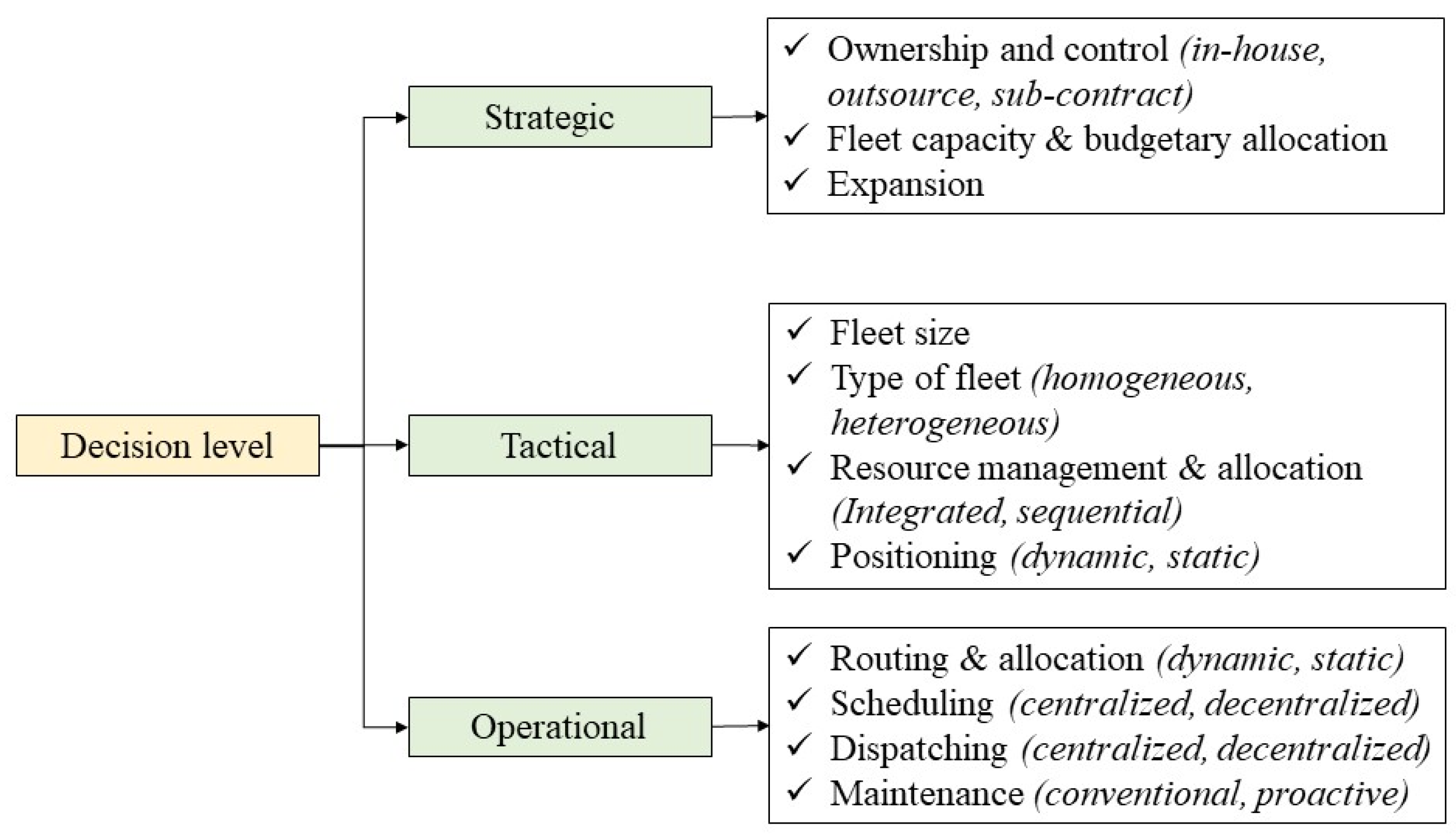
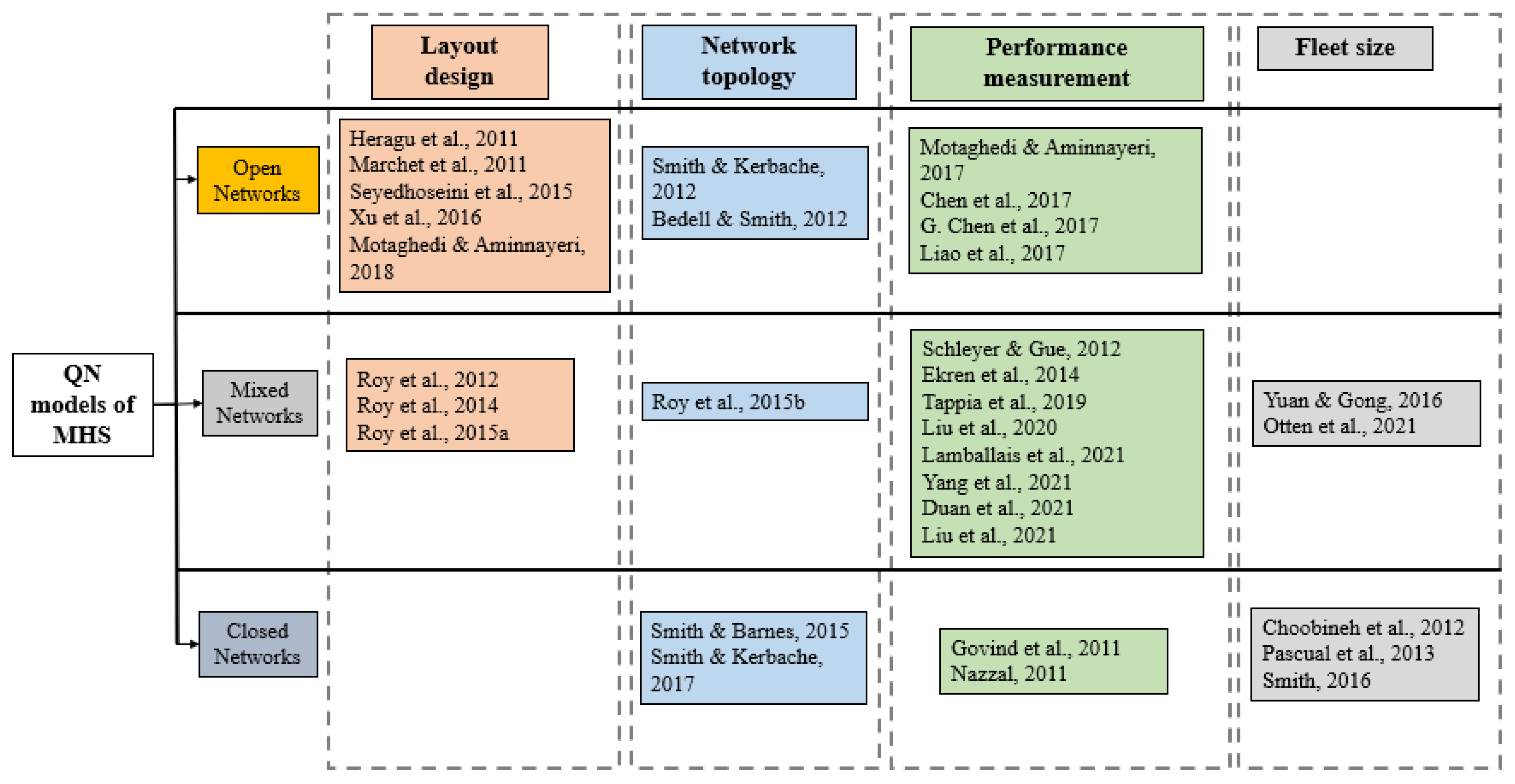
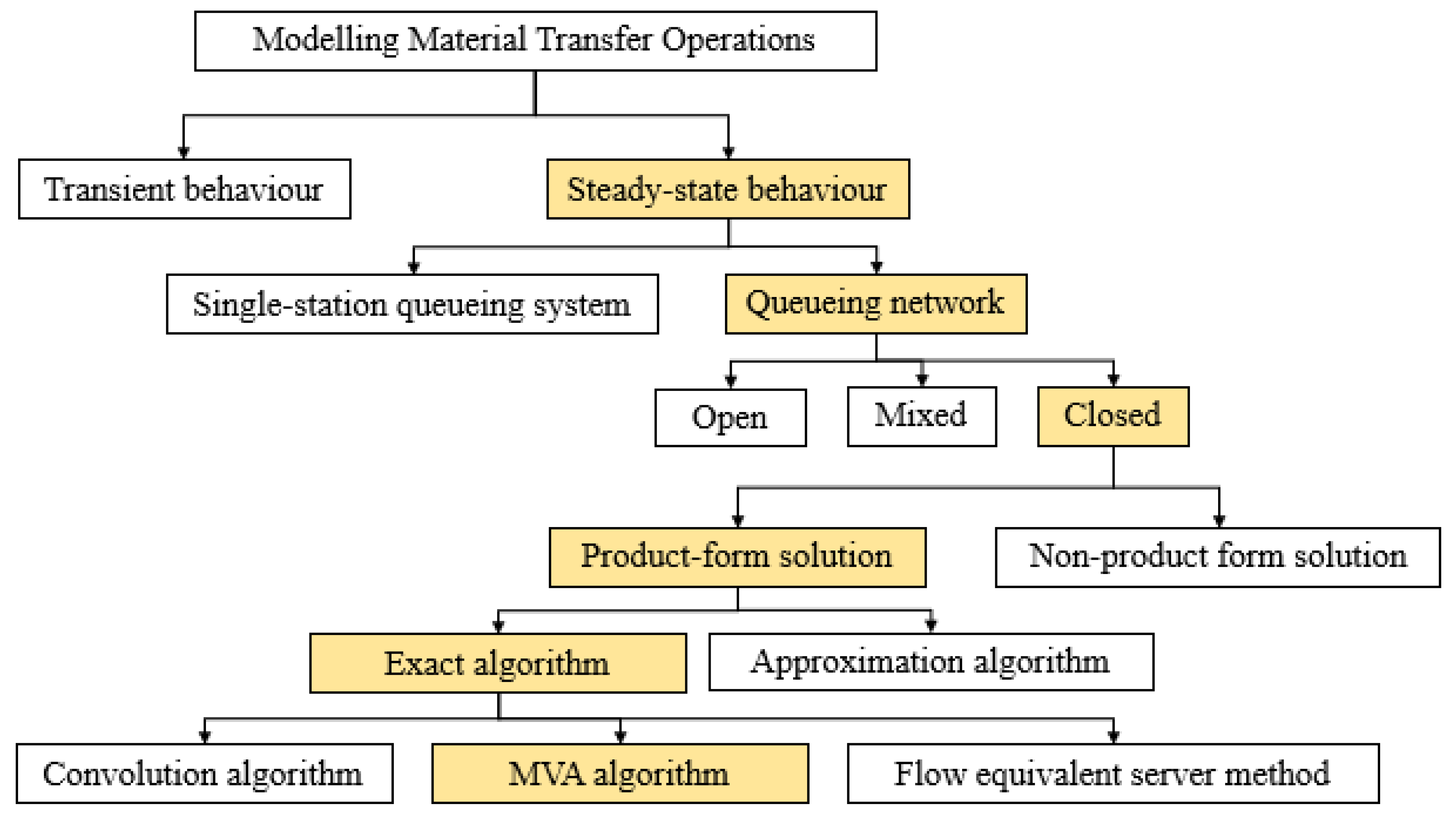
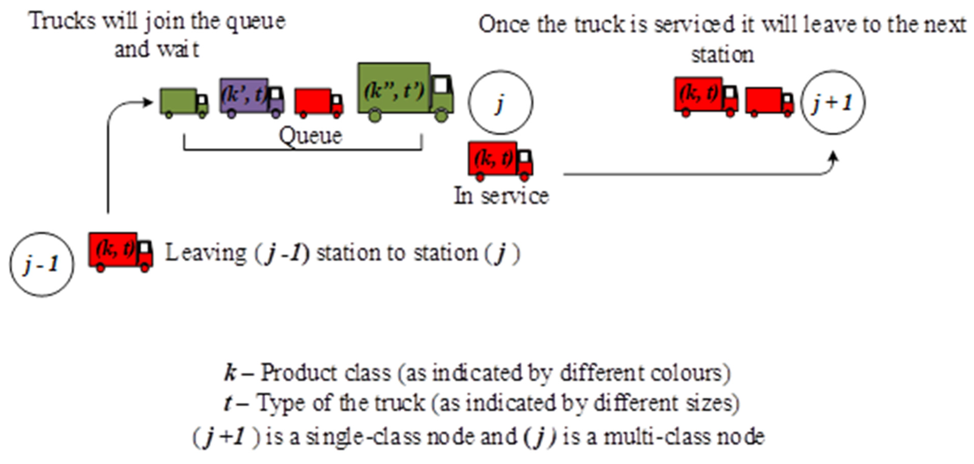

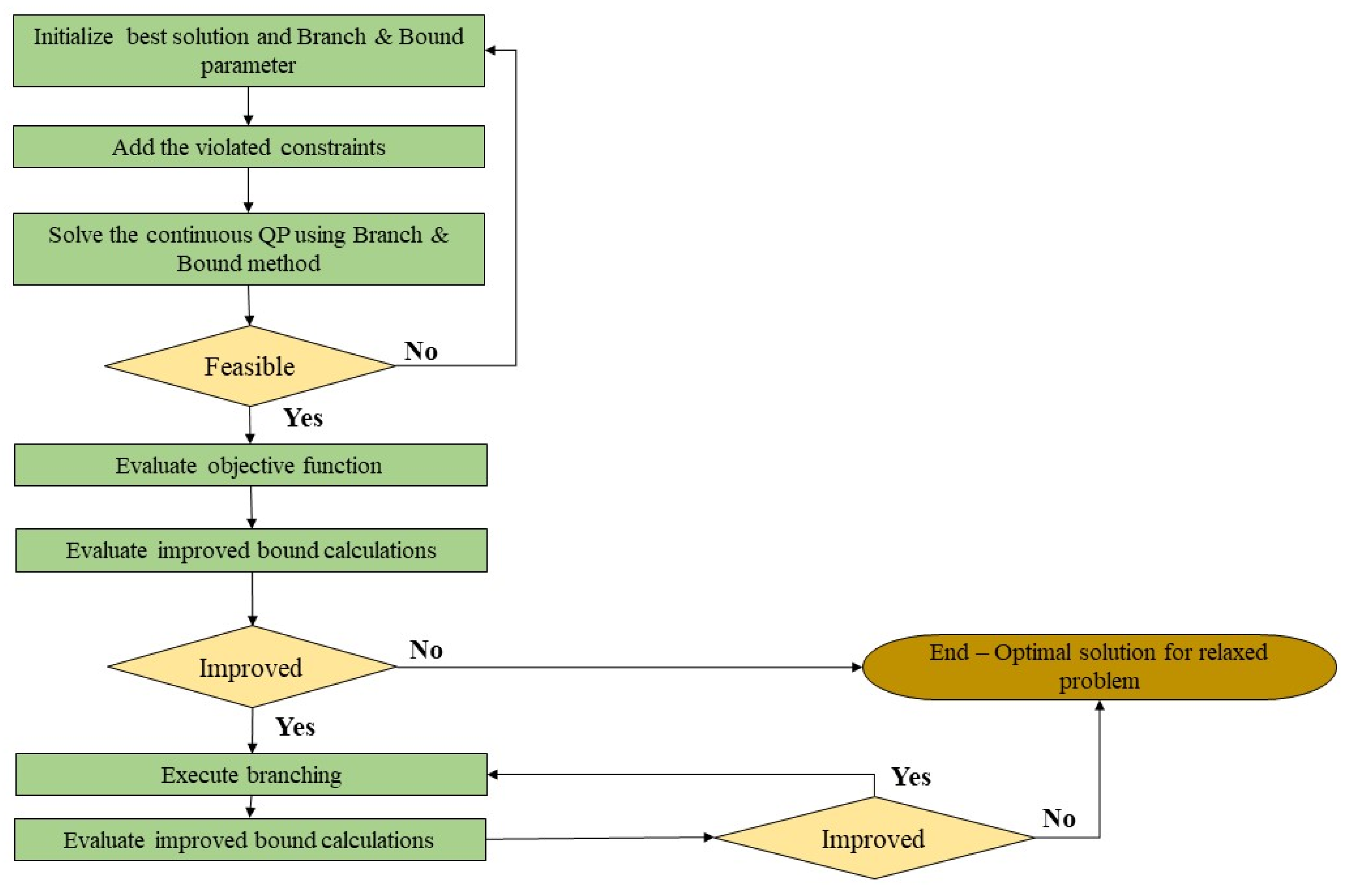

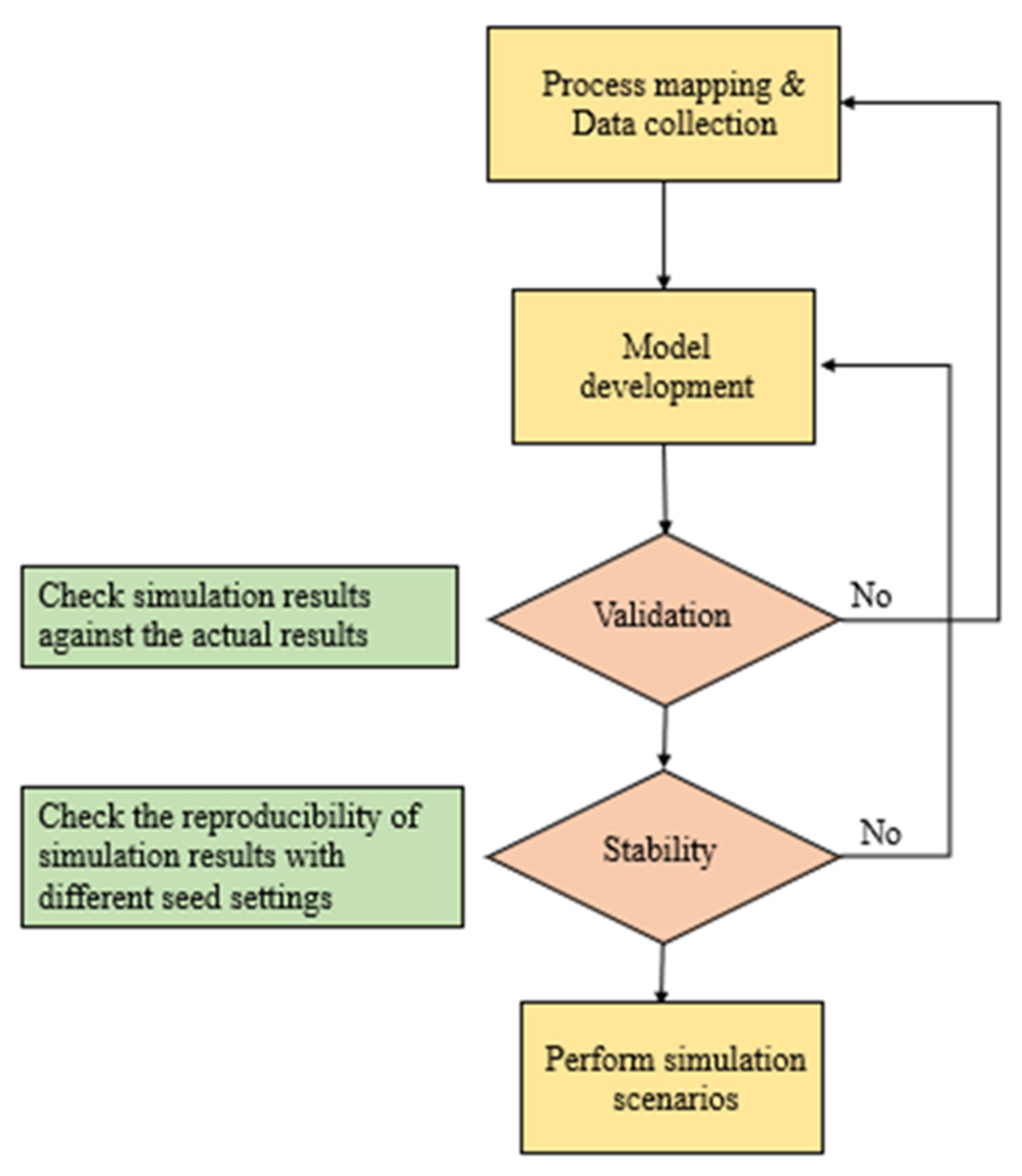
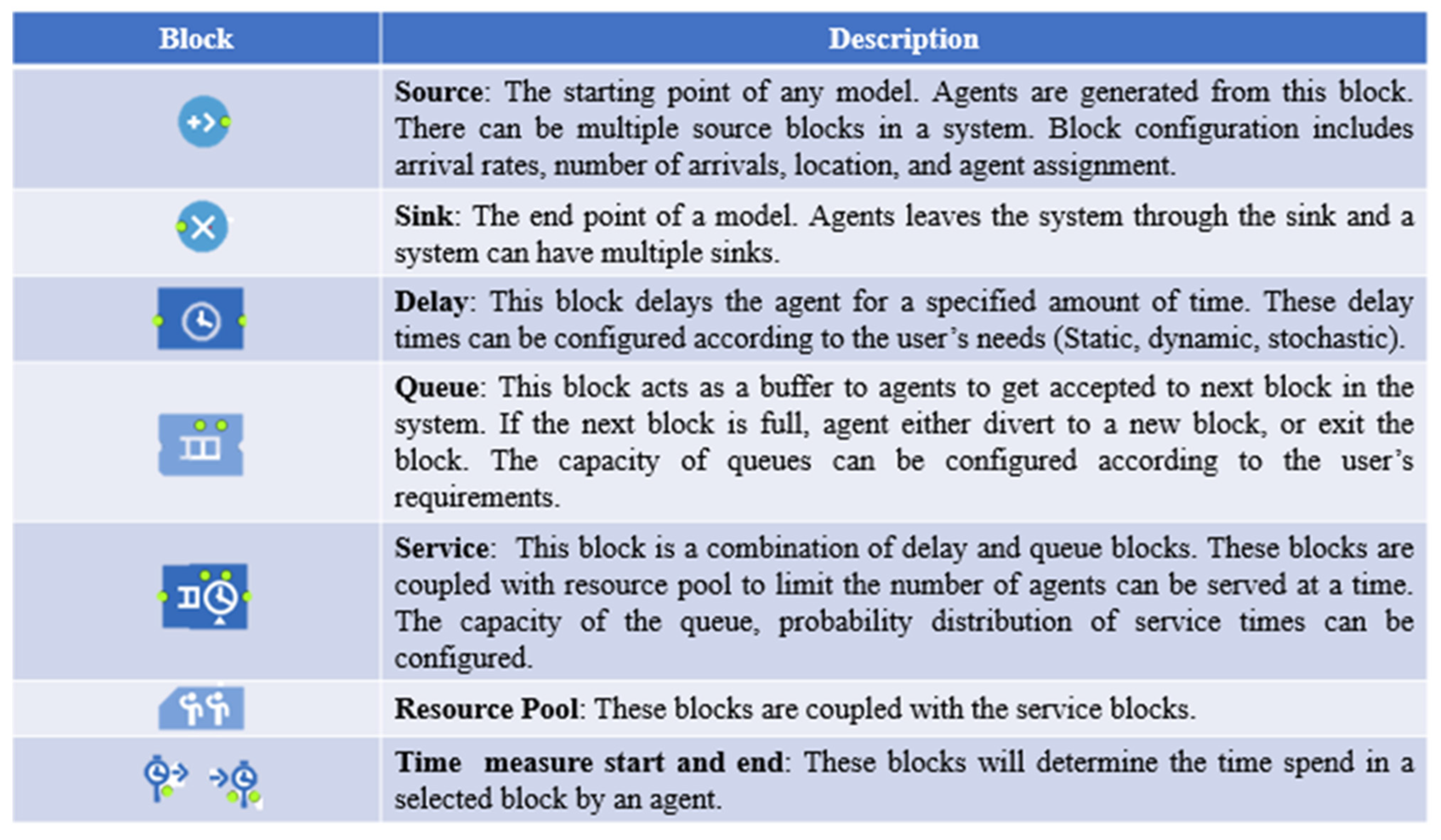
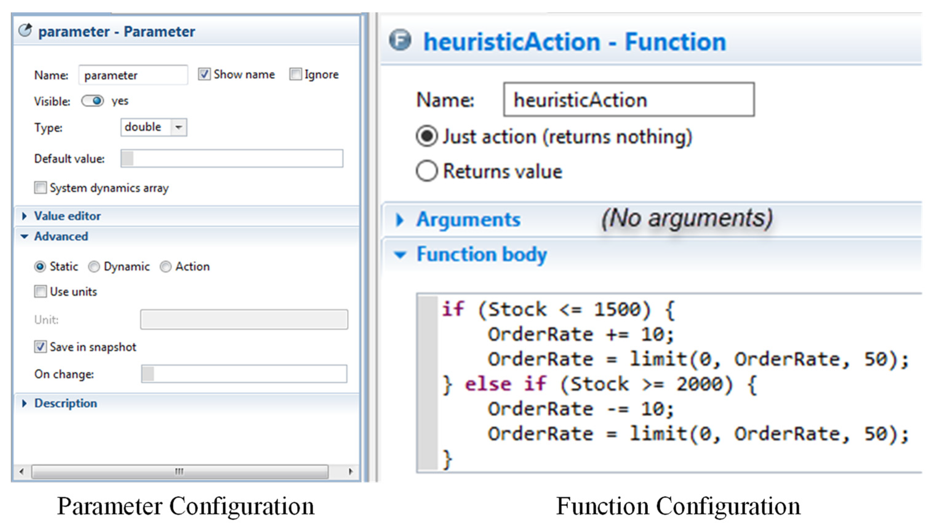
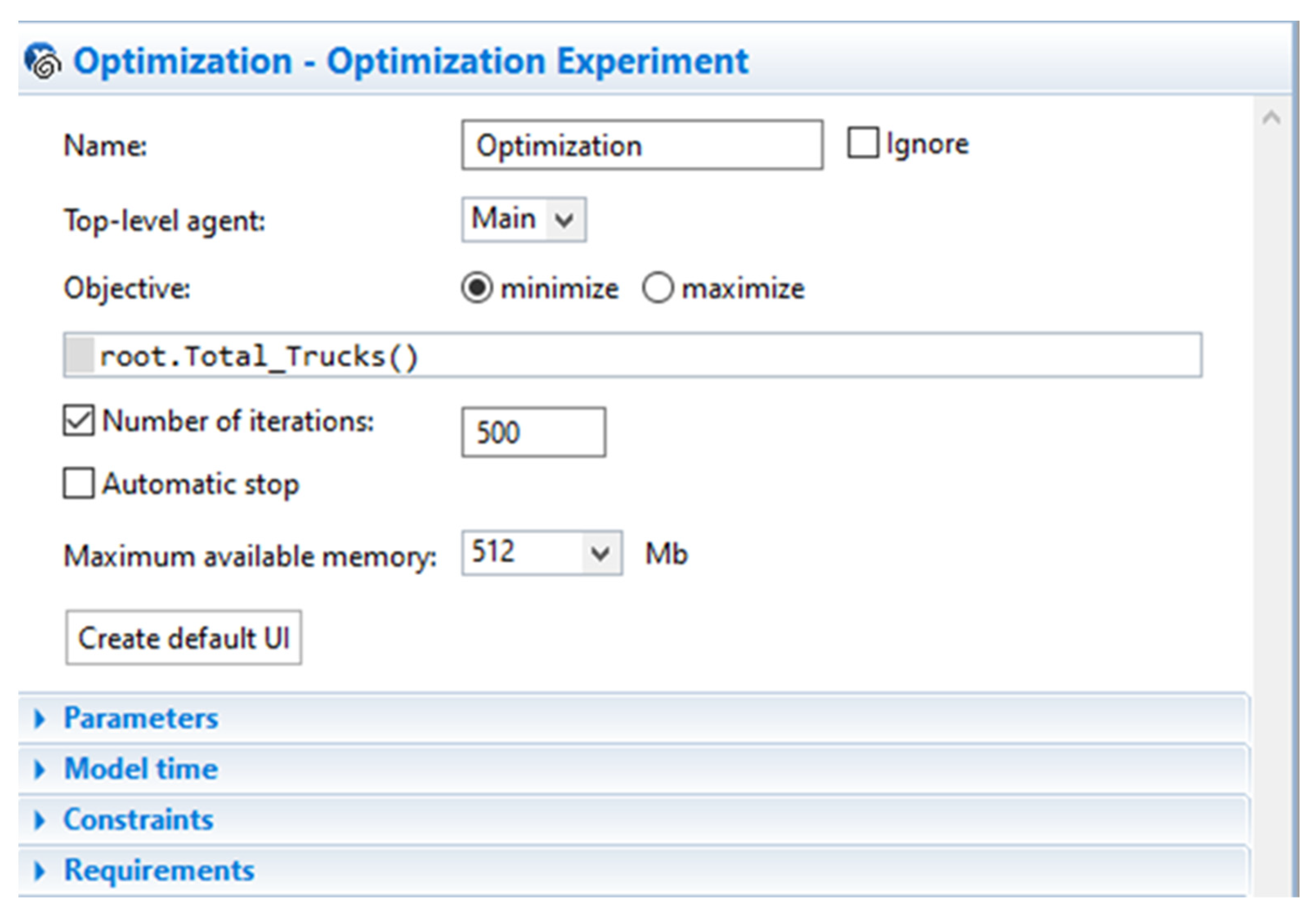
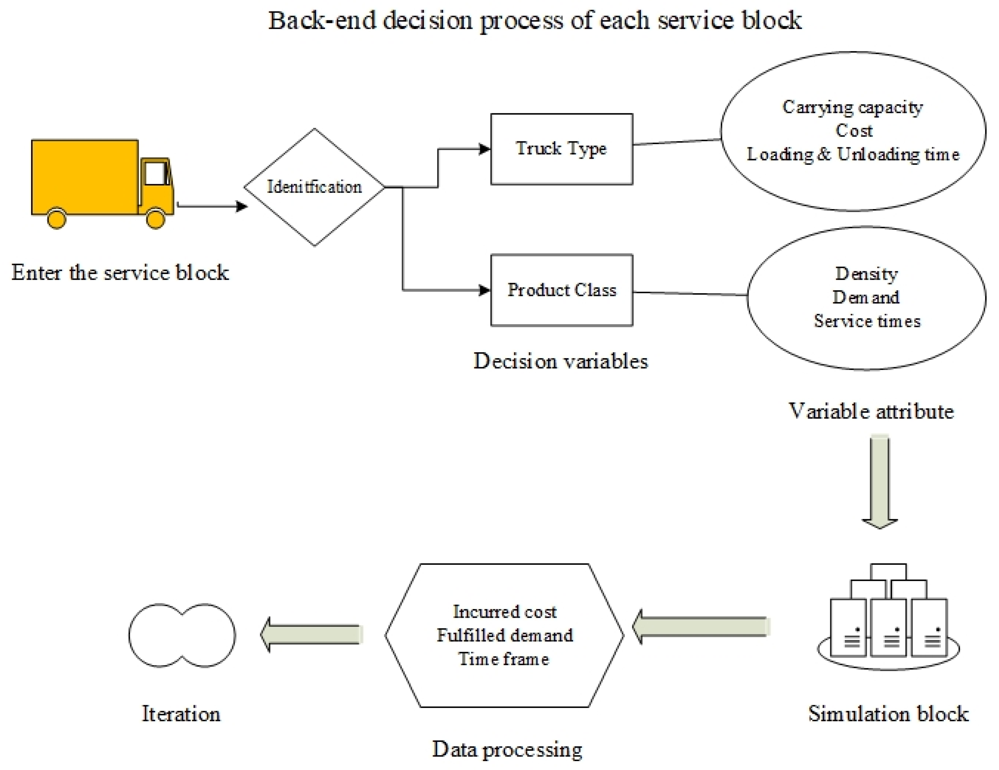
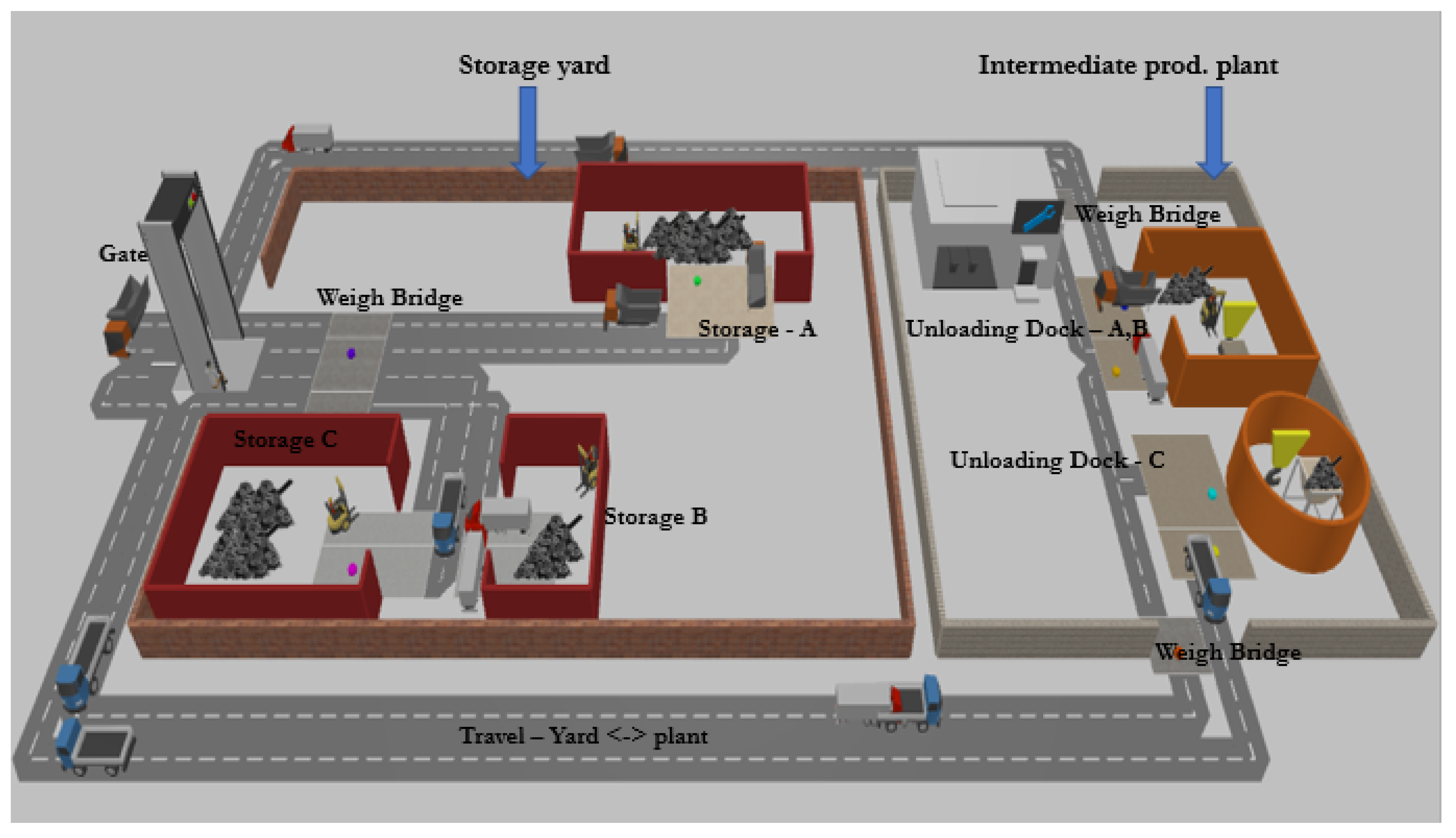
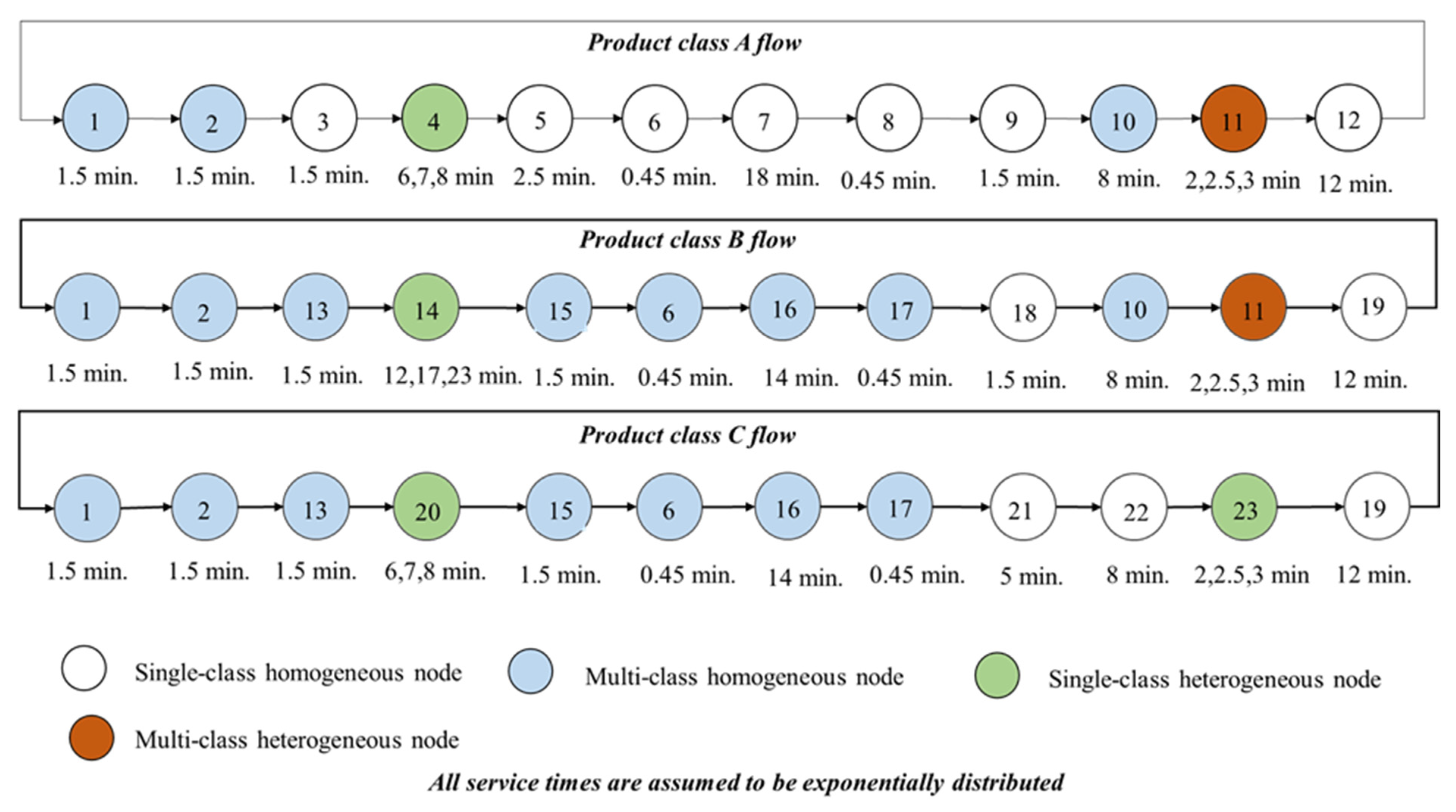
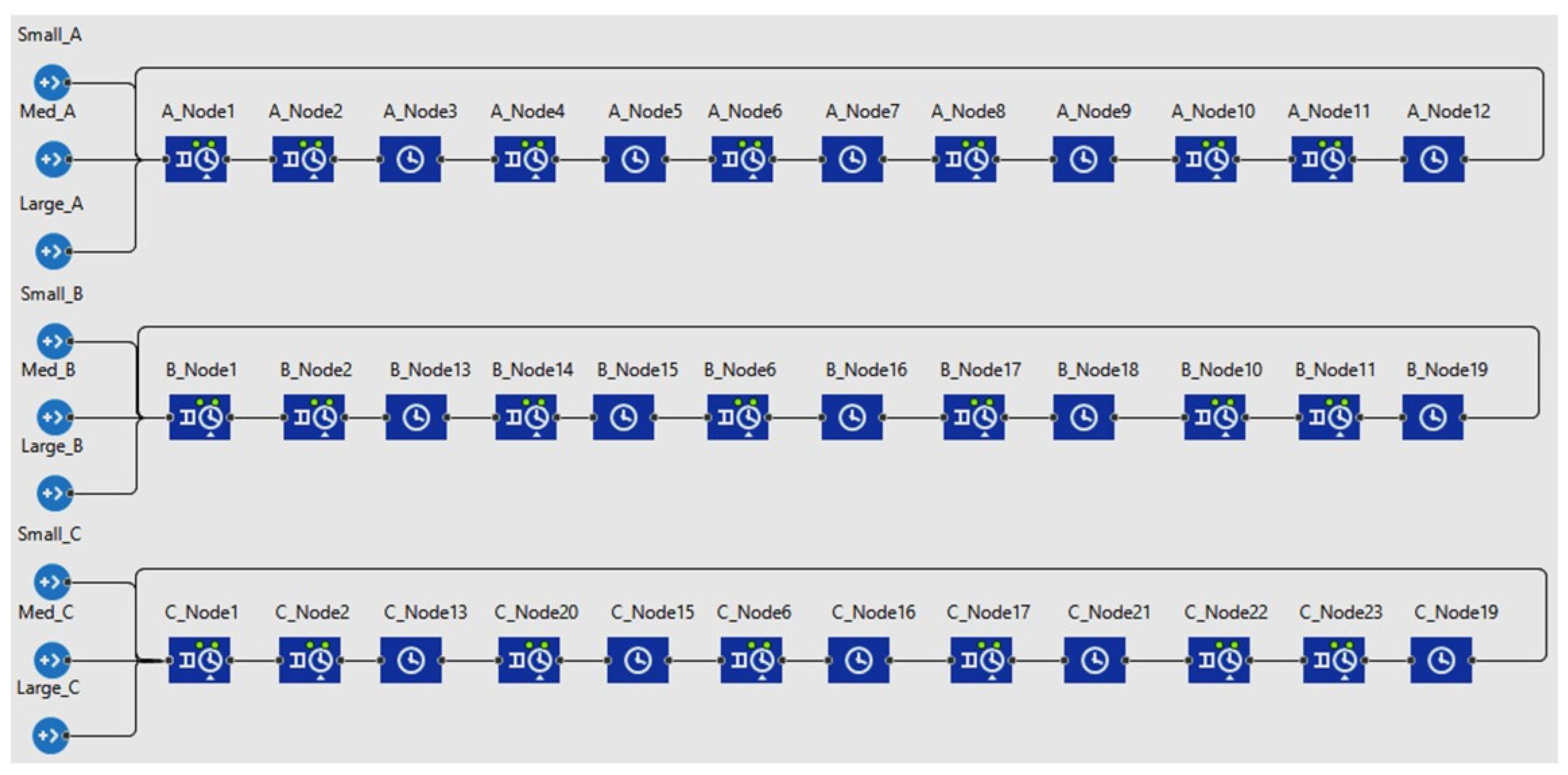
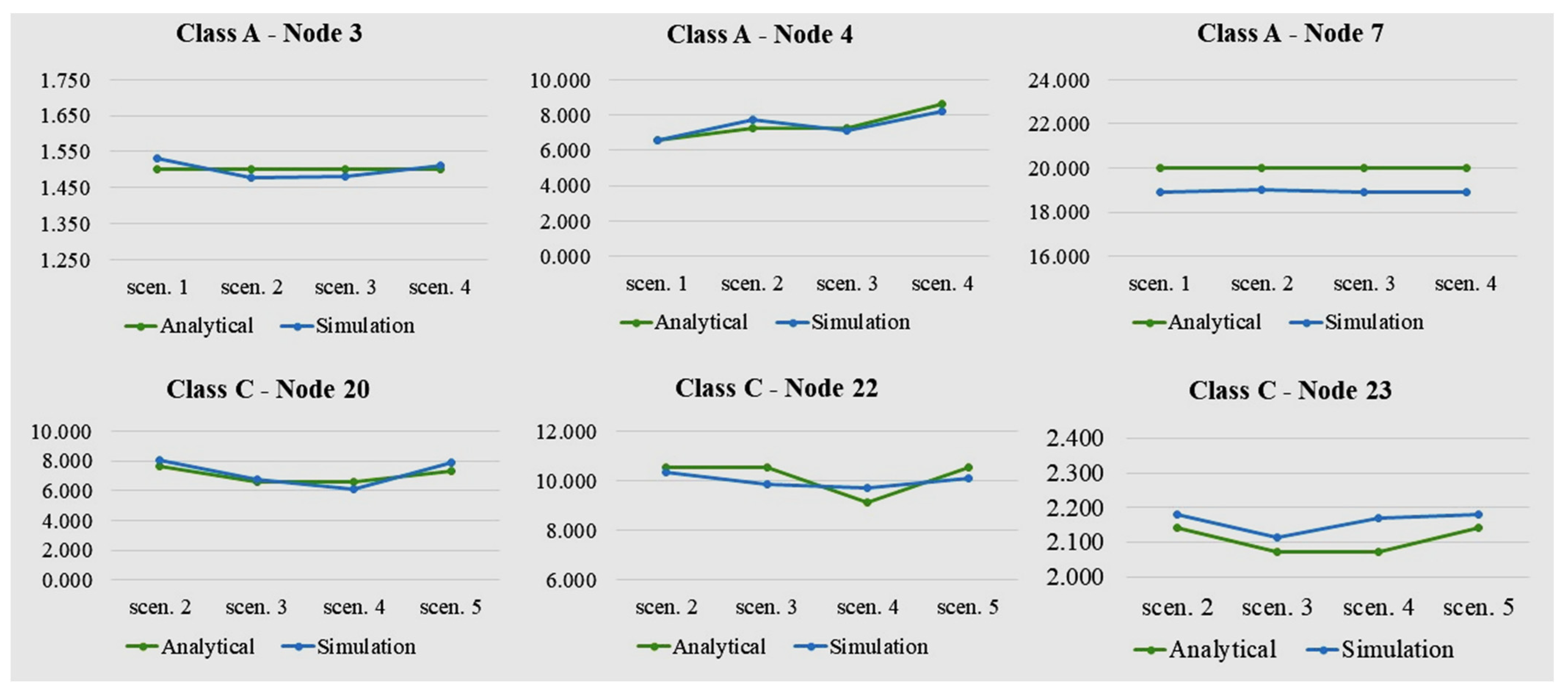
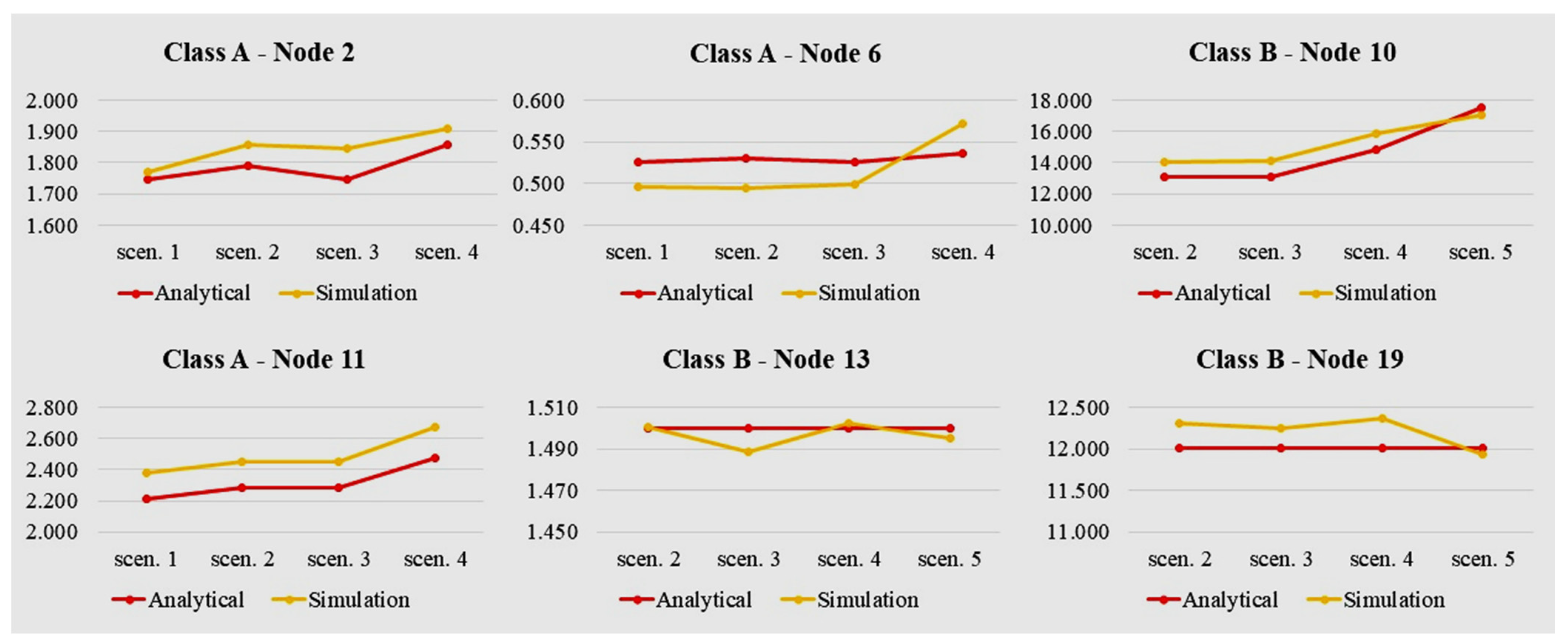

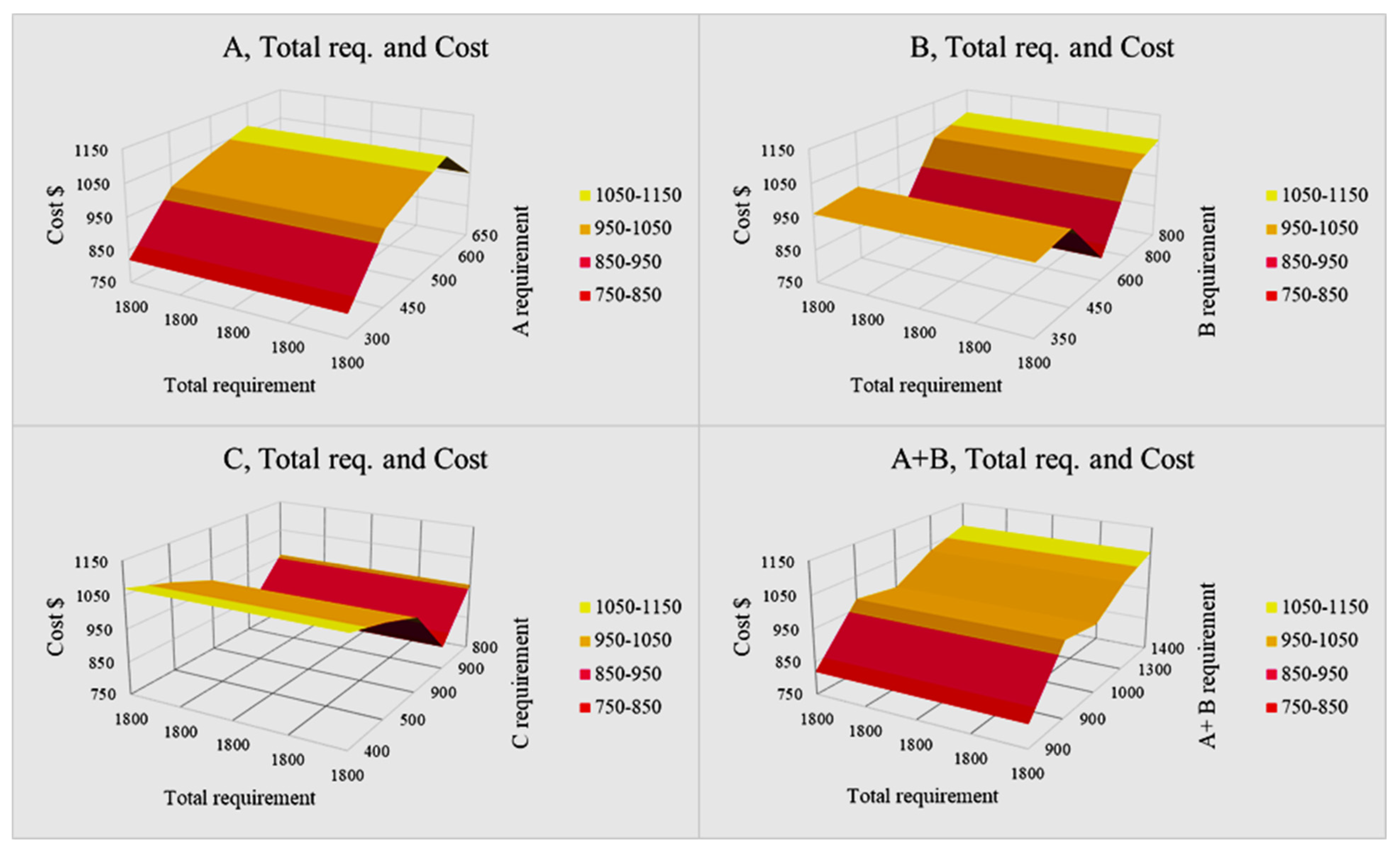
Disclaimer/Publisher’s Note: The statements, opinions and data contained in all publications are solely those of the individual author(s) and contributor(s) and not of MDPI and/or the editor(s). MDPI and/or the editor(s) disclaim responsibility for any injury to people or property resulting from any ideas, methods, instructions or products referred to in the content. |
© 2024 by the authors. Licensee MDPI, Basel, Switzerland. This article is an open access article distributed under the terms and conditions of the Creative Commons Attribution (CC BY) license (https://creativecommons.org/licenses/by/4.0/).