A Multi-Objective Model for Designing a Sustainable Closed-Loop Supply Chain Logistics Network

Abstract

Background: The growing concern for environmental and social issues has led to a focus on designing sustainable supply chains and increasing industrial responsibility towards society. In this paper, a multi-objective mixed-integer programming model is presented for designing a sustainable closed-loop supply chain. The model is aimed at the minimization of the total cost with the total used facilities, the negative environmental impacts, and the maximization of the positive social impacts. Methods: The epsilon-constraint method is utilized for solving the model and further extracting the Pareto solutions. Results: The result of the research clearly shows an optimal trade-off between the conflicting objectives, where, by paying more attention to the social and environmental aspects of sustainability, the total costs are increased or by optimizing the number of facilities, a better balance between the dynamics associated with the short-term and long-term goals is reached. The results of the sensitivity analysis also show that increasing the demand of the supply chain has the greatest impact on the supply chain costs compared to other objectives. Conclusions: Consequently, investigating such comprehensive sustainable objectives provides better insights into the impact of design variables on the expectations of stakeholders.

1. Introduction

The increase in customer pressure for timely and quality products, as well as the increase in global competition, has forced the organizations involved in the production of products and services to have an integrated and coordinated supply chain network. However, with the increase in the negative effects of industrial activities on the environment and the increase in awareness of its impacts, as well as the pressure of legislator institutions, the traditional supply chain has been pushed towards the green supply chain (GSC). In fact, the GSC concentrates on eco-friendly aspects of the supply chain operations to bring the greenness concept to all processes throughout the supply chain including product design, raw material sourcing, manufacturing and distribution processes, etc. It can be seen recently that corporate pressures on organizations, such as the need to assess the viability of vendors and employees, has put forward a broader concept of the supply chain as sustainable supply chain management (SSCM). SSCM amounts to the economic, environmental, and social consequences of the supply chain operation, known as the triple bottom of sustainability. SSCM measures make the supply chain accountable to public and social concerns such as the social and ethical issues around strategic procurement.

Today, due to the increasing attention to social and environmental issues, reverse logistics has become an important strategy to increase customer satisfaction. Reverse logistics originates from the perspective of waste management. However, its implementation is complicated by the presence of uncertainty, conflicting objectives, and difficulty of measuring environmental and social impacts [1]. However, recently, reverse logistics has attracted the attention of many manufacturers through activities related to the process of collecting and retrieving products with a life cycle span [2,3] and of customers through collection centers for the purpose of reconstruction, recycling, and green disposal [4]. In this regard, many companies have begun to use integrated environmental strategies to improve their business models and obtain a competitive advantage through reuse and product recovery operations. Accordingly, governments have enacted laws to address the pollution problems and the ways by which factories deal with recycled products [5]. On the other hand, the concept of reverse logistics has been used for the entire product life cycle, from design to consumption, return to the factory, and the collection and transportation processes [6]. Moreover, researchers have proposed some classifications for reverse logistic processes such as “collection, separation, reproduction, disposal, and redistribution”, “reuse, service, reproduction, and recycling”, and “remanufacturing, recycling, and disposal” [7]. In this paper, the last classification is considered for forward and reverse logistics or, equivalently, the closed-loop supply chain.

It is to be noted that the lack of environmental resources and the growing rate of environmental pollutants have threatened human lives and faced them with many challenges [8]. Although the development of industries and employment growth lead to the improvement in the economic situation of societies and provides many benefits to individuals and organizations, they have also created many environmental and social problems. These challenges have led to the emergence of the sustainability concept in recent years. Therefore, given that every decision in the supply chain has special economic, environmental, and social effects, sustainability has become more important in the design and implementation of supply chains [9]. Furthermore, green logistics has also created a new revolution in sustainability. In fact, the main goal of green logistics is to coordinate all activities in an efficient way, so that a balance between economic, environmental, and social dimensions is provided [10]. This also stimulates organizations to care to set environment protection objectives such as reducing pollution, water usage, and waste generation while they still pursue the economic objective of maximizing their profits [11]. This consequently leads to increases in the organization’s effectiveness and sustainable production and supply [4]. Combining the economic and environmental problems such as environmentally friendly design, green packaging, green design (environmental design), and sustainable production forms the green production structure [11].

In green management, reverse logistics plays a key role. This provides opportunities for firms to increase their rate of return on the end-of-life products and improve their performance [12]. Moreover, the return products are remanufactured as second-hand products or recycled to extract the raw materials required to produce new products [13]. In this regard, there is a need for a sustainable design that integrates economic, environmental, and social goals in all processes of the supply chain, which could ensure its growth and survival in the long term and hence, increase its acceptability from society’s point of view. Consequently, in this research, comprehensive objectives addressing the real-life complexities and challenging expectations of stakeholders are considered in the sustainable design of the reverse supply chain. The developed model presents various solutions, each of which reflects one desire of the decision makers toward the sustainable goals, so the model also provides high flexibility for the configuration of the supply chain.

For designing sustainable logistics, a multi-objective, multi-period, and multi-product model is proposed in this paper. For addressing the economic dimension of sustainability, the model seeks to optimize the operation, processes, transportation, and set-up costs; employee support schemes; as well as the number of required facilities of the supply chain. The environmental objectives of the model also include the minimization of carbon emission, wastewater, and energy consumption. Finally, as the social concerns of the model, the positive effects of social programs such as employment will also be optimized. Furthermore, given that the proposed model is a multi-objective one, the epsilon-constraint ($\mathit{\epsilon }$-constraint) method is used to solve the model and extract the Pareto optimal solutions. This method has been shown to have a great ability to explore the solution space and extract many Pareto solutions [14].

The paper is organized as follows. The next Section is the literature review to identify and highlight the gaps in the literature covered by the model in this paper. Section 3 presents the assumption, the notation, the objective functions, and the $\mathit{\epsilon }$-constraints of the proposed model as well as the $\mathit{\epsilon }$-constraint method for solving the model. The numerical results of the paper are described in Section 4. Finally, the paper’s conclusion and some opportunities for future research are presented in the last Section.

2. Literature Review

In this section, some relevant papers that address the reverse and closed-loop sustainable design of supply chains are reviewed. The design of a sustainable closed-loop supply chain was studied in [15] by minimizing costs and risks and providing additional benefits using the conversion of the returned products to fertilizer.

In [16], the design of a green supply chain network under stochastic demand and carbon price was investigated. To show the effects of different parameters on the logistic results, a sensitivity analysis was also carried out, where the carbon price and budget availability had positive effects on greening the supply chain. Zohal and Soleimani suggested a multi-objective model for designing a closed-loop supply chain with four forward material flows and three reverse flows in the gold industry. They followed the least amount of carbon emission besides the minimum cost in designing the supply chain [17]. Zarbakhshnia and Jaghdani have developed a multi-objective and multi-product model for a forward and reverse logistics network focusing on economic and environmental goals. They used the $\mathit{\epsilon }$-constraint method to solve their model and showed that demand changes lead to more changes in the cost objective function than the social and environmental objective functions [18]. Taleizadeh et al. explored a multi-objective, single-product, multi-period closed-loop supply chain by considering pricing and discount policies on returned products and modeling it by exploring economic, social, and environmental objectives [9]. Tehrani and Gupta used a multi-objective mixed integer programming model to design a sustainable green closed-loop supply chain. The sensitivity analysis conducted in their paper indicated that if by increasing the demand rate, the number of facilities and their capacity level are increased appropriately, further increase in the total profit of the supply chain will be achieved [19]. In [20], the authors focused more on environmental aspects of a closed-loop supply chain and pursued minimizing the total cost, energy consumption, CO₂ emission, and waste generation of supply chains with a focus on disruption risk. They proposed a multi-objective model to cope with these goals and used the non-dominated sorting genetic algorithm (NSGA-II) to extract Pareto solutions. They demonstrated that by moving from a forward supply to a closed-loop one, both cost and environment indicators are improved.

Investigating newer and broader objective functions has been a common trend in research in the context of sustainable supply chain management in recent years. Tirkolaee et al. added the reliability of the supply chain and the value of products regarding the priority of the suppliers to the most common objective function of the supply chain management, i.e., the minimization of the cost. They first used the DEMATEL method to identify the importance weights of the objective functions and, second, solved the proposed multi-objective model using the GAMS/CPLEX solver [21]. They concluded that the demand and purchase prices from suppliers are the most sensitive factors in the introduced objective functions. In [22], the market value-added was introduced as a measure of the accumulated economic performance and the installation of plants and distribution centers in regions with low human development as a measure for pursuing social dimensions of sustainability. In that paper, the configuration of the supply chain in terms of the percentages of flows between facilities was revealed to be influenced by adding the social and environmental dimensions of sustainability. The maximization of employees’ safety is another example of social objectives investigated in [23]. Jaigirdar et al. designated a sustainable supply chain for perishable products to lessen the annual supply chain cost and cold storage set-up cost and enhance the freshness of perishables [24]. They used the weighted sum method to handle the multi-objective model and underlined that improved distribution planning could be regarded as a strategic decision that better aligns the supply chain toward a sustainable one. Other multi-objective functions including minimization of the total cost and rejected and late delivery units and maximization of the assessment score of the selected suppliers were explored in [25] to determine order allocation and facility location of the supply chain network.

The closed-loop supply chain also was raised as an effective waste management solution [26]. The authors proposed a comprehensive CLSC network that optimizes environmental, economic, and social footprints through a multi-objective optimization approach and solved their model using the weighted sum method and several improving heuristics. Increasing the reverse logistics profits and reducing the worker salary were determined as changes that seek more sustainable goals, while increasing uncertainty affects all objectives inversely. It has also been shown that regulatory policies affect the configuration of the closed-loop supply chain network when sustainability goals are considered. The effects of such policies alongside the technical innovation of increasing the lifetime of perishable products were researched in [27], where the latter exhibited a positive effect on the incorporated sustainable objective function. Planning facilities for eco-industrial parks [28] and modeling wood biomass supply chains [29] are among the new applications of sustainable design. The authors also presented the method of fuzzy analytic hierarchy process for determining the weight of the sustainable goals in their proposed mixed integer linear programming models.

In

Table 1. The summary of the reviewed papers and their differences from the current research.

Source	Product	Period	Objective	Method	Sustainable Dimensions
					Total Costs	Number of Facilities	CO2 Emission	Water Usage	Energy Consumption	Employee Support Schemes	Self-Sufficiency	Others
[15]	multi	multi	multi	Weighted sum	*				*			*
[17]	single	single	multi	Ant colony	*		*
[18]	multi	single	multi	$\mathit{\epsilon }$-constraint	*		*					*
[19]	multi	multi	multi	TH (Torabi–Hassini)	*		*				*	*
[21]	multi	multi	multi	Weighted Goal Programming	*							*
[22]	multi	multi	single	Heuristic								*
[23]	single	multi	multi	Lagrangian relaxation	*		*					*
[20]	multi	single	multi	NSGA-II	*		*		*			*
[24]	multi	single	multi	Weighted sum	*							*
[25]	multi	single	multi	MOPSO	*							*
[26]	single	single	multi	Weighted sum	*		*			*		*
[27]	multi	multi	multi	Weighted sum	*		*					*
[28]	single	single	multi	Weighted sum	*		*					*
This paper	multi	multi	multi	$\mathit{\epsilon }$-constraint	*	*	*	*	*	*	*

The notation * indicates that the topic is covered by the mentioned study.

, the reviewed papers and the differences between them and the current research are summarized. Regarding the conducted studies, the broader sustainable objectives of the paper outweigh the innovations of the paper. These objectives not only cover the traditional objective function such as the cost function of supply chains, but also introduce the cost of employee support schemes and social self-sufficiency alongside the environmental protection goals, such as minimum carbon emission and water and energy consumption, which together were paid less attention in the previous research. Minimizing the number of used facilities besides the costs of the supply chain is also a recent objective function and as will be discussed in the results section. It could explore a proper balance between short- and long-term goals of the supply chain. Finally, the $\mathit{\epsilon }$-constraint method employed in this study, unlike methods such as the weighted sum method, has the ability to extract various Pareto solutions. This prepares sophisticated information to analyze the results, shows the effectiveness of the multi-objective method in providing solutions that pay attention to all dimensions of sustainability, asnd leads to useful managerial insight for policy making.

Based on the above discussion, the main research objectives of the paper are the following:

• Presenting a multi-objective model to handle new and realistic sustainable goals.
• Presenting the $\mathit{\epsilon }$-constraint method to extract various Pareto solutions.
• Providing clear interpretations of solutions and the results of the model.

3. Model Description

In this paper, a multi-objective model is proposed for minimizing the total costs and environmental and social effects as well as the number of facilities in a closed-loop supply chain. For the environmental objectives, the reduction in carbon emissions, water wastages, and energy usages are targeted. Moreover, increasing employment support schemes and self-sufficiency are also studied as the social goals in this article. In the supply chain network and the forward flow, the suppliers send raw materials to the manufacturing centers, and next, the manufacturers send the finished products to the customers or keep them properly in storage for future use. On the other hand, disposal and recycling centers are the first centers in the reverse flow of the supply chain. In this direction, the returned products collected in the supply chain are divided into manufacturable, recyclable, and unusable products first, and next, they are sent in turn to remanufacturing, recycling, and disposal centers, respectively. The repaired items in remanufacturing centers can either be sent to the manufacturing centers to be used in new products or be sent to suppliers to be used as spare parts, while the recycled items could be employed as raw materials in the manufacturing centers or other suppliers.

Figure 1 shows the forward and reverse flows of the closed-loop supply chain under consideration. In this supply chain, the distributing and collecting centers have the role of both distributing products to local customers and collecting used returned products from them. The used returned products are then spread between the remanufacturing, recycling, and disposal centers based on predetermined rates. In the remanufacturing centers, limited processes such as cleaning are performed on the used returned products to prepare them for sending to the manufacturing plants to be further processed and converted to the final products. However, if they exceed the capacity of the remanufacturing centers, they are transported to the supply centers to be used as raw materials for final products. Also, some of the used returned products do not have the competency to be transformed into the final product after processing in remanufacturing and manufacturing centers. They might be processed in recycling centers to extract the raw materials from them. These raw materials are sent to the supplier centers again to be used in the final products. However, the returned used products that do not have enough quality for recycling and remanufacturing are sent to the disposal centers to be discarded as garbage.

3.1. Model Assumptions

The model assumptions are the following:

• The model is multi-period and multi-product.
• The customer demand and the number of returned products is certain.
• The quality of recycled products is different from that of new products.
• The sale point of recycled and new products is the same, so the model considers only one type of customer.
• The shortage is not allowed.

Notably, in some real-world problems, some parameters, such as demand, are uncertain, in which case the proposed model needs fundamental adjustments. Also, we have assumed that all parameters have a predetermined value, but clearly, to estimate some parameters, such as the transportation costs between facilities, strong information sources such as geographic information systems (GIS) can be used [29]. Moreover, historical data are needed to determine the distribution rates of returned used products among remanufacturing, recycling, and disposal centers to establish the model. These rates are mainly influenced by the quality of such products and dependent on the consumption and return culture of local customers and, therefore, might vary over time. Thus, in real-world problems, adjustments are necessary to measure and update these parameters.

3.2. The Mathematical Model

Before describing the proposed model in mathematical terms, its simplified summary is presented as

Table 2. The overview of the proposed model.

Modeling Structure	Descriptions
Optimizing objective functions:	Minimizing the total costs:	Fixed costs of facilities
		Transportation costs
		Operation costs
		Costs of employee support schemes
		Holding cost
	Minimizing the negative environmental impacts:	Carbon emission
		Water wasted
		Energy consumption
	Maximizing the positive social impacts:	Job creation
		Self-sufficiency
	Minimizing the number of facilities
Considering the supply chain constraints:	Meet all customers’ demand
	Operate all returned products
	Flow constraints between facilities
	Inventory constraints in warehouses and manufacturing centers
	Capacity constraints of active facilities
	Capacity constraints of transportation vehicles
	Ensure at least one facility of each type will be opened
	Budget constraints of employee support schemes

:

Furthermore, the model notations are provided below:

Indices and Sets	Description
$s\in S$	Index of supplier centers ($s=1,2,\dots ,S$)
$m\in M$	Index of manufacturing centers ($m=1,2,\dots ,M$)
$dc\in DC$	Index of distributing and collecting centers ($dc=1,2,\dots ,DC$)
$lc\in LC$	Index of local customer area ($lc=1,2,\dots ,LC$)
$rm\in RM$	Index of remanufacturing and revival centers ($rm=1,2,\dots ,RM$)
$rc\in RC$	Index of recycling centers ($rc=1,2,\dots ,RC$)
$ds\in DS$	Index of disposal centers ($ds=1,2,\dots ,DS$)
$p\in P$	Index of products ($p=1,2,\dots ,P$)
$t\in T$	Index of time periods ($t=1,2,\dots ,T$)
$v\in V$	Index of available vehicles ($v=1,2,\dots ,V$)
$es\in ES$	Index of employee support scheme ($es=1,2,\dots ,ES$)

Parameter	Description
$d_{lc}^{p,t}$	Demand for item p in local customer area lc in period t (units).
$u{p}_k^{p,t}$	Number of returned items p from local customer area lc in period t (units).
$rr{m}_{dc}^{p,t}$	Rate of sending item p from distributing and collecting center dc to the remanufacturing and revival centers in period t.
$rr{c}_{dc}^{p,t}$	Rate of sending item p from distributing and collecting center dc to the recycling centers in period t.
$rd{s}_{dc}^{p,t}$	Rate of sending item p from distributing and collecting center dc to the disposal centers in period t.
$f{c}_{dc}^t$	Fixed cost of establishing distributing and collecting center dc (USD).
$f{c}_{rm}^t$	Fixed cost of establishing remanufacturing and revival center rm (USD).
$f{c}_{rc}^t$	Fixed cost of establishing recycling centers rc (USD).
$f{c}_{ds}^t$	Fixed cost of establishing disposal center ds (USD).
$t{c}_{s,m}^t$	Cost of transporting a unit of raw material from supplier center s to manufacturing center m in period t (USD/unit).
$t{c}_{m,dc}^{p,t}$	Cost of transporting a unit of item p from manufacturing center m to distributing and collecting center dc in period t (USD/unit).
$t{c}_{m,m}^{p,t}$	Cost of transporting a unit of item p from manufacturing center m to its warehouse m in period t (USD/unit).
$t{c}_{dc,lc}^{p,t}$	Cost of transporting a unit of item p from distributing and collecting center dc to local customer area lc in period t (USD/unit).
$t{c}_{m,dc}^{p,t}$	Cost of transporting a unit of item p from manufacturing center’s warehouse m to distributing and collecting center dc in period t (USD/unit).
$t{c}_{lc,dc}^{p,t}$	Cost of transporting a unit of returned item p from local customer area lc to distributing and collecting center dc in period t (USD/unit).
$t{c}_{dc,rm}^{p,t}$	Cost of transporting a unit of returned item p from distributing and collecting center dc to remanufacturing and revival center rm in period t (USD/unit).
$t{c}_{dc,rc}^{p,t}$	Cost of transporting a unit of returned item p from distributing and collecting center dc to recycling center rc in period t (USD/unit).
$t{c}_{dc,ds}^{p,t}$	Cost of transporting a unit of returned item p from distributing and collecting center dc to disposal center ds in period t (USD/unit).
$t{c}_{rm,m}^{p,t}$	Cost of transporting a unit of recovered item p from remanufacturing and revival center rm to manufacturing center m in period t (USD/unit).
$t{c}_{rm,s}^{p,t}$	Cost of transporting a unit of recovered item p from remanufacturing and revival center rm to supplier center s in period t (USD/unit).
$t{c}_{rc,s}^{p,t}$	Cost of transporting a unit of recovered item p from recycling center rc to supplier center s in period t (USD/unit).
$p{c}_m^{p,t}$	Operation cost per unit of item p in manufacturing center m in period t (USD/unit).
$p{c}_{dc}^{p,t}$	Operation cost per unit of item p in distributing and collecting center dc in period t (USD/unit).
$p{c}_{rm}^{p,t}$	Operation cost of a unit of returned item p in remanufacturing and revival center rm in period t (USD/unit).
$p{c}_{rc}^{p,t}$	Operation cost per unit of returned item p in recycling center rc in period t (USD/unit).
$p{c}_{ds}^{p,t}$	Operation cost per unit of returned item p in disposal center ds in period t (USD/unit).
${co}_{2m}^p$	Amount of CO2 emission for a unit of item p in manufacturing center m (g/unit).
${co}_{2\mathit{rm}}^p$	Amount of CO2 emission for a unit of recovered item p in remanufacturing and revival center rm (g/unit).
${co}_{2\mathit{rc}}^p$	Amount of CO2 emission for a unit of item p in recycling centers rc (g/unit).
${co}_{2\mathit{dc}}^p$	Amount of CO2 emission for a unit of returned item p in disposal center ds (g/unit).
${co}_{2v}$	Amount of CO2 emission for using vehicle v per mile (g/mile).
$h_m^{p,t}$	Cost of stocking a unit of item p in warehouse of manufacturing center m (USD/unit).
$c{a}_s$	Capacity of supplier center s (units).
$c{a}_m$	Capacity of manufacturing center m (units).
$ca{i}_m$	Capacity of manufacturing center’s warehouse m (units).
$c{a}_{dc}$	Capacity of distributing and collecting center dc for new items (units).
$ca{r}_{dc}$	Capacity of distributing and collecting center dc for recovered items (units).
$c{a}_{rm}$	Capacity of remanufacturing and revival center rm (units).
$c{a}_{rc}$	Capacity of recycling center rc (units).
$c{a}_{ds}$	Capacity of disposal center ds (units).
$c{a}_v$	Capacity of vehicle v (units).
$v_{dc}$	Number of machines in production lines of distributing and collecting center dc (numbers).
$v_{rm}$	Number of machines in production lines of remanufacturing and revival center rm (numbers).
$v_{rc}$	Number of machines in production lines of recycling center rc (numbers).
$v_{ds}$	Number of machines in production lines of disposal center ds (numbers).
$c{s}_{es}^t$	Cost of employee support scheme es in period t (USD)
$mbs$	Maximum allocated budget for employees’ support (USD).
$n{c}_s$	Number of created job opportunities at supplier center s per unit of item p (numbers).
$n{c}_m$	Number of created job opportunities at manufacturing center m per unit of item p (numbers).
$n{c}_{rm}$	Number of created job opportunities at remanufacturing and revival center rm per unit of item p (numbers).
$n{c}_{rc}$	Number of created job opportunities at recycling center rc per unit of item p (numbers).
$n{c}_{ds}$	Number of created job opportunities at disposal center ds per unit of item p (numbers).
$e{c}_m^p$	Amount of used energy per unit of item p in manufacturing center m (kWh/unit).
$e{c}_{dc}^p$	Amount of used energy per unit of item p in distributing and collecting center dc (kWh/unit).
$e{c}_{rm}^p$	Amount of used energy per unit of item p at remanufacturing and revival center rm (kWh/unit).
$e{c}_{ds}^p$	Amount of used energy per unit of item p in recycling center rc (kWh/unit).
$w{v}_m^p$	Amount of used energy per unit of item p in disposal center ds (kWh/unit).
$w{v}_{rc}^p$	Wasted volume of water per unit of item p in at remanufacturing and revival center rc (kWh/unit).
$w{v}_{rm}^p$	Wasted volume of water per unit of item p in recycling centers rm (liters/unit).
$w{v}_{dc}^p$	Wasted volume of water per unit of item p in disposal center ds (liters/unit).
$p{v}^p$	Volume of each item p unit (liters/unit).
$w_1$	Weight of CO2 emission in the environmental objective function.
$w_2$	Weight of wasted water in the environmental objective function.
$w_3$	Weight of energy usage in the environmental objective function.
$w_4$	Weight of created job opportunities in the social objective function.
$w_5$	Weight of self-sufficiency in the social objective function.

Variable	Description
$T_{s,m}^{p,t}$	Quantity of raw material transported from supplier center s to manufacturing center m in period t (units).
$T_{m,dc}^{p,t}$	Quantity of product p transported from manufacturing center m to distributing and collecting center dc in period t (units).
$T_{dc,lc}^{p,t}$	Quantity of product p transported from distributing and collecting center dc to local customer area lc in period t (units).
$T_{lc,dc}^{p,t}$	Quantity of returned used product p transported from local customer area lc to distributing and collecting center dc in period t (units).
$T_{dc,rm}^{p,t}$	Quantity of returned product p transported from distributing and collecting center dc to remanufacturing and revival center rm in period t (units).
$T_{dc,rc}^{p,t}$	Quantity of returned product p transported from distributing and collecting center dc to recycling centers rc in period t (units).
$T_{dc,ds}^{p,t}$	Quantity of returned product p transported from distributing and collecting center dc to disposal center ds in period t (units).
$T_{rm,m}^{p,t}$	Quantity of recovered product p transported from remanufacturing and revival center rm to manufacturing center m in period t (units).
$T_{rm,s}^{p,t}$	Quantity of recovered product p transported from remanufacturing and revival center rm to supplier center s in period t (units).
$T_{rc,s}^{p,t}$	Quantity of raw material p transported from recycling centers rc to supplier center s in period t (units).
$T{I}_{m,m}^{p,t}$	Quantity of product p transported from manufacturing center m to its warehouse m in period t (units).
$T{I}_{m,dc}^{p,t}$	Quantity of product p transported from manufacturing center’s warehouse m to distributing and collecting center dc in period t (units).
$Q{M}_m^{p,t}$	Quantity of manufactured product p in manufacturing center m (units).
$Q{P}_m^{p,t}$	Quantity of product p in manufacturing center’s warehouse m (units).
$QR{M}_{rm}^{p,t}$	Quantity of recovered product p in remanufacturing and revival center rm (units).
$QD{S}_{ds}^{p,t}$	Quantity of disposed products in disposal center ds (units).
$QR{C}_{rc}^{p,t}$	Quantity of recycled product p in recycling centers rc (units).
$N{V}_{v,s,m}^t$	An integer variable representing the number of vehicles v used to transport raw material p from supplier center s to manufacturing center m in period t (numbers).
$N{V}_{v,m,dc}^{p,t}$	An integer variable representing the number of vehicles v used to transport product p from manufacturing center m to distributing and collecting center dc in period t (numbers).
$N{V}_{v,dc,lc}^{p,t}$	An integer variable representing the number of vehicles v used to transport product p from distributing and collecting center dc to local customer area lc in period t (numbers).
$N{V}_{v,dc,rm}^{p,t}$	An integer variable representing the number of vehicles v used to transport product p from distributing and collecting center dc to remanufacturing and revival center rm in period t (numbers).
$N{V}_{v,dc,rc}^{p,t}$	An integer variable representing the number of vehicles v used to transport product p from distributing and collecting center dc to recycling center rc in period t (numbers).
$N{V}_{v,dc,ds}^{p,t}$	An integer variable representing the number of vehicles v used to transport product p from distributing and collecting center dc to disposal center ds in period t (numbers).
$U_m^{p,t}$	1 = if the inflow to the warehouse m for product p is activated in period t. 0 = if otherwise the outflow from the warehouse m for product p is activated in period t.
$X_{dc}$	1 = if distributing and collecting center ds is established. 0 = otherwise.
$X_{rm}$	1 = if remanufacturing and revival center rm is established. 0 = otherwise.
$X_{rc}$	1 = if recycling centers rc is established. 0 = otherwise.
$X_{ds}$	1 = if disposal center ds is established. 0 = otherwise.
$O_{es}^t$	1 = if employee support scheme es is chosen in period t. 0 = otherwise.

Taking into account the notations of this paper, the proposed model is introduced in the following. In doing so, first, the objective functions of the model are presented and then, the model constraints are explained. As mentioned, the model objective functions include the cost function, environment function, social function, and function related to the number of facilities and machines.

3.2.1. The Cost Functions

The total cost of the model is equal to the fixed costs of facilities + the transportation costs + the processes and operation costs + the costs of employee support schemes + the holding costs.

• The fixed costs of facilities (FC)

The fixed costs of facilities including distributing and collecting centers, remanufacturing and revival centers, recycling centers, and disposal centers are as Equation (1):

$$FC={\displaystyle \sum _{dc=1}^{DC}{\displaystyle \sum _{t=1}^{T}f{c}_{dc}^t.X_{dc}}}+{\displaystyle \sum _{rm=1}^{RM}{\displaystyle \sum _{t=1}^{T}f{c}_{rm}^t.X_{rm}}}+{\displaystyle \sum _{rc=1}^{RC}{\displaystyle \sum _{t=1}^{T}f{c}_{rc}^t.X_{rc}}}+{\displaystyle \sum _{ds=1}^{DS}{\displaystyle \sum _{t=1}^{T}f{c}_{ds}^t.X_{ds}}}$$

(1)

• The transportation costs (TC)

The transportation cost between different facilities in the supply chain network is calculated as Equation (2).

$$\begin{array}{l}TC=\\ {\displaystyle \sum _{s=1}^S{\displaystyle \sum _{m=1}^M{\displaystyle \sum _{t=1}^T{T}_{s,m}^t\hspace{0.17em}.t{c}_{s,m}}}}+{\displaystyle \sum _{p=1}^P{\displaystyle \sum _{m=1}^M{\displaystyle \sum _{dc=1}^{DC}{\displaystyle \sum _{t=1}^T{T}_{m,dc}^{t,p}\hspace{0.17em}.t{c}_{m,dc}^{t,p}}}}}+{\displaystyle \sum _{p=1}^P{\displaystyle \sum _{dc=1}^{DC}{\displaystyle \sum _{lc=1}^{LC}{\displaystyle \sum _{t=1}^T{T}_{dc,lc}^{t,p}\hspace{0.17em}.t{c}_{dc,lc}^{t,p}}}}}+\\ {\displaystyle \sum _{p=1}^P{\displaystyle \sum _{dc=1}^{DC}{\displaystyle \sum _{ds=1}^{DS}{\displaystyle \sum _{t=1}^T{T}_{dc,ds}^{t,p}\hspace{0.17em}.t{c}_{dc,ds}^{t,p}}}}}+{\displaystyle \sum _{p=1}^P{\displaystyle \sum _{m=1}^M{\displaystyle \sum _{dc=1}^{DC}{\displaystyle \sum _{t=1}^{T}T{I}_{m,dc}^{t,p}\hspace{0.17em}.t{c}_{m,dc}^{t,p}}}}}+{\displaystyle \sum _{s=1}^S{\displaystyle \sum _{m=1}^M{\displaystyle \sum _{t=1}^{T}T{I}_{m,m}^{t,p}\hspace{0.17em}.t{c}_{m,m}^{t,p}}}}+\\ {\displaystyle \sum _{p=1}^P{\displaystyle \sum _{lc=1}^{LC}{\displaystyle \sum _{dc=1}^{DC}{\displaystyle \sum _{t=1}^T{T}_{lc,dc}^{t,p}\hspace{0.17em}.t{c}_{lc,dc}^{t,p}}}}}+{\displaystyle \sum _{p=1}^P{\displaystyle \sum _{dc=1}^{DC}{\displaystyle \sum _{rc=1}^{RC}{\displaystyle \sum _{t=1}^T{T}_{dc,rc}^{t,p}\hspace{0.17em}.t{c}_{dc,rc}^{t,p}}}}}+{\displaystyle \sum _{p=1}^P{\displaystyle \sum _{dc=1}^{DC}{\displaystyle \sum _{rm=1}^{RM}{\displaystyle \sum _{t=1}^T{T}_{lc,dc}^{t,p}\hspace{0.17em}.t{c}_{dc,rm}^{t,p}}}}}+\\ {\displaystyle \sum _{p=1}^P{\displaystyle \sum _{rm=1}^{RM}{\displaystyle \sum _{m=1}^M{\displaystyle \sum _{t=1}^T{T}_{rm,m}^{t,p}\hspace{0.17em}.t{c}_{rm,m}^{t,p}}}}}+{\displaystyle \sum _{p=1}^P{\displaystyle \sum _{rm=1}^{RM}{\displaystyle \sum _{s=1}^S{\displaystyle \sum _{t=1}^T{T}_{rm,s}^{t,p}\hspace{0.17em}.t{c}_{rm,s}^{t,p}}}}}+{\displaystyle \sum _{p=1}^P{\displaystyle \sum _{rc=1}^{RC}{\displaystyle \sum _{s=1}^S{\displaystyle \sum _{t=1}^T{T}_{rc,s}^{t,p}\hspace{0.17em}.t{c}_{rc,s}^{t,p}}}}}\end{array}$$

(2)

• The operation costs (OC)

The operation cost comprises the production cost and the processing costs in the distributing and collecting centers, remanufacturing and revival centers, recycling centers, and disposal centers. This cost is shown in Equation (3).

$$\begin{array}{l}OC=\\ {\displaystyle \sum _{t=1}^T{\displaystyle \sum _{p=1}^P{\displaystyle \sum _{m=1}^{M}p{c}_m^{p,t}.Q{M}_m^{p,t}}}}+{\displaystyle \sum _{t=1}^T{\displaystyle \sum _{p=1}^P{\displaystyle \sum _{dc=1}^{DC}p{c}_{dc}^{p,t}.QD{C}_{dc}^{p,t}}}}+{\displaystyle \sum _{t=1}^T{\displaystyle \sum _{p=1}^P{\displaystyle \sum _{rc=1}^{RC}p{c}_{rc}^{p,t}.QR{C}_{rc}^{p,t}}}}+\\ {\displaystyle \sum _{t=1}^T{\displaystyle \sum _{p=1}^P{\displaystyle \sum _{rm=1}^{RM}p{c}_{rm}^{p,t}.QR{M}_{rm}^{p,t}}}}+{\displaystyle \sum _{t=1}^T{\displaystyle \sum _{p=1}^P{\displaystyle \sum _{ds=1}^{DS}p{c}_{ds}^{p,t}.QD{S}_{ds}^{p,t}}}}\end{array}$$

(3)

• The costs of employee support schemes (SC)

According to the Global Reporting Initiative Standard (GRI), employee support schemes can include payment of facilities with low or free wages, overtime pay, housing, educational and training grants, and so on. Given that the cost of scheme es in period t is $S{C}_{es,t}$, the total cost of support schemes is according to Equation (4).

$$SC={\displaystyle \sum _{es=1}^{ES}{\displaystyle \sum _{t=1}^{T}s{c}_{es}^t.O_{es}^t}}$$

(4)

• The holding cost (HC)

Considering that the inventories could only be stored in the manufacturing centers, the total holding cost is determined as Equation (5).

$$HC={\displaystyle \sum _{t=1}^T{\displaystyle \sum _{p=1}^P{\displaystyle \sum _{m=1}^M{h}_m^{p,t}\hspace{0.17em}.Q{P}_m^{p,t}}}}$$

(5)

Therefore, taking into account Equations (1)–(4), the first objective function $Z_1$, i.e., the minimization of the total cost, is specified by Equation (6):

$$Min Z_1=FC+TC+OC+SC+HC$$

(6)

3.2.2. Environmental Function

The three environmental destructive effects studied in the present study include (1) the carbon emissions, (2) the water wasted, and (3) the energy consumption.

• The carbon emissions (CE)

According to the GRI guidelines, toxic greenhouse gases have a significant effect on air temperature and climate change. Through the supply chain, carbon could be generated by two resources. The first resource is the processes of the supply chain, including the production processes, the distribution and collection processes, the remanufacturing processes, the recycling processes, and the disposal processes. The carbon emissions of these processes, denoted by QCO2, is shown in Equation (7). The second source of carbon emissions is transportation between the supply chain facilities. For this purpose, the transportation of raw material to the manufacturing centers, finished products to the distribution centers and from there to the customers, the returned products to the collecting centers, and then transferring of them to the remanufacturing, recycling, and disposal centers are included. Equation (8) represents the carbon emissions stemming from the transportation activities (NvCO2).

$$\begin{array}{l}QC{O}_2=\\ {\displaystyle \sum _{p=1}^P{\displaystyle \sum _{m=1}^M{co}_{2m}^p\left({\displaystyle \sum _{t=1}^{T}Q{M}_m^{p,t}}\right)}}+{\displaystyle \sum _{p=1}^P{\displaystyle \sum _{dc=1}^{DC}{co}_{2dc}^p\left({\displaystyle \sum _{t=1}^{T}QD{C}_{dc}^{p,t}}\right)}}+{\displaystyle \sum _{p=1}^P{\displaystyle \sum _{rm=1}^{RM}{co}_{2rm}^p\left({\displaystyle \sum _{t=1}^{T}QR{M}_{rm}^{p,t}}\right)}}+\\ {\displaystyle \sum _{p=1}^P{\displaystyle \sum _{rc=1}^{RC}{co}_{2rc}^p\left({\displaystyle \sum _{t=1}^{T}QR{C}_{rc}^{p,t}}\right)}}+{\displaystyle \sum _{p=1}^P{\displaystyle \sum _{ds=1}^{DS}{co}_{2ds}^p\left({\displaystyle \sum _{t=1}^{T}QD{S}_{ds}^{p,t}}\right)}}\end{array}$$

(7)

$$\begin{array}{l}NVC{O}_2={\displaystyle \sum _{s=1}^S{\displaystyle \sum _{m=1}^{M}d{t}^{s,m}{\displaystyle \sum _{v=1}^v{\displaystyle \sum _{p=1}^P{co}_{2v}N{V}_{v,s,m}^p}}}}+{\displaystyle \sum _{s=1}^S{\displaystyle \sum _{m=1}^{M}d{t}^{m,dc}{\displaystyle \sum _{v=1}^v{\displaystyle \sum _{p=1}^P{co}_{2v}N{V}_{v,m,dc}^p}}}}\\ +{\displaystyle \sum _{dc=1}^{DC}{\displaystyle \sum _{lc=1}^{LC}d{t}^{dc,lc}{\displaystyle \sum _{v=1}^v{\displaystyle \sum _{p=1}^P{co}_{2v}N{V}_{v,dc,lc}^p}}}}+{\displaystyle \sum _{dc=1}^{DC}{\displaystyle \sum _{rm=1}^{RM}d{t}^{dc,rm}{\displaystyle \sum _{v=1}^v{\displaystyle \sum _{p=1}^P{co}_{2v}N{V}_{v,dc,rm}^p}}}}+\\ {\displaystyle \sum _{dc=1}^{DC}{\displaystyle \sum _{rc=1}^{RC}d{t}^{dc,rc}{\displaystyle \sum _{v=1}^v{\displaystyle \sum _{p=1}^P{co}_{2v}N{V}_{v,dc,rc}^p}}}}+{\displaystyle \sum _{dc=1}^{DC}{\displaystyle \sum _{ds=1}^{DS}d{t}^{dc,ds}{\displaystyle \sum _{v=1}^v{\displaystyle \sum _{p=1}^P{co}_{2v}N{V}_{v,dc,ds}^p}}}}\end{array}$$

(8)

• The water wasted (WW)

The generated wastewater as a result of manufacturing, remanufacturing, recycling, and disposing processes is stipulated by Equation (9).

$$\begin{array}{l}WW={\displaystyle \sum _{p=1}^P{\displaystyle \sum _{m=1}^{M}w{v}_m^p\left({\displaystyle \sum _{t=1}^{T}Q{M}_m^{p,t}}\right)}}+{\displaystyle \sum _{p=1}^P{\displaystyle \sum _{rm=1}^{RM}w{v}_{rm}^p\left({\displaystyle \sum _{t=1}^{T}QR{M}_{rm}^{p,t}}\right)}}+\\ {\displaystyle \sum _{p=1}^P{\displaystyle \sum _{rc=1}^{RC}w{v}_{rc}^p\left({\displaystyle \sum _{t=1}^{T}QR{C}_{rc}^{p,t}}\right)}}+{\displaystyle \sum _{p=1}^P{\displaystyle \sum _{ds=1}^{DS}w{v}_{ds}^p\left({\displaystyle \sum _{t=1}^{T}QD{S}_m^{p,t}}\right)}}\end{array}$$

(9)

• The energy consumption (EC)

Energy consumption is another environmental indicator indicating the efficiency of energy usage according to GRI standards. In this paper, the sum of all the energy consumed on all products in all supply chain activities is considered as an energy indicator and is calculated using Equation (10).

$$\begin{array}{l}EC={\displaystyle \sum _{p=1}^P{\displaystyle \sum _{m=1}^{M}e{c}_m^p\left({\displaystyle \sum _{t=1}^{T}Q{M}_m^{p,t}}\right)}}+{\displaystyle \sum _{p=1}^P{\displaystyle \sum _{dc=1}^{DC}e{c}_{dc}^p\left({\displaystyle \sum _{t=1}^{T}QD{C}_{dc}^{p,t}}\right)}}+\\ {\displaystyle \sum _{p=1}^P{\displaystyle \sum _{rc=1}^{RC}e{c}_{rc}^p\left({\displaystyle \sum _{t=1}^{T}QR{C}_{rc}^{p,t}}\right)}}+{\displaystyle \sum _{p=1}^P{\displaystyle \sum _{rm=1}^{RM}e{c}_{rm}^p\left({\displaystyle \sum _{t=1}^{T}QR{M}_m^{p,t}}\right)}}+{\displaystyle \sum _{p=1}^P{\displaystyle \sum _{ds=1}^{DS}e{c}_{ds}^p\left({\displaystyle \sum _{t=1}^{T}QD{S}_{ds}^{p,t}}\right)}}\end{array}$$

(10)

Now, regarding the above effects and considering the importance weights w₁, w₂, and w₃ for the carbon emissions, wastewater, and energy consumption, respectively, the second objective of the proposed model (Z₂) is expressed by Equation (11).

$$\min \hspace{0.17em}{Z}_2=w_1.(QCO2+NVCO2)+w_2.WW+w_3.EC$$

(11)

3.2.3. The Social Function

In this paper, the social effects of the closed-loop supply chain are considered on job creation and self-sufficiency.

• The job creation (JC)

One of the positive effects of manufacturing, distributing, collecting, remanufacturing, recycling, and disposing of processes is the creation of job opportunities. Job creation will also have positive effects on society, such as satisfaction and the reduction in migration. In this paper, job creation is determined with respect to the number of products processed throughout the supply chain in all periods. Hence, Equation (12) is used to describe the job creation of the supply chain.

$$\begin{array}{l}JC={\displaystyle \sum _{m=1}^{M}n{c}_m\hspace{0.17em}.\left({\displaystyle \sum _{p=1}^P{\displaystyle \sum _{t=1}^{T}Q{M}_m^{p,t}}}\right)}+{\displaystyle \sum _{dc=1}^{DC}n{c}_{dc}\hspace{0.17em}.\left({\displaystyle \sum _{p=1}^P{\displaystyle \sum _{t=1}^{T}QD{C}_{dc}^{p,t}}}\right)}+{\displaystyle \sum _{rc=1}^{RC}n{c}_{rc}\hspace{0.17em}.\left({\displaystyle \sum _{p=1}^P{\displaystyle \sum _{t=1}^{T}QR{C}_{rc}^{p,t}}}\right)}\\ +{\displaystyle \sum _{rm=1}^{RM}n{c}_{rm}\hspace{0.17em}.\left({\displaystyle \sum _{p=1}^P{\displaystyle \sum _{t=1}^{T}QR{M}_{rm}^{p,t}}}\right)}+{\displaystyle \sum _{ds=1}^{DS}n{c}_{ds}\hspace{0.17em}.\left({\displaystyle \sum _{p=1}^P{\displaystyle \sum _{t=1}^{T}QD{S}_{ds}^{p,t}}}\right)}\end{array}$$

(12)

• The self-sufficiency (SS)

As the number of domestically manufactured products is increased, the self-efficiency increases, and this has positive effects on the other social concerns such as reduced inflation and exchange rate. The self-sufficiency impact can be specified by Equation (13).

$$SS=\mathit{\theta }\hspace{0.17em}.{\displaystyle \sum _{t=1}^T{\displaystyle \sum _{p=1}^P{\displaystyle \sum _{m=1}^{M}Q{M}_m^{p,t}}}}$$

(13)

Accordingly, the social function of the model ($Z_3$) is characterized by considering the weights of w₄ and w₅ for the job creation and self-sufficiency objectives, respectively, according to Equation (14):

$$\min \hspace{0.17em}{Z}_3=-w_4\hspace{0.17em}.JC-w_5\hspace{0.17em}.SS$$

(14)

3.2.4. The Number of Facilities

The final objective of the model is the minimization of the facilities used in the supply chain. Due to the fact that the useful life of the facilities might be different with the number of periods in the planning horizon, the cost of facilities itself does not appropriately reflect the effective cost of employing facilities. Instead, minimizing the number of facilities separately does not disturb the planning horizon used for measuring other cost components and helps pursue one of the considered goals of supply chain management. Given the notation of the paper, this objective function can be quantified by Equation (15).

$$\min \hspace{0.17em}{Z}_4={\displaystyle \sum _{dc=1}^{DC}{v}_{dc}\hspace{0.17em}.X_{dc}}+{\displaystyle \sum _{rm=1}^{RM}{v}_{rm}\hspace{0.17em}.X_{rm}}+{\displaystyle \sum _{rc=1}^{RC}{v}_{rc}\hspace{0.17em}.X_{rc}}+{\displaystyle \sum _{ds=1}^{DS}{v}_{ds}\hspace{0.17em}.X_{ds}}$$

(15)

3.2.5. The Model Constraints

After describing the objectives, the model constraints are described. The first constraint set is shown in Equations (16) and (17).

$${\displaystyle \sum _{dc=1}^{DC}{T}_{dc,lc}^{p,t}}=d_k^{p,t}\hspace{1em}\hspace{1em}\hspace{1em}\hspace{1em}\forall lc\in LC,\hspace{0.17em}p\in P,\hspace{0.17em}t\in T$$

(16)

$${\displaystyle \sum _{dc=1}^{DC}{T}_{lc,dc}^{p,t}}=u{p}_k^{p,t}\hspace{1em}\hspace{1em}\hspace{1em}\hspace{1em}\forall lc\in LC,\hspace{0.17em}p\in P,\hspace{0.17em}t\in T$$

(17)

Equations (16) and (17), respectively, ensure that all customers’ demands are answered in the forward logistics and all returned products are collected by the collecting centers in the reverse logistics. Therefore, customers’ demands and returned products should be equal to the product flows from distributing and collecting centers to the customers and product flows from the customers to the distributing and collecting centers. However, as shown in Equations (18) and (19), the incoming flows to the remanufacturing centers and recycling centers should be equal to their outgoing flows.

$${\displaystyle \sum _{dc=1}^{DC}{T}_{dc,rm}^{p,t}}={\displaystyle \sum _{m=1}^M{T}_{rm,m}^{p,t}}+{\displaystyle \sum _{s=1}^S{T}_{rm,s}^{p,t}}\hspace{1em}\hspace{1em}\hspace{1em}\hspace{1em}\forall rm\in RM,\hspace{0.17em}p\in P,\hspace{0.17em}t\in T$$

(18)

$${\displaystyle \sum _{dc=1}^{DC}{T}_{dc,rc}^{p,t}}={\displaystyle \sum _{s=1}^S{T}_{rc,s}^{p,t}}\hspace{1em}\hspace{1em}\hspace{1em}\hspace{1em}\forall rc\in RC,\hspace{0.17em}p\in P,\hspace{0.17em}t\in T$$

(19)

In addition to the demand constraints, flow balance constraints should also be satisfied. These constraints state that the sum of the inflows to each node in the logistics network is equal to the sum of the outflows from that node. These constraints for the remanufactured products in the distributing and collecting centers, for the recycled products in the distributing and collecting centers, for the disposed of products in the distributing and collecting centers, for the finished products transferred from the manufacturing centers and their warehouses to the distributing and collecting centers, for the finished products in the manufacturing centers, and for the raw materials in the supplier centers are shown in Equations (20)–(25), respectively. Also, as explained, the distribution rates of returned products to the remanufacturing, recycling, and disposal centers are practical rates based on historical data. For example, if in the distributing and collecting center dc, it has been experienced that 50% of the returned products p are prone to remanufacturing, while 30% of them have a lower quality and are only suitable for recycling, then $RR{M}_{dc}^{p,t}=0.5$, $RR{C}_{dc}^{p,t}=0.3$, and $RD{S}_{dc}^{p,t}=0.2$ for all t. Another point is that the set of warehouses is included in the manufacturing centers, so the inventory constraints are just added for them.

$${\displaystyle \sum _{rm=1}^{RM}{T}_{dc,rm}^{p,t}}={\displaystyle \sum _{lc=1}^{LC}rr{m}_{dc}^{p,t}\hspace{0.17em}.T_{lc,dc}^{p,t}}\hspace{1em}\hspace{1em}\hspace{1em}\hspace{1em}\forall dc\in DC,\hspace{0.17em}p\in P,\hspace{0.17em}t\in T$$

(20)

$${\displaystyle \sum _{dc=1}^{DC}{T}_{dc,rc}^{p,t}}={\displaystyle \sum _{lc=1}^{LC}rr{c}_{dc}^{p,t}.T_{lc,dc}^{p,t}}\hspace{1em}\hspace{1em}\hspace{1em}\hspace{1em}\forall dc\in DC,\hspace{0.17em}p\in P,\hspace{0.17em}t\in T$$

(21)

$${\displaystyle \sum _{dc=1}^{DC}{T}_{dc,ds}^{p,t}}={\displaystyle \sum _{lc=1}^{LC}rd{s}_{dc}^{p,t}.T_{lc,dc}^{p,t}}\hspace{1em}\hspace{1em}\hspace{1em}\hspace{1em}\forall dc\in DC,\hspace{0.17em}p\in P,\hspace{0.17em}t\in T$$

(22)

$${\displaystyle \sum _{m=1}^M(T_{m,dc}^{p,t}+T{I}_{m,dc}^{p,t})}={\displaystyle \sum _{lc=1}^{LC}{T}_{dc,lc}^{p,t}}\hspace{1em}\hspace{1em}\hspace{1em}\hspace{1em}\forall dc\in DC,\hspace{0.17em}p\in P,\hspace{0.17em}t\in T$$

(23)

$${\displaystyle \sum _{s=1}^S{T}_{s,m}^{p,t}}+{\displaystyle \sum _{rm=1}^{RM}{T}_{rm,m}^{p,t}}={\displaystyle \sum _{dc=1}^{DC}{T}_{m,dc}^{p,t}}+T{I}_{m,m}^{p,t}\hspace{1em}\hspace{1em}\hspace{1em}\hspace{1em}\forall m\in M,\hspace{0.17em}p\in P,\hspace{0.17em}t\in T$$

(24)

$${\displaystyle \sum _{rc=1}^{RC}{T}_{rc,s}^{p,t}}+{\displaystyle \sum _{rm=1}^{RM}{T}_{rm,s}^{p,t}}\le {\displaystyle \sum _{m=1}^M{T}_{s,m}^{p,t}}\hspace{1em}\hspace{1em}\hspace{1em}\hspace{1em}\forall s\in S,\hspace{0.17em}p\in P,\hspace{0.17em}t\in T$$

(25)

We also need constraints that establish the relationship between the production and the storage. Equations (26)–(29) are used for this purpose.

$$Q{M}_m^{p,t}={\displaystyle \sum _{dc=1}^{DC}{T}_{m,dc}^{p,t}}+T{I}_{m,m}^{p,t}\hspace{1em}\hspace{1em}\hspace{1em}\hspace{1em}\forall m\in M,p\in P,\hspace{0.17em}t\in T$$

(26)

$$Q{P}_m^{p,t}=Q{P}_m^{p,t-1}+T{I}_{m,m}^{p,t}-{\displaystyle \sum _{dc=1}^{DC}T{I}_{m,dc}^{p,t}}\hspace{1em}\hspace{1em}\hspace{1em}\hspace{1em}\forall m\in M,\hspace{0.17em}p\in P,\hspace{0.17em}t\in T$$

(27)

$$T{I}_{m,m}^{p,t}\le BigM\hspace{0.17em}.U_m^{p,t}\hspace{1em}\hspace{1em}\hspace{1em}\hspace{1em}\forall m\in M,\hspace{0.17em}p\in P,\hspace{0.17em}t\in T$$

(28)

$${\displaystyle \sum _{dc=1}^{DC}T{I}_{m,dc}^{p,t}}\le BigM.(1-U_m^{p,t})\hspace{1em}\hspace{1em}\hspace{1em}\hspace{1em}\forall m\in M,\hspace{0.17em}p\in P,\hspace{0.17em}t\in T$$

(29)

Equation (26) indicates that the manufactured products in each period are sent to the distributing and collecting centers or stored in the warehouses. On the other hand, the inventory level of warehouses in each period is equal to the remaining inventory level from the previous period plus the transferred products from the related manufacturing center to the warehouse in that period minus the sum of the products that are sent from the warehouse to the distributing and collecting centers (as shown in Equation (27)). Equations (28) and (29) do not allow the products to be transported from the manufacturing centers to their warehouse and simultaneously, to be sent from their warehouse to the customers. In other words, the products will only be allowed to be transferred to the warehouse if the manufactured products in each period exceed the demanded products of the distributing and collecting centers in that period.

Equations (30)–(40) confirm that the flow of products is only allowed between the active facilities, the outflows from a facility are less than the processed products in that facility, and the processed products in each facility cannot exceed the capacity of the facility. We denote such constraints as capacity constraints. Therefore, the capacity constraints of facilities are Equations (30) and (31) for the manufacturing centers, Equations (32) and (33) for the distributing and collecting centers, Equations (34) and (35) for the remanufacturing centers, Equations (36) and (37) for the disposal centers, Equations (38) and (39) for the recycling centers, and Equation (40) for the capacity of warehouses in the manufacturing centers.

$${\displaystyle \sum _{dc=1}^{DC}{T}_{m,dc}^{p,t}}\le Q{M}_m^{p,t}\hspace{1em}\hspace{1em}\hspace{1em}\hspace{1em}\forall m\in M,\hspace{0.17em}p\in P,\hspace{0.17em}t\in T$$

(30)

$${\displaystyle \sum _{p=1}^{P}Q{M}_m^{p,t}}\le c{a}_m\hspace{1em}\hspace{1em}\hspace{1em}\hspace{1em}\forall m\in M,\hspace{0.17em}t\in T$$

(31)

$${\displaystyle \sum _{lc=1}^{LC}{T}_{dc,lc}^{p,t}}\le QD{C}_{dc}^{p,t}\hspace{1em}\hspace{1em}\hspace{1em}\hspace{1em}\forall dc\in DC,\hspace{0.17em}p\in P,\hspace{0.17em}t\in T$$

(32)

$${\displaystyle \sum _{p=1}^{P}QD{C}_{dc}^{p,t}}\le (c{a}_{dc}+cr{a}_{dc})\hspace{0.17em}.X_{dc}\hspace{1em}\hspace{1em}\hspace{1em}\hspace{1em}\forall dc\in DC,\hspace{0.17em}t\in T$$

(33)

$${\displaystyle \sum _{dc=1}^{DC}{T}_{dc,rm}^{p,t}}\le QR{M}_{rm}^{p,t}\hspace{1em}\hspace{1em}\hspace{1em}\hspace{1em}\forall rm\in RM,\hspace{0.17em}p\in P,\hspace{0.17em}t\in T$$

(34)

$${\displaystyle \sum _{p=1}^{P}QR{M}_{rm}^{p,t}}\le c{a}_{rm}\hspace{0.17em}.X_{rm}\hspace{1em}\hspace{1em}\hspace{1em}\hspace{1em}\forall rm\in RM,\hspace{0.17em}t\in T$$

(35)

$${\displaystyle \sum _{dc=1}^{DC}{T}_{dc,ds}^{p,t}}\le QD{S}_{ds}^{p,t}\hspace{1em}\hspace{1em}\hspace{1em}\hspace{1em}\forall ds\in DS,\hspace{0.17em}p\in P,\hspace{0.17em}t\in T$$

(36)

$${\displaystyle \sum _{p=1}^{P}QD{S}_{ds}^{p,t}}\le c{a}_{ds}\hspace{0.17em}.X_{ds}\hspace{1em}\hspace{1em}\hspace{1em}\hspace{1em}\forall ds\in DS,\hspace{0.17em}t\in T$$

(37)

$${\displaystyle \sum _{dc=1}^{DC}{T}_{dc,rc}^{p,t}}\le QR{C}_{rc}^{p,t}\hspace{1em}\hspace{1em}\hspace{1em}\hspace{1em}\forall rc\in RC,\hspace{0.17em}p\in P,\hspace{0.17em}t\in T$$

(38)

$${\displaystyle \sum _{p=1}^{P}QR{C}_{rc}^{p,t}}\le c{a}_{rc}\hspace{0.17em}.X_{rc}\hspace{1em}\hspace{1em}\hspace{1em}\hspace{1em}\forall rc\in RC,\hspace{0.17em}t\in T$$

(39)

$${\displaystyle \sum _{p=1}^{P}Q{P}_m^{p,t}}\le ca{i}_m\hspace{1em}\hspace{1em}\hspace{1em}\hspace{1em}\forall m\in M,\hspace{0.17em}t\in T$$

(40)

Furthermore, the number of employed vehicles in the supply chain should be identified and the amounts of products transported through the supply chain should be limited to their capacity. For this purpose, Equations (41)–(46) have been introduced, which describe, respectively, the transportable products between the suppliers and the manufacturers, the manufacturers and the distributing and collecting centers, the distributing and collecting centers and the customers, the customers and the distributing and collecting centers, the distributing and collecting centers and the recycling centers, and the distributing and collecting centers and the remanufacturing centers.

$$p{v}^p\hspace{0.17em}.T_{s,m}^{p,t}\le {\displaystyle \sum _{v=1}^{V}c{a}_v^p\hspace{0.17em}.N{V}_{v,s,m}^{p,t}}\hspace{0.17em}\hspace{0.17em}\hspace{1em}\hspace{1em}\hspace{1em}\hspace{1em}\forall s\in S,\hspace{0.17em}m\in M,\hspace{0.17em}p\in P,\hspace{0.17em}t\in T$$

(41)

$$p{v}^p\hspace{0.17em}.T_{m,dc}^{p,t}\le {\displaystyle \sum _{v=1}^{V}c{a}_v^p\hspace{0.17em}.N{V}_{v,m,dc}^{p,t}}\hspace{1em}\hspace{1em}\hspace{1em}\hspace{1em}\forall m\in M,\hspace{0.17em}dc\in DC,\hspace{0.17em}p\in P,\hspace{0.17em}t\in T$$

(42)

$$p{v}^p\hspace{0.17em}.T_{dc,lc}^{p,t}\le {\displaystyle \sum _{v=1}^{V}c{a}_v^p\hspace{0.17em}.N{V}_{v,dc,lc}^{p,t}}\hspace{1em}\hspace{1em}\hspace{1em}\hspace{1em}\forall dc\in DC,\hspace{0.17em}lc\in LC,\hspace{0.17em}p\in P,\hspace{0.17em}t\in T$$

(43)

$$p{v}^p\hspace{0.17em}.T_{lc,dc}^{p,t}\le {\displaystyle \sum _{v=1}^{V}c{a}_v^p\hspace{0.17em}.N{V}_{v,lc,dc}^{p,t}}\hspace{1em}\hspace{1em}\hspace{1em}\hspace{1em}\forall lc\in LC,\hspace{0.17em}dc\in DC,\hspace{0.17em}p\in P,\hspace{0.17em}t\in T$$

(44)

$$p{v}^p\hspace{0.17em}.T_{dc,rc}^{p,t}\le {\displaystyle \sum _{v=1}^{V}c{a}_v^p\hspace{0.17em}.N{V}_{v,dc,rc}^{p,t}}\hspace{1em}\hspace{1em}\hspace{1em}\hspace{1em}\forall dc\in DC,\hspace{0.17em}rc\in RC,\hspace{0.17em}p\in P,\hspace{0.17em}t\in T$$

(45)

$$p{v}^p\hspace{0.17em}.T_{dc,rm}^{p,t}\le {\displaystyle \sum _{v=1}^{V}c{a}_v^p\hspace{0.17em}.N{V}_{v,dc,rm}^{p,t}}\hspace{1em}\hspace{1em}\hspace{1em}\hspace{1em}\forall dc\in DC,\hspace{0.17em}rm\in RM,\hspace{0.17em}p\in P,\hspace{0.17em}t\in T$$

(46)

According to Equation (47), the maximum employee support schemes that should be selected for increasing the abilities of employees in the supply chain are restricted to the budget considered for this purpose.

$${\displaystyle \sum _{es=1}^{ES}C{S}_{es}^t\hspace{0.17em}.O_{es}^t}\le MBS\hspace{1em}\hspace{1em}\hspace{1em}\hspace{1em}\forall t\in T$$

(47)

Equations (48)–(51) imply that for the completion of the closed-loop supply chain functions in both the forward and reverse directions, at least one facility of each distributing and collecting center, remanufacturing center, recycling center, and disposing center should be established.

$${\displaystyle \sum _{dc=1}^{DC}{X}_{dc}}\ge 1$$

(48)

$${\displaystyle \sum _{rm=1}^{RM}{X}_{rm}}\ge 1$$

(49)

$${\displaystyle \sum _{rc=1}^{RC}{X}_{rc}}\ge 1$$

(50)

$${\displaystyle \sum _{ds=1}^{DS}{X}_{ds}}\ge 1$$

(51)

Finally, Equations (52)–(54) represent the type of variables used in the proposed model.

$$\begin{array}{l}N{V}_{v,s,m}^t,\hspace{0.17em}N{V}_{v,m,dc}^{p,t},\hspace{0.17em}N{V}_{v,dc,lc}^{p,t},\hspace{0.17em}N{V}_{v,dc,rm}^{p,t},\hspace{0.17em}N{V}_{v,dc,rc}^{p,t},N{V}_{v,dc,ds}^{p,t}\in Z^{+}\hspace{0.17em}\hspace{0.17em}\forall v\in V,\hspace{0.17em}\hspace{0.17em}\\ s\in S,\hspace{0.17em}\hspace{0.17em}m\in M,\hspace{0.17em}\hspace{0.17em}dc\in DC,\hspace{0.17em}\hspace{0.17em}\hspace{0.17em}lc\in LC,\hspace{0.17em}\hspace{0.17em}\hspace{0.17em}rm\in RM,\hspace{0.17em}\hspace{0.17em}rc\in RC,\hspace{0.17em}\hspace{0.17em}ds\in DS,\hspace{0.17em}\hspace{0.17em}p\in P,\hspace{0.17em}t\in T\end{array}$$

(52)

$$\begin{array}{l}{T}_{m,dc}^{p,t},\hspace{0.17em}\hspace{0.17em}T{I}_{m,m}^{p,t},\hspace{0.17em}\hspace{0.17em}{T}_{dc,lc}^{p,t},\hspace{0.17em}\hspace{0.17em}T{I}_{m,dc}^{p,c},\hspace{0.17em}\hspace{0.17em}{T}_{lc,dc}^{p,t},\hspace{0.17em}\hspace{0.17em}{T}_{dc,rm}^{p,t},\hspace{0.17em}\hspace{0.17em}{T}_{dc,ds}^{p,t},\hspace{0.17em}\hspace{0.17em}{T}_{dc,rc}^{p,t},\hspace{0.17em}{T}_{rm,m}^{p,t},\hspace{0.17em}\hspace{0.17em}{T}_{rc,s}^{p,t},\\ T_{rm,s}^{p,t},\hspace{0.17em}\hspace{0.17em}Q{P}_m^{p,t},\hspace{0.17em}\hspace{0.17em}Q{M}_m^{p,t},\hspace{0.17em}\hspace{0.17em}T{I}_{m,dc}^{p,t},\hspace{0.17em}\hspace{0.17em}QR{M}_{rm}^{p,t},\hspace{0.17em}QD{S}_{ds}^{p,t},\hspace{0.17em}\hspace{0.17em}QR{C}_{rc}^{p,t}\ge 0\hspace{0.17em}\hspace{0.17em}\forall v\in V,\\ \hspace{0.17em}\hspace{0.17em}s\in S,\hspace{0.17em}\hspace{0.17em}m\in M,\hspace{0.17em}\hspace{0.17em}dc\in DC,\hspace{0.17em}\hspace{0.17em}\hspace{0.17em}lc\in LC,\hspace{0.17em}\hspace{0.17em}\hspace{0.17em}rm\in RM,\hspace{0.17em}\hspace{0.17em}\hspace{0.17em}rc\in RC,\hspace{0.17em}\hspace{0.17em}ds\in DS,\hspace{0.17em}\hspace{0.17em}p\in P,\hspace{0.17em}t\in T\end{array}$$

(53)

$$X_{dc},\hspace{0.17em}{X}_{rm},\hspace{0.17em}{X}_{rc},\hspace{0.17em}{X}_{ds}\hspace{0.17em}\in \{0,1\}$$

(54)

3.3. The Solution Approach

In multi-objective problems, a desired solution should have good performance in the achievement of all objective functions. However, the considered objective functions usually conflict with each other, and optimizing one objective function does not lead to the optimization of other objective functions. Indeed, if all the objectives were in line with each other, it would no longer be necessary to study the problem using a multi-objective model, and it would be enough to just optimize one of the objective functions to achieve the optimal solution. Hence, most of the solution approaches proposed for multi-objective problems try to obtain a balance for different objective functions, and in this regard, Pareto solutions have been introduced. A Pareto solution is a solution against which there is no other feasible solution with better values for all the objective functions. The set of all Pareto solutions form the Pareto front in the solution space. Each of the Pareto solutions can be considered as the optimal solution because they are definitely better than other non-Pareto solutions. However, the selection among the Pareto-optimal solutions is left to the ultimate decision maker to choose the most desirable solution among them [30]. Given the importance of the Pareto solutions in multi-objective problems, any solution approach that can extract more and more diverse solutions is more efficient.

One of the most efficient solution approaches in the context of the multi-objective problems is the $\mathit{\epsilon }$-constraint method [31]. Some of the advantages of this method over some other widely used approaches in solving multi-objective problems such as the weighting method are as follows [31]:

• Find the non-extreme points in the Pareto front in addition to the extreme points (Utopia points) in that front.
• The different scales of the objective functions have no effects on exploring the solution space in this method.
• This method can detect Pareto points when there are several Pareto fronts in the solution space.

To explain the $\mathit{\epsilon }$-constraint method, the following multi-objective model that aims to minimizing the objective functions $Z_1(x)$, $Z_2(x)$, …, and $Z_n(x)$ is considered:

$$\begin{array}{l}Min\hspace{0.17em}(Z_1(x),\hspace{0.17em}{Z}_2(x),\dots ,Z_n(x))\\ s.\hspace{0.17em}t.\\ \hfill x\in S\hfill \end{array}$$

(55)

where x is the vector of decision variables and S denotes the solution space. The $\mathit{\epsilon }$-constraint method finds the Pareto solutions in successive iterations. In each iteration, one of the objective functions is considered as the objective function of a single-objective model wherein other objective functions are passed to the constraints by considering an upper bound for them. In an iteration of the $\mathit{\epsilon }$-constraint method where $Z_i(x)$ has been chosen as the single objective, the following model should be solved:

$$\begin{array}{ll}\min \hspace{0.17em}{Z}_i(x)& \\ s.\hspace{0.17em}t.& \\ & Z_1(x)\le {\mathit{\epsilon }}_1\\ & ⋮\\ & Z_{i-1}(x)\le {\mathit{\epsilon }}_{i-1}\\ & Z_{i+1}(x)\le {\mathit{\epsilon }}_{i+1}\\ & ⋮\\ & Z_n(x)\le {\mathit{\epsilon }}_n\\ & x\in S\end{array}$$

(56)

Indeed, the term $\mathit{\epsilon }$ in this method indicates that in each iteration, each objective function, except the one that is intended to be optimized, is allowed to deviate from its ideal value by a certain amount, namely,$\mathit{\epsilon }$, and as proven [31], this yields Pareto solutions. Also, to find proper values for ${\mathit{\epsilon }}_i$, first, the ideal solution of objective function $Z_i(x)$ is introduced as the vector $x_i^{*}$. $x_i^{*}$ indicates the vector of solutions that optimizes the objective function $Z_i(x)$. In other words, $x_i^{*}$ satisfies the relationship $Z_i(x_i^{*})\le Z_i(x)$ for all $x\in S$. Furthermore, $Z_i^{*}$ and $Z_i^{-}$ are defined by Equations (57) and (58).

$$Z_i^{*}=Z_i(x_i^{*})$$

(57)

$$Z_i^{-}=Max(Z_i(x_1^{*}),\hspace{0.17em}{Z}_i(x_2^{*}),\hspace{0.17em}\dots ,\hspace{0.17em}{Z}_i(x_n^{*}))$$

(58)

Taking into account the definitions of $Z_i^{*}$ and $Z_i^{-}$, the values of ${\mathit{\epsilon }}_i$ could be specified using Equation (59):

$${\mathit{\epsilon }}_i=Z_i^{*}+\frac{t}{r}(Z_i^{-}-Z_i^{*})\hspace{1em}\hspace{1em}\hspace{1em}\hspace{1em}t=1,2,\dots ,r$$

(59)

It is also notable that the higher the value for t, the more Pareto points are expected to be explored and identified by the $\mathit{\epsilon }$-constraint method.

4. The Numerical Results

To examine the performance and efficiency of the model, three examples of the forward and reverse supply chain in the context of automobile battery products are considered. In

Table 3. The dimensions of the case studies.

Examples	P	V	ES	LC	DS	RC	RM	DC	M	S	T
The small-size problem	2	3	2	2	2	1	1	2	1	2	2
The medium-size problem	5	5	4	5	3	3	2	3	2	3	4
The large-size problem	10	10	6	8	4	6	5	4	6	5	5

and

Table 4. The parameter values in the examples.

Parameter	Description	Parameter	Description	Parameter	Description
$d_{lc}^{p,t}$	Uniform (200, 500)	$v_{ds}$	2	$p{c}_{rc}^{p,t}$	Uniform (0.7, 1.5)
$u{p}_k^{p,t}$	Uniform (5, 8)	$c{s}_{es}^t$	Uniform (10, 27)	$p{c}_{ds}^{p,t}$	Uniform (0.7, 1.5)
$rr{m}_{dc}^{p,t}$	Uniform (0.2, 0.8)	$d{t}^{s,m}$	Uniform (7, 15)	$c{a}_s$	1000
$rr{c}_{dc}^{p,t}$	Uniform (0.2, 0.8)	$d{t}^{m,dc}$	Uniform (7, 15)	$c{a}_m$	1100
$rd{s}_{dc}^{p,t}$	Uniform (0.2, 0.8)	$d{t}^{dc,lc}$	Uniform (7, 15)	$ca{i}_m$	1000
$f{c}_{dc}^t$	Uniform (1000, 3500)	$d{t}^{dc,rm}$	Uniform (7, 15)	$c{a}_{dc}$	1200
$f{c}_{rm}^t$	Uniform (1000, 3500)	$d{t}^{dc,rc}$	Uniform (7, 15)	$ca{r}_{dc}$	1000
$f{c}_{rc}^t$	Uniform (1000, 3500)	$d{t}^{dc,ds}$	Uniform (7, 15)	$c{a}_{rm}$	1300
$f{c}_{ds}^t$	Uniform (1000, 3500)	$mbs$	10000	$c{a}_{rc}$	1300
$t{c}_{s,m}^t$	Uniform (0.1, 0.2)	$n{c}_s$	0.01	$c{a}_{ds}$	800
$t{c}_{m,dc}^{p,t}$	Uniform (0.1, 0.2)	$n{c}_m$	0.014	$c{a}_v$	2000
$c{q}_{m,m}^{p,t}$	Uniform (0.1, 0.2)	$n{c}_{rm}$	0.012	$p{v}^p$	2
$t{c}_{dc,lc}^{p,t}$	Uniform (0.1, 0.2)	$n{c}_{rc}$	0.01	$w_1$	0.4
$t{c}_{m,dc}^{p,t}$	Uniform (0.1, 0.2)	$n{c}_{dc}$	0.02	$w_2$	0.6
$t{c}_{lc,dc}^{p,t}$	Uniform (0.1, 0.2)	$n{c}_{ds}$	0.01	$w_3$	0.3
$t{c}_{dc,rm}^{p,t}$	Uniform (0.1, 0.2)	$e{c}_m^p$	Uniform (15, 20)	$w_4$	0.3
$t{c}_{dc,rc}^{p,t}$	Uniform (0.1, 0.2)	$e{c}_{dc}^p$	Uniform (15, 20)	$w_5$	0.4
$t{c}_{dc,ds}^{p,t}$	Uniform (0.1, 0.2)	$e{c}_{rm}^p$	Uniform (15, 20)	${co}_{2m}^p$	Uniform (2, 5)
$t{c}_{rm,m}^{p,t}$	Uniform (0.1, 0.2)	$e{c}_{ds}^p$	Uniform (15, 20)	${co}_{2rm}^p$	Uniform (2, 5)
$t{c}_{rm,s}^{p,t}$	Uniform (0.1, 0.2)	$w{v}_m^p$	Uniform (5, 15)	${co}_{2rc}^p$	Uniform (5, 9)
$t{c}_{rc,s}^{p,t}$	Uniform (0.1, 0.2)	$w{v}_{rc}^p$	Uniform (5, 15)	${co}_{2dc}^p$	Uniform (7, 15)
$p{c}_m^{p,t}$	Uniform (0.7, 1.5)	$w{v}_{rm}^p$	Uniform (5, 15)	${co}_{2v}$	2
$v_{dc}$	4	$w{v}_{dc}^p$	Uniform (5, 15)	$h_m^{p,t}$	Uniform (0.5, 1.5)
$v_{rm}$	3	$p{c}_{dc}^{p,t}$	Uniform (0.7, 1.5)
$v_{rc}$	5	$p{c}_{rm}^{p,t}$	Uniform (0.7, 1.5)

, a description of the examples, including the number of facilities and the parameters’ values, is presented.

It should be also pointed out that for implementing the model on the examples and extracting the Pareto solutions, the $\mathit{\epsilon }$-constraint method is run on the GAMS software V.23.0 and on a computer with a Core i5 CPU and 4.0 GB RAM.

The number of embodied variables in the small-, medium-, and large-size problems are 1036, 8478, and 105,303, respectively. Also, it is mentioned that the CPU times for running the small-, medium-, and large-size problems were 160, 760, and 3500 s, respectively, on average. In the following, the results of the implementation are interpreted step by step.

4.1. Objective Function Evaluations and Model Complexity

As explained, to implement the $\mathit{\epsilon }$-constraint method, the value of the objective functions for the ideal solution of each objective function should be determined first. Then, the values of $Z_i^{*}$ and $Z_i^{**}$ for all objective functions characterized by index i are calculated using Equations (57) and (58), respectively, and are shown in

Table 5. The values of $Z_i^{*}$ and $Z_i^{-}$ for the case problems.

	$${\mathit{Z}}_1^{*}$$	$${\mathit{Z}}_1^{-}$$	$${\mathit{Z}}_2^{*}$$	$${\mathit{Z}}_2^{-}$$	$${\mathit{Z}}_3^{*}$$	$${\mathit{Z}}_3^{-}$$	$${\mathit{Z}}_4^{*}$$	$${\mathit{Z}}_4^{-}$$	Solving Time (s)
Example 1	14,016	165,320	43,918	384,146	−3735	−112	10	16	135
Example 2	83,549	493,640	130,690	941,240	−10,490	−450	10	27	592
Example 3	506,381	1,630,951	639,500	2,013,510	−34,050	−1884	21	45	2623

. It should also be noted that for each case problem, the model in (56) should be solved many times depending on the value of r in Equation (59). Hence, to stand for the model complexity, the average time of running the model for each case problem is taken into account. The last column of Table 5 shows the solving times of the case problems.

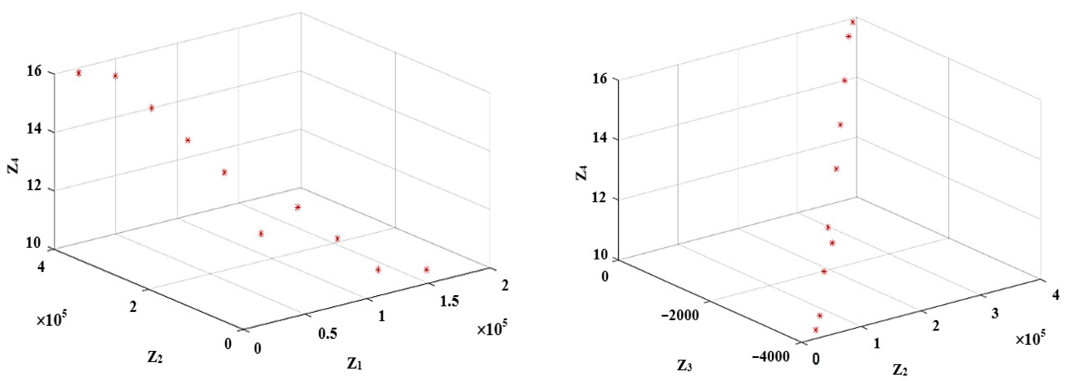
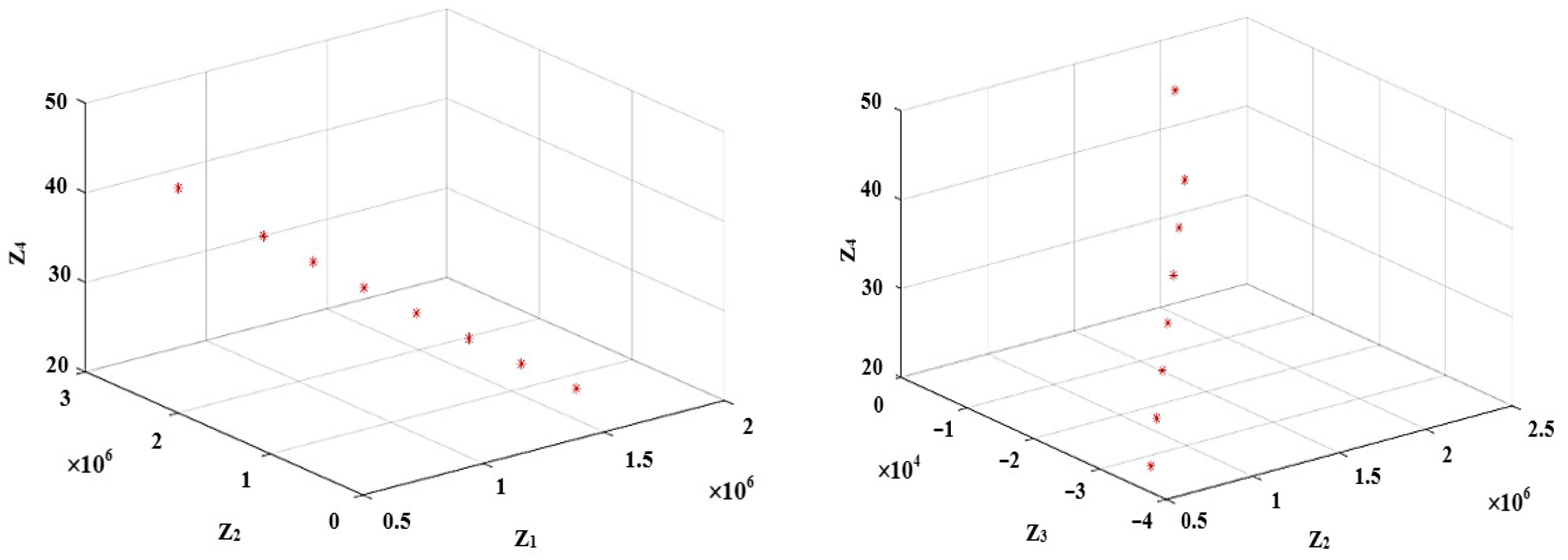
Next, taking into account the values in Table 5 and choosing $r=10$, Equation (59) is employed to derive the values of ${\mathit{\epsilon }}_i$ for each objective function. Doing so and using the $\mathit{\epsilon }$-constraint model in Equation (57), the Pareto solutions are extracted, as shown in

Table 6. The Pareto solutions for the case problems.

	The Small-Size Problem				The Medium-Size Problem				The Large-Size Problem
Objective Function Pareto Solution	Z1	Z2	Z3	Z4	Z1	Z2	Z3	Z4	Z1	Z2	Z3	Z4
1	165,320	43,918	3735	10	493,640	130,690	10,490	11	1,630,951	639,500	34,050	21
2	140,540	81,725	3333	10	418,140	220,750	9377	13	1,474,490	826,440	30,030	24
3	122,160	119,528	2930	11	367,310	310,810	8261	15	1,328,780	1,013,400	26,010	27
4	104,510	157,337	2529	12	281,765	490,919	6029	18	1,183,165	1,200,300	21,980	30
5	89,297	195,136	2125	11	240,850	580,990	4913	20	1,036,904	1,387,300	17,960	33
6	74,089	232,945	1723	13	83,549	941,240	450	27	897,926	1,574,200	13,930	36
7	58,902	270,749	1318	14	-	-	-	-	762,711	1,761,210	9909	39
8	44,060	308,554	917	14	-	-	-	-	506,381	2,013,510	1884	45
9	29,219	346,359	513	15	-	-	-	-	-	-	-	-
10	14,016	384,146	112	16	-	-	-	-	-	-	-	-

. It is notable that in this table, the duplicate values for different values of ${\mathit{\epsilon }}_i$ have been removed. Also, Figure 2, Figure 3 and Figure 4 include triple combinations of the objective functions to make it possible to display them in 3D spaces.

Table 6 and Figure 2, Figure 3 and Figure 4 clearly demonstrate the ability of the $\mathit{\epsilon }$-constraint method to extract various Pareto points and to properly explore the solution space and, therefore, the validity of the method. Another point is the conflict between the objective functions, as indicated by the trend of Pareto solutions in Table 6 and Figure 2, Figure 3 and Figure 4. To this end, the minimization of cost is in contrast with the minimization of the environmental goals. The cost and the social objective functions of the supply chain are also in opposite directions. This means that caring about the social aspects of the supply chain entails paying more, though the effects of these measures on the supply chain profitability may appear in the long term. Also, the Pareto solution that represents the ideal solution for the cost function is alone evident for claiming the supply chain seeking solely the minimization of costs has disappointing performances in the environmental and social dimensions. Thus, a sustainable approach could provide a better alignment of the supply chain with social and national concerns, as observed in other Pareto solutions. The final note in this regard and in line with the model assumptions is that minimizing the costs does not necessarily mean using fewer facilities. That is, sometimes increasing the facilities reduces the transportation and material flow costs on the planned horizon, which in turn can offset the investment costs of the facilities. However, as this cost has to be paid at the beginning of the supply chain, sometimes it is not desirable for the stakeholders or even affordable for them. Overall, the results of this section show that the objective functions are in conflict with each other, and this shows the need to use a multi-objective model for designing a closed-loop supply chain.

4.2. Trend in Aggregate Variables

Another remarkable result of this section is the trends observed in the aggregate variables instead of reporting all variables separately. To do this, variables are categorized into three groups representing, respectively, the total number of established facilities (TF), the total number of processed products (produced, remanufactured, recycled, and disposed) in the planning horizon (TP), and the total transportation in the planning horizon (TV).

Table 7. The aggregate variables of Pareto solutions in the case problems.

	The Small-Size Problem			The Medium-Size Problem			The Large-Size Problem
Aggregate Variable Pareto Solution	TF	TP	TV	TF	TP	TV	TF	TP	TV
1	3	4216	2326	3	19,846	9364	5	69,902	37,772
2	3	3763	2077	3	17,763	8683	5	63,605	36,327
3	3	3310	1851	3	16,074	8603	6	57,225	34,794
4	3	2857	1624	3	12,485	7763	6	50,957	32,438
5	3	2404	1398	3	10,824	6903	7	44,603	29,667
6	3	1951	1171	8	7157	4136	8	38,430	26,879
7	3	1497	945	-	-	-	8	32,211	25,384
8	3	1044	718	-	-	-	11	25,994	23,066
9	3	591	491	-	-	-	-	-	-
10	4	166	210	-	-	-	-	-	-

shows the results of case problems with respect to the mentioned variables.

The results in Table 7 indicate that by reducing the supply chain costs, the level of operation is also reduced. However, sometimes increasing the facilities of the supply chain decreases the supply chain’s overall costs and this will be due to the reduction in other supply chain costs, such as transportation between facilities.

4.3. Sensitivity Analysis

We also carry out a sensitivity analysis on the demand and the number of returned products. For this purpose, three levels are considered; (1) the parameters in the initial values, (2) the parameters multiplied by 1.5, and (3) the parameters multiplied by 2. Figure 5 shows the effects of objective functions versus the changes in the parameters represented by the demand and returned products of the supply chain. The trends of changes indicate the positive and direct effects of demand on all objective functions. However, the effects are more severe on the cost objective function than others. Nevertheless, n an uncertain business environment, the effects of changes in the demand and returned products could be of practical value. That is, if the supply chain and the business context do not have the necessary flexibility to change facilities when these parameters fluctuate, other sustainability goals are diminished inevitably. Therefore, agility and flexibility are strategies that strengthen the supply chain toward sustainability.

5. Discussion

In designing a closed-supply chain, there are various objectives that influence its strategic and operational decisions. Each of these goals addresses a particular aspect of interest to managers, although they can be contradictory to each other. Also, it should balance between long-term and short-term goals because short-term goals target the use of limited resources in order to gain profit in the short term, while long-term goals aim at the possibility of developing the supply chain in the future and flexibility against uncertain events along with equipping the supply chain to earn stable and continuous profits. In this regard, a sustainable perspective provides such a viewpoint to all short- and long-term objectives as well as protecting the rights of future generations with an emphasis on the environment and the development of human societies. In this paper, such a perspective was studied in the design of a closed-loop supply chain, and in this context, new goals were introduced against the conventional goals in supply chain design issues.

As discussed, social and environmental goals, although they have general acceptance, require paying more costs in the supply chain. Nevertheless, paying attention to these dimensions of the supply chain will increase the credibility of the business in the future and somehow guarantee its survival in the future. This is in line with other supply chain design studies that attempt to benefit the sustainable perspective [15,18,20]. Another point is the number of facilities in the supply chain. In a short-term perspective, a smaller number of facilities will cost the investors less and may be favorable for them at the start of their business, but in a long-term perspective, more facilities will reduce costs and release of pollutants in the entire supply chain. Therefore, considering this objective along with other sustainability goals provides a better balance in long-term and short-term decisions and makes sustainability research in the field of the supply chain more aligned with the long-term goals of managers.

The current research could guide managers in policy making and strategic planning in several directions. In line with many scholars, the environmental and social dimensions of the supply chain affect the configuration of the closed-loop supply chain [22]. Improving the distribution planning by including the sustainable goals stemming from the proposed model is also cited as a strategic decision for enhancing the corporate social responsibility of the supply chain [24]. Moreover, the results of the research showed that in strategic thinking, a proper balance between long-term and short-term goals should be created. In this regard, if managers are able to finance more in the initial stages of the business to extend the supply chain facilities, they exhibit high performance in all sustainability goals. Meanwhile, if the supply chain is equipped with appropriate flexibility and agility strategies, it will have a better response to business changes such as demand fluctuations, but otherwise, it will be forced to sacrifice some sustainability indicators for others.

The results of this research clearly showed that the objectives studied in the supply chain design are in contradiction with each other. On the other hand, the $\mathit{\epsilon }$-constraint method extracted Pareto points with high ability, and each point paid more attention to one of the goals. The nature of the contradiction in supply chain design goals was evident even in the sensitivity analysis of the parameters, in that changing the parameters that had a positive effect on one objective function had an adverse effect on some other objective functions. But in any case, one should choose a solution from the Pareto points that reflects the subjective preferences of the decision makers well. In this regard, the fuzzy analytic hierarchy process proposed in [28,29] is beneficial for weighting the objective functions and choosing the most desired solution from the Pareto solution set. The proposed method in this paper only extracted Pareto’s dominant points but did not provide a framework for trade-offs between different solutions that were ultimately preferred by decision makers. Therefore, a supplementary study that can help to choose the final answer correctly and in accordance with the assumptions of the research community is necessary.

6. Conclusions

In this paper, a multi-period, multi-product, and multi-objective function model was presented that aimed to design and optimize a closed-loop supply chain. To do so, two economic objective functions of logistic costs and the number of facilities as well as one environmental and one social objective function were considered. The cost objective functions intended to be minimized included the establishment cost of facilities, the transportation costs between facilities, the processing cost of products, the holding costs of products, and the cost associated with the employee support schemes. In the environmental objective function, the minimization of CO₂ emissions, water usage, and energy consumption was investigated. Moreover, the enhancement of job creation and self-sufficiency throughout the activities of the supply chain were pursued by the social objective function of the paper. Indeed, the main goal of sustainable development is to consider as much as possible objectives that affect human life on a long-term horizon and in coordination with the concerns of future generations. Thus, the proposed paper made contributions to introducing new objective functions in the mentioned dimensions of a sustainable design of the supply chain. To extract the Pareto solutions of the model, the $\mathit{\epsilon }$-constrained method was utilized. The results of the paper in this regard illustrated the conflicts between the objective functions and more emphasis on one of the objective functions in each of the Pareto solutions. We also interpreted the different trends in the solutions, such as the fact that we could not address all design concerns of the supply chain by just emphasizing the total cost of the supply chain. It was shown that this objective function is unable to even address the economic objectives, such as the number of facilities employed in the supply chain. Furthermore, the sensitivity analysis of the demands of the supply chain revealed that these parameters mainly affect the supply chain cost and their effects on the objective functions are slight.

For future research, it is suggested to propose the coordination mechanism within the studied supply chain to provide necessary incentives for cooperation. Also, the use of other multi-objective methods such as compromise and goal programming are suggested. Considering the uncertainty in each of the mentioned parameters of the model could make the model more realistic and increase the capability of the supply chain in response to different changes in the real world and is left as another suggestion for future studies. The closed-loop supply chain is undoubtedly affected by the policies and laws of social and national institutions. Therefore, in line with many emerging investigations, it is worthwhile to study the effect of these measures on supply chain design issues and scrutinize the interventions of the government and other external institutions in future research.

References

Shi, J.; Liu, Z.; Tang, L.; Xiong, J. Multi-objective optimization for a closed-loop network design problem using an improved genetic algorithm. Appl. Math. Model.2017, 45, 14–30. [Google Scholar] [CrossRef]
Govindan, K.; Soleimani, H.; Kannan, D. Reverse logistics and closed-loop supply chain: A comprehensive review to explore the future. Eur. J. Oper. Res.2015, 240, 603–626. [Google Scholar] [CrossRef]
Govindan, K.; Soleimani, H. A review of reverse logistics and closed-loop supply chains: A Journal of Cleaner Production focus. J. Clean. Prod.2017, 142, 371–384. [Google Scholar] [CrossRef]
Zarbakhshnia, N.; Jaghdani, T.J. Sustainable supplier evaluation and selection with a novel two-stage DEA model in the presence of uncontrollable inputs and undesirable outputs: A plastic case study. Int. J. Adv. Manuf. Technol.2018, 97, 2933–2945. [Google Scholar] [CrossRef]
Giri, B.C.; Chakraborty, A.; Maiti, T. Pricing and return product collection decisions in a closed-loop supply chain with dual-channel in both forward and reverse logistics. J. Manuf. Syst.2017, 42, 104–123. [Google Scholar] [CrossRef]
Guarnieri, P.; e Silva, L.C.; Levino, N.A. Analysis of electronic waste reverse logistics decisions using Strategic Options Development Analysis methodology: A Brazilian case. J. Clean. Prod.2016, 133, 1105–1117. [Google Scholar] [CrossRef]
Meade, L.; Sarkis, J. A conceptual model for selecting and evaluating third-party reverse logistics providers. Supply Chain Manag. Int. J.2002, 7, 283–295. [Google Scholar] [CrossRef]
Pourghader Chobar, A.; Adibi, M.A.; Kazemi, A. A novel multi-objective model for hub location problem considering dynamic demand and environmental issues. J. Ind. Eng. Manag. Stud.2021, 8, 1–31. [Google Scholar]
Taleizadeh, A.A.; Haghighi, F.; Niaki, S.T.A. Modeling and solving a sustainable closed loop supply chain problem with pricing decisions and discounts on returned products. J. Clean. Prod.2019, 207, 163–181. [Google Scholar] [CrossRef]
El-Berishy, N.; Rügge, I.; Scholz-Reiter, B. The interrelation between sustainability and green logistics. IFAC Proc. Vol.2014, 46, 527–531. [Google Scholar] [CrossRef]
Van Tilburg, M.; Krikke, H.; Lambrechts, W. Supply Chain Relationships in Circular Business Models: Supplier Tactics at Royal Smit Transformers. Logistics2022, 6, 77. [Google Scholar] [CrossRef]
Guo, S.; Shen, B.; Choi, T.M.; Jung, S. A review on supply chain contracts in reverse logistics: Supply chain structures and channel leaderships. J. Clean. Prod.2017, 144, 387–402. [Google Scholar] [CrossRef]
Mavi, R.K.; Goh, M.; Zarbakhshnia, N. Sustainable third-party reverse logistic provider selection with fuzzy SWARA and fuzzy MOORA in plastic industry. Int. J. Adv. Manuf. Technol.2017, 91, 2401–2418. [Google Scholar] [CrossRef]
Hosseini, S.M.H. A bi-objective model for the assembly flow shop scheduling problem with sequence dependent setup times and considering energy consumption. J. Ind. Eng. Manag. Stud.2019, 6, 44–64. [Google Scholar]
Gholipour, A.; Sadegheih, A.; Mostafaeipour, A.; Fakhrzad, M.B. Designing an optimal multi-objective model for a sustainable closed-loop supply chain: A case study of pomegranate in Iran. Environ. Dev. Sustain.2024, 26, 3993–4027. [Google Scholar] [CrossRef]
Rezaee, A.; Dehghanian, F.; Fahimnia, B.; Beamon, B. Green supply chain network design with stochastic demand and carbon price. Ann. Oper. Res.2017, 250, 463–485. [Google Scholar] [CrossRef]
Zohal, M.; Soleimani, H. Developing an ant colony approach for green closed-loop supply chain network design: A case study in gold industry. J. Clean. Prod.2016, 133, 314–337. [Google Scholar] [CrossRef]
Zarbakhshnia, N.; Soleimani, H.; Goh, M.; Razavi, S.S. A novel multi-objective model for green forward and reverse logistics network design. J. Clean. Prod.2019, 208, 1304–1316. [Google Scholar] [CrossRef]
Tehrani, M.; Gupta, S.M. Designing a sustainable green closed-loop supply chain under uncertainty and various capacity levels. Logistics2021, 5, 20. [Google Scholar] [CrossRef]
Hasan, K.W.; Ali, S.M.; Paul, S.K.; Kabir, G. Multi-objective closed-loop green supply chain model with disruption risk. Appl. Soft Comput.2023, 136, 110074. [Google Scholar] [CrossRef]
Tirkolaee, E.B.; Mardani, A.; Dashtian, Z.; Soltani, M.; Weber, G.W. A novel hybrid method using fuzzy decision making and multi-objective programming for sustainable-reliable supplier selection in two-echelon supply chain design. J. Clean. Prod.2020, 250, 119517. [Google Scholar] [CrossRef]
Sabogal-De La Pava, M.L.; Vidal-Holguín, C.J.; Manotas-Duque, D.F.; Bravo-Bastidas, J.J. Sustainable supply chain design considering indicators of value creation. Comput. Ind. Eng.2021, 157, 107294. [Google Scholar] [CrossRef]
Khorshidvand, B.; Soleimani, H.; Seyyed Esfahani, M.M.; Sibdari, S. Sustainable closed-loop supply chain network: Mathematical modeling and Lagrangian relaxation. J. Ind. Eng. Manag. Stud.2021, 8, 240–260. [Google Scholar]
Jaigirdar, S.M.; Das, S.; Chowdhury, A.R.; Ahmed, S.; Chakrabortty, R.K. Multi-objective multi-echelon distribution planning for perishable goods supply chain: A case study. Int. J. Syst. Sci. Oper. Logist.2023, 10, 2020367. [Google Scholar] [CrossRef]
Amin-Tahmasbi, H.; Sadafi, S.; Ekren, B.Y.; Kumar, V. A multi-objective integrated optimisation model for facility location and order allocation problem in a two-level supply chain network. Ann. Oper. Res.2023, 324, 993–1022. [Google Scholar] [CrossRef]
Ali, S.M.; Fathollahi-Fard, A.M.; Ahnaf, R.; Wong, K.Y. A multi-objective closed-loop supply chain under uncertainty: An efficient Lagrangian relaxation reformulation using a neighborhood-based algorithm. J. Clean. Prod.2023, 423, 138702. [Google Scholar] [CrossRef]
Esmaeilian, S.; Mohamadi, D.; Esmaelian, M.; Ebrahimpour, M. A multi-objective model for sustainable closed-loop supply chain of perishable products under two carbon emission regulations. J. Model. Manag.2023, 18, 285–317. [Google Scholar] [CrossRef]
Wattanasaeng, N.; Ransikarbum, K. Sustainable planning and design for eco-industrial parks using integrated multi-objective optimization and fuzzy analytic hierarchy process. J. Ind. Prod. Eng.2024, 41, 256–275. [Google Scholar] [CrossRef]
Ransikarbum, K.; Pitakaso, R. Multi-objective optimization design of sustainable biofuel network with integrated fuzzy analytic hierarchy process. Expert Syst. Appl.2024, 240, 122586. [Google Scholar] [CrossRef]
Gunantara, N. A review of multi-objective optimization: Methods and its applications. Cogent Eng.2018, 5, 1502242. [Google Scholar] [CrossRef]
Lahri, V.; Shaw, K.; Ishizaka, A. Sustainable supply chain network design problem: Using the integrated BWM, TOPSIS, possibilistic programming, and ε-constrained methods. Expert Syst. Appl.2021, 168, 114373. [Google Scholar] [CrossRef]
Figure 1.
The forward and reverse flows in the closed-loop supply chain.
Figure 2.
The Pareto solutions for the small-size problem in 3D space.
Figure 3.
The Pareto solutions for the medium-size problem in 3D space.
Figure 4.
The Pareto solutions for the large-size problem in 3D space.
Figure 5.
The effects of demand changes on the objective functions, where sub-figures (a–d) show those effects on the objective functions Z1, Z2, Z3, and Z4, respectively.