1. Introduction
Freight forwarding is considered an essential service today, and with the expansion of the e-commerce market, the global freight forwarding industry is undergoing steady growth. However, there are two major challenges faced by freight forwarding services on a global scale. The first challenge is the need to reduce CO
2 emissions, which account for about 76% of greenhouse gas emissions [
1], as freight transportation is responsible for approximately 7–8% of carbon emissions and is a significant contributor to global warming. Unlike many other industries that have successfully reduced their emissions over the years, the freight transport sector continues to increase its emissions and is recognized as one of the most difficult sectors to decarbonize [
2].
The second challenge is the shortage of truck drivers, which is exacerbated by the growing demand for freight transportation services. It is estimated that there will be a global shortage of more than 7.0 million truck drivers by 2028 [
3]. Factors contributing to this shortage include low wages and an aging population with low birth rates. It has long been recognized that wages in the transportation industry are relatively low compared to other industries. This is due to not only poor management within transportation companies but also the expansion of the e-commerce market, which has led to an increase in high-mix, low-volume transportation. As a result, transportation efficiency has been compromised, and the industry has been operating on tight margins. In addition, shippers continue to rationalize logistics costs, putting further pressure on cost compression. These factors have made it difficult to improve freight revenues, and the power dynamics between companies have normalized unfavorable conditions for transportation companies. Under these circumstances, the entire transportation industry could be at risk if the truck driver shortage worsens.
To address these challenges, the concept of the Physical Internet (PI) has gained significant attention as an effective way to improve logistics efficiency [
4]. The PI is seen as a way to take logistics into the next generation of transformation. The realization of the PI would contribute to the establishment of a sustainable society by reducing the number of trucks required for transportation, minimizing fuel consumption, and reducing greenhouse gas emissions. To achieve this, it is crucial to establish a network in which logistics resources such as warehouses and trucks are shared among multiple companies. However, if the locations of shared warehouses and the routes of trucks between regions are not optimized, it can lead to transportation delays and problems such as overstocking or understocking. These challenges hinder the realization of the PI and compound problems such as rising logistics costs and shortage of available truck drivers. Therefore, it is necessary to propose a new algorithm that optimizes the location of shared warehouses and truck routes between regions while taking into account the PI concept.
The primary objective of this study is to provide recommendations and guidelines for transforming the concept of the PI into a practical reality. A number of factors have been taken into consideration, including the distribution of existing logistics facilities, customer locations, and the capacity of these distribution centers. Based on these considerations, we propose innovative solutions to determine the optimal locations for logistics facilities and optimize truck routes, ultimately improving overall efficiency and reducing carbon emissions.
Compared to existing studies, our contributions are fourfold. First, this study applies the concept of the PI to the study of logistics networks. It addresses fundamental solutions to common global challenges in freight transportation services, such as reducing greenhouse gas emissions, alleviating the shortage of truck drivers, and improving profit margins in the transportation industry. Second, we extend the hybrid genetic algorithm (GA) and Lin–Kernighan heuristic (LKH) method proposed by Pan et al. [
5]. In this study, we propose a new model that incorporates the bias of demographic information in each region into the GA to further improve the model performance, which is the novelty of our research. In addition, we simulate the use of existing logistics centers as warehouses in conjunction with the concept of the PI, which allows optimization without incurring additional investment. Third, we simulate the model using real data. The hybrid method, which combines the optimal number of clusters, GA, and LKH-3, is applied to geographic information system (GIS) data, including factory locations, logistics hubs, and critical logistics roads. The model can be further applied with real data sets in other regions or countries to solve practical social problems. Fourth, in addition to optimizing transportation routes based on LKH, we use the Routes API of the Google Maps platform to calculate routes that incorporate actual traffic factors such as road type (expressways and general roads), vehicle type (gasoline, EV, hybrid, etc.), and traffic conditions in each section. The Routes API provides a more realistic approach than other delivery route optimization models because it takes into account various factors that influence route selection.
The remainder of this paper is organized as follows.
Section 2 reviews the research progress in the area of the PI and route optimization.
Section 3 provides a step-by-step description of our proposed model.
Section 4 briefly describes the data used in this study.
Section 5 presents the experiments, demonstrating the effectiveness of our approach through empirical results, and finally,
Section 6 summarizes our conclusions.
2. Previous Works
2.1. Physical Internet Related Research
The concept of the PI was introduced in 2010 by Montreuil et al. [
4]. Their definition of the PI describes an open and global logistics network based on the efficient and sustainable interconnection of all aspects of the logistics process. In principle, this means transforming traditionally closed and operational logistics networks to function more like the communication mechanisms of the internet.
The vision of the PI is to create a sustainable global system for transportation, handling, storage, delivery, and utilization. To achieve this ambitious goal, Montreuil et al. [
4] proposed the use of smart technologies, modular resources such as PI containers and PI movers, and infrastructure such as PI nodes and PI hubs. Treiblmaier, Mirkovski, and Lowry [
6], Pan et al. [
7], and Münch et al. [
8] have provided comprehensive research reviews on the PI.
Despite its potential, the PI is a relatively new concept that needs to be evaluated in terms of its adaptability to real logistics systems, transportation infrastructures, sustainability, and societal benefits.
Many other papers deal with vertical cooperation in the PI, focusing on cooperation between different modes of transport.
2.1.1. Vertical Collaboration
Vertical collaboration is when two or more parties, such as shippers and logistics providers, share resources, responsibilities, and information for efficiencies [
9]. Vertical collaboration is one of the most important themes in PI-related research. Ji et al. [
10] developed an integrated model that incorporates production, inventory, and logistics aspects within the PI framework. They introduced a mixed-integer linear programming formulation to evaluate the cost performance of the PI compared to conventional logistics systems. Experimental results confirm the superior cost performance of the PI, coupled with comparable or improved service levels. In particular, cost savings are primarily associated with reduced fixed vehicle costs and variable transportation costs. These savings become more significant as the network expands, with reductions in fixed vehicle costs playing an increasingly important role.
Kulkarni et al. [
11] designed a hyperconnected logistics hub network that is resilient to disruption risks. They proposed two solution approaches based on the PI framework and integer programs. The designed network showed a significant increase in its ability to withstand disruptions compared to traditional logistics networks, highlighting the value of hyperconnectivity in designing efficient and resilient logistics networks.
Achamrah et al. [
12] proposed a dynamic and reactive routing protocol for PI subnetworks. The purpose is to enable dynamic, self-initiated, multi-hop routing between nodes and to ensure continuous connectivity in the face of network disruptions.
Hettle et al. [
13] proposed a mixed-integer programming-based method for clustering urban logistics in hyperconnected networks. The method aims to generate robust, geographically compact, and demand-balanced clusters while minimizing expected operating costs.
Mohammed et al. [
14] designed a multilayer supply chain network with an emphasis on sustainability and resilience. They developed a fuzzy four-objective optimization model that considers the resilience performance of facilities and the uncertainty of input parameters, in addition to traditional economic objectives. They proposed a method to minimize the environmental impact and maximize the resilience performance of the supply chain network.
Many other papers have addressed vertical cooperation in the PI, focusing on cooperation between different modes of transport [
15,
16].
2.1.2. Horizontal Collaboration
Horizontal collaboration between logistics service providers is another important theme in PI-related research. Horizontal collaboration is a partnership between entities that supply similar services or products in order to achieve economies of scale by cooperating. Often, these companies are competing directly with each other [
17]. Fazili et al. [
18] quantified the advantages and disadvantages of the PI in terms of optimizing truck routing, considering constraints related to the maximum return time of truck drivers. Their results show that the PI allows higher efficiency in terms of truck travel distance and time, lower greenhouse gas emissions, and lower social costs. It also allows more truck drivers to return home at the end of their shifts, regardless of traffic conditions.
Many researchers have developed models that incorporate various constraints to test the feasibility of logistics networks in the PI and to further investigate the optimality of inventory management decisions and sourcing methods within these networks [
19]. Sarraj et al. [
20] developed a model for asynchronous shipping and container creation within an interconnected service network. This model optimized container routing and simulated the minimization of transportation asset utilization. The results showed a roughly 17% increase in transport fill rates and a potential 60% reduction in carbon dioxide emissions, without compromising lead times or operating costs.
Chargui et al. [
21] proposed a multi-agent model for persistent truck scheduling and container grouping at PI hubs. The model aimed to minimize the number of trucks used, the total distance traveled by PI containers, and the total truck delay time. However, it primarily addressed internal disruptions and overlooked other external disruptions (e.g., train delays and unexpected truck arrivals) and the need for temporary storage zones.
In the context of uncertain demand and stochastic supply disruptions, Yang et al. [
22] investigated the single-product inventory problem within PI. Their experiments revealed that the inventory model of the PI outperforms conventional models, especially under conditions of demand variability and supply chain disruptions.
Pan et al. [
5] studied a collaborative delivery network using parcel lockers using a GA and LKH to optimize parcel flow paths and vehicle flow. Their results suggest that this model can be flexibly extended to analyze larger delivery systems while maintaining computational feasibility.
This research focuses on the horizontal collaboration for the truck delivery. From this literature review, it is noticeable that research on the PI has expanded significantly over the past decade, with various models proposed to validate the practicality of logistics networks within the PI framework. However, to the best of our knowledge, a comprehensive model that integrates the PI concept with optimal logistics hub placement, route optimization, and demographic data has not been reported. Therefore, motivated by the lack of research, this work aims to fill the research gap by proposing a novel model by introducing a weighted demography model that addresses the optimal placement of logistics hubs and the optimization of delivery routes in the context of the PI with empirical validation using real-world data.
2.2. Location Routing Problem
The location routing problem (LRP), which combines the facility location problem (FLP) and the vehicle routing problem (VRP), has been an important research topic especially in the last two decades. A trend shows that the emphasis of LRP research has been shifting from deterministic to stochastic data [
23].
Sluijk et al. [
24] reviewed research on the two-echelon VRP applied in distribution systems including express delivery, grocery, and hypermarket product distribution, multimodal freight transportation, urban logistics, and e-commerce and home delivery services. The authors found that the genetic algorithm is one of the most important methods for population-based heuristics.
Schneider and Drexl [
25] reviewed the literature on the LRP. In their review, the GA is mentioned as one of the effective metaheuristics for solving the LRP.
Taking into account the existing literature, we decided to adopt the GA with stochastic data as the foundation of the model examination and propose a hybrid model combining LKH-3 with weighted freight flow.
3. Proposed Methodology
In this section, we first explain the differences between traditional logistics and next-generation logistics systems transformed by the PI. Then, we describe the steps that led to the final presentation of the proposed model.
3.1. Traditional Logistics Systems and Next-Generation Logistics Systems Transformed by the PI
In the traditional logistics framework, each logistics provider operates independently across the entire supply chain process. This includes receiving goods from suppliers, temporarily storing them in warehouses, transporting them, and finally delivering them to customers. This fragmented approach results in a separation of transportation and warehouse management, leading to inefficiencies.
In contrast, the next-generation logistics systems transformed by the PI enable collaboration among logistics providers, with warehouses serving as central hubs. This collaborative approach enables the creation of a shared distribution network that offers numerous benefits. These benefits include increased efficiency in truck loading, improved warehouse utilization, reduced financial costs, shorter vehicle miles traveled, and a reduced environmental impact associated with distribution activities.
To fully realize these benefits when implementing a collaborative distribution network, it is critical to determine the optimal location and number of logistics hubs. In addition, it is important to leverage existing supplier logistics facilities and distribution warehouses to avoid new investments and site unavailability.
3.2. Assumptions
To construct a model of a joint delivery network, let
be the set of suppliers and
the set of customers. The delivery task denoted by
transfers goods with
from supplier
to collection point
, between logistics nodes
in set
and collection point
, from where they are delivered to customer
. The set
is assumed to correspond to the main logistics routes as defined by the Ministry of Land, Infrastructure, Transport, and Tourism (MLIT) in Tokyo, Japan. In the context of our modelling, we assume that each customer (called distributor) generates a single delivery request destined for a single customer (distributor). Given this underlying assumption, the set of demands
(
) originating from supplier
(for customer
) contains exactly one delivery task. Furthermore, in order to keep the model simple, we do not specify collection or delivery times.
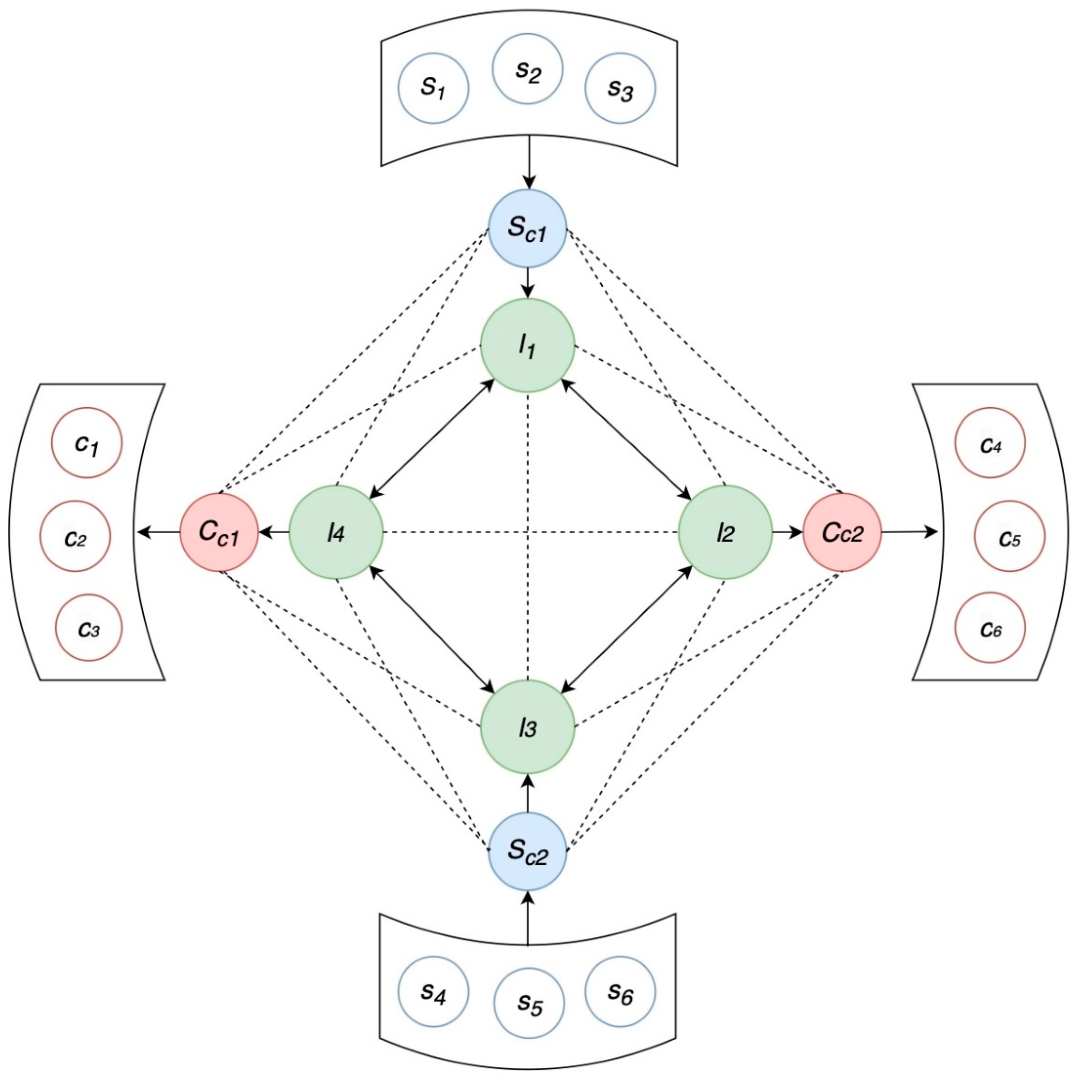
Figure 1 illustrates the delivery flow diagram in the context of the PI. Dotted lines indicate potential flow routes, while solid black arrows indicate the chosen routes. Suppliers (
) and customers (
) are grouped into clusters, and their respective goods are transported through collection points
,
and distribution points
(
Figure 1).
3.3. Logistics Nodes
The logistics nodes set, denoted as , includes all logistics nodes identified by their geographical positions. Within , there exists a delivery task represented as . Each logistics hub is equipped with a capacity of . We assume the existence of a transport service for the exchange of goods between logistics nodes, if necessary.
The costs of setting up logistics hubs are not taken into account, and their capacities are known a priori. Accordingly, the collection points , are connected to the nearest logistics hub. It is assumed that , can replace the logistics hub l that is supposed to be newly generated.
3.4. Transport by Trucks
For the transport of goods, a set of trucks can be operated, and these vehicles are associated with a collection point or a distribution center. The set of vehicles includes three types of trucks with different carrying capacities . Operational costs, consisting of financial and environmental costs due to truck ownership, are not considered.
3.5. X-Means Method
The X-means approach, originally introduced by Pelleg and Moore [
26] as a variant of hierarchical clustering based on ratios, extends the capabilities of the K-means method. Unlike K-means, which requires a predetermined number of clusters, X-means autonomously determines an optimal number of clusters for the given data. In this research, we employ an extended version of the X-means algorithm as refined by Ishioka [
27]. This refinement incorporates considerations of variance disparities between successively partitioned sub-clusters and uses an approximate log-likelihood calculation method to improve computational efficiency.
3.6. Constraints
The developed model has a three-stage structure. First, an arbitrary number of given suppliers and customers are clustered to obtain the supplier agglomeration and the customer agglomeration . Next, we consider the least-cost trucking network flow problem related to the generation of an appropriate number of distribution points between the agglomerations, and finally, we address the multi-depot capacity vehicle routing problem between the agglomerations and the distribution points. We employ the fuzzy c-means method to group the provided suppliers and customers into clusters, with no predefined limit on the number of clusters. In this particular context, we address the scenario where each supplier and customer can have partial membership across multiple depots. Consequently, we have chosen the fuzzy c-means method, as it effectively captures the extent of membership of each data point within a cluster, making it the optimal clustering approach for our problem.
Clustering via the fuzzy c-means approach was executed through the following steps:
Initialize the attribution degree () randomly.
Compute the cluster centers for each cluster using the current attribution degree ().
Update the attribution degree () of element to cluster i using the center calculated in (2).
Continue to iterate through the assignment and adjustment steps until the membership degrees undergo minimal change.
where
is the fuzzification degree.
For the formulation of the multi-depot capacity vehicle routing problem, we focus on the former because the formulation for moving goods from the supplier’s collection point to a logistics node is very similar to that of moving goods from a customer’s collection point to a logistics node. Given a set of vehicles tasked with collecting goods at a collection point , let if a vehicle moves from node to node (either a supplier or a collection point) () and if it does not move. The variable is used to denote the transport route of trucks from the supplier’s depot to the logistics depot , and the variable is used to denote the transport route of trucks from the logistics depot to the customer depot . Demand, vehicle, and distribution center capacity constraints are not directly considered in the multi-depot capacity vehicle routing problem between distribution centers. Instead, they are considered in the least-cost truck transport network flow problem.
In the formulation of the least-cost trucking network flow problem, we classify collection points, logistics nodes, and trucks as intermediate nodes, whereas suppliers and customers are designated as ‘origin’ and ‘destination’ nodes, respectively. The objective is to efficiently distribute goods across the network while adjusting the capacity constraints at each node. This optimization aims to meet the demand requirements at the origin and destination nodes while minimizing the total truck mileage. The binary variable
represents the flow variable, specifying whether the goods in the delivery task
pass through node
and node
, and adapts all capacity constraints through
. Next, we consider the minimum-cost trucking network flow problem together with the multi-depot capacity vehicle routing problem. If node
is a supplier, the binary variable
is defined by the vehicle flow variable
. The right-hand side of (4) represents the loads sent by the supplier. The vehicle
is determined by the supplier
, logistics base
. The maximum value of the right-hand side is
.
Once the connection between the parcel flow and vehicle flow variables is set up, the capacity constraints for vehicles and depots are imposed using the variable
.
The left-hand sides of (5) and (6) determine the total quantity of goods carried to truck and distribution point , respectively. The same capacity constraints as in (5) can be applied to the trucks used.
3.7. Objective Function
Our goal is to optimize both the total cost of truck use and the number of logistics hubs. In other words, we want to minimize total truck distance travelled while minimizing the number of logistics hubs. However, given the conflicting nature of these two factors, our ultimate focus is to achieve an ideal balance between minimizing truck distance and reducing the number of logistics hubs. The objective function is given as follows.
Equation (7) represents the distance between logistics hubs, while Equations (8) and (9) represent the distances between logistics hubs and supplier catchments and between logistics hubs and customer catchments, respectively. Equation (10) determines the number of logistics hubs used () and limits the number of logistics hubs used by a maximum value . Equation (11) represents the difference between the total cargo of the logistics depots and the capacity of the logistics depots. Equation (12) represents the difference between the sum of truck loads and the capacity of the logistics base.
3.8. LKH
The LKH-3 heuristic solver, an improved version of the LKH-2 xv (Lin–Kernighan–Helsgaun travelling salesman problem solver) algorithm developed by Helsgaun [
28], provides a broader problem-solving capability. While LKH-2 was primarily designed to solve travelling salesman problems (TSPs), LKH-3 demonstrates its adaptability in solving a wide range of problems, including those with capacity, time, pickup, and distance constraints (known as vehicle routing problems or VRPs). It also excels at handling facility processing constraints and multi-travelling salesman problems (mTSPs), while allowing sensitivity analysis to guide and constrain the solution search.
It is available free of charge for academic and non-commercial use, and users can freely obtain the source code for implementation. In the context of our research, we have used the Python library known as elkai [
29], which is based on LKH-3. This library has been shown to provide optimal solutions for problem sizes up to N = 315, surpassing the accuracy of Google’s OR tool. It also simplifies the retrieval of results with a single line of code.
3.9. Combining Genetic Algorithms with LKH-3 in a Hybrid Approach
Solving routing problems with numerous variables derived from the TSP is a challenging and time-consuming task using mathematical methods and search algorithms. Since our problem surpasses previous ones in terms of generality and complexity, we have adopted a hybrid approach that combines a GA and LKH-3 based on the two-layer structure of our proposed model. Our algorithm is inspired by Pan et al. [
5], and we add our novelty by introducing a new bias
φ.
The GA focuses on locating the optimal logistics hubs, and once these locations are determined, the LKH takes over the evaluation of solutions and the optimization of truck transport routes. In order to respect the capacity constraints of trucks and hubs, we introduce penalty conditions into the adaptive computations of the GA.
The bias
φ is the amount of freight flow in each prefecture divided proportionally by the population of each municipality. This bias increases the probability that logistics hubs will be located in places with high freight flow (population). This allows us to extend the algorithm proposed by Pan et al. [
5] to intercity logistics.
Equation (13) is an equation for calculating the expected total mileage of a truck. Equation (13) is the sum of (7), (8), and (9). Equation (14) is the penalty for exceeding the capacity of logistics hubs (nodes) and trucks, which is added to the GA’s adaptability whenever capacity constraints are violated in order to account for capacity constraints in LKH-3. Equation (14) is the sum of (11) and (12). Equation (10) determines the number of logistics hubs to be used () and limits the number of logistics hubs to be used by a maximum value n. In other words, on the right side of Equation (11) defines the total capacity of logistics hubs and penalizes the difference from the total capacity.
3.10. Final Presentation of the Proposed Model
In the GA, the initial population size is predetermined and is denoted as (
). This population size remains constant at the end of each iteration (generation), although it may change during the evolution of each generation. Initially, after obtaining instance and parameter information,
candidate solutions are randomly generated, and the fitness of each solution is evaluated.
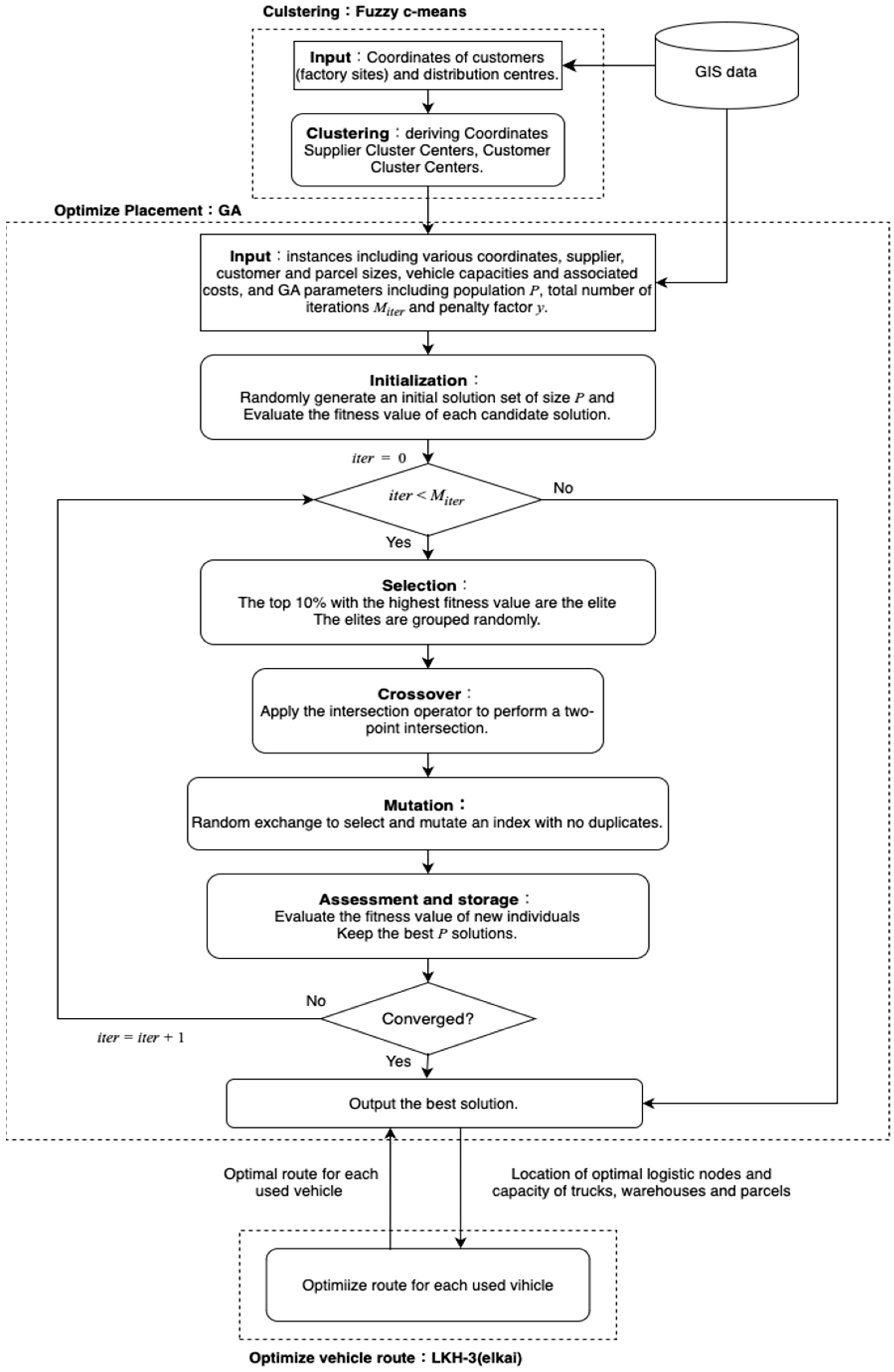
Figure 2 outlines the overall model’s output procedure.
Use the elbow method and shape analysis to determine the optimal number of clusters.
Employ the fuzzy c-means method for clustering and calculate the coordinates of both supplier cluster centers and customer cluster centers.
Determine the coordinates and number of logistics nodes with the GA based on the coordinates of supplier cluster centers, customer cluster centers, distribution centers, factory locations, and warehouse capacity.
Generate appropriate routes using elkai based on the coordinates of logistics nodes determined by the GA and considering truck and container sizes.
Evaluate the degree of fitness and save the best GA corresponding to the highest degree of fitness.
Iterate steps 3 to 5 a total of n times.
Display the coordinates of the best logistics nodes and truck transport routes.
The pseudocode for the proposed model is presented in
Appendix A (Algorithm A1).
4. Data Description
In this section, we describe the data sets used in this research, including GIS data, Open Street Map data, warehouse and truck information, and Routes API. Since GIS data play a critical role in ensuring the accuracy and reliability of our research findings, we carefully selected appropriate GIS data to produce accurate results in line with our research objectives.
4.1. Location Data for Distribution Centers
We obtained geographic data for logistics facilities from the National Land Information Download Site [
30]. For our research, we used GIS data as of July 2013 provided by MLIT on an open-source basis. The logistics facilities covered include container terminals, air freight terminals, rail freight stations, bonded areas, truck terminals, and wholesale markets. The data are stored in shapefile format. As part of our preliminary data preparation, we merged and transformed the prefectural data for the Kansai (western Japan) region, which includes the Osaka, Kyoto, Shiga, Nara, Hyogo, and Wakayama prefectures, into a format suitable for our research purposes.
4.2. Location Data for the Factory Sites
The factory locations were obtained from the MLIT website [
31], which provides national land data for download. For this research, we used GIS data dated 27 March 2009 in shapefile format. In the pre-processing phase, we extracted the vertex coordinates of the polygons of each factory site and used their centroids as the coordinates of the industrial sites. In addition, we collected prefectural data for the Kansai region and transformed them into a format suitable for our study.
4.3. Data on the Area of Distribution Centers (Warehouses)
In this study, the average total floor area data from 2019 to 2022 from the “Statistical Survey of Construction Starts” obtained from e-Stat, a government statistics portal site [
32], were used as an indicator of the total floor area of logistics centers. In addition, to determine the capacity of individual warehouses and distribution centers, the floor area of each building was calculated by dividing the cumulative floor area of warehouses from 2019 to 2022 by the total number of buildings. In addition, the allowable storage capacity (in cubic meters) was calculated assuming a storage height of 5.5 m and an occupancy rate of 40%. The resulting average allowable capacity over the four-year period was adopted as the capacity of the warehouse and distribution center used in the simulation, as shown in
Table 1.
4.4. Truck Data
Data on truck cargo dimensions were obtained from Isuzu Motors Limited (Tokyo, Japan) [
33], a Japanese automobile manufacturer that primarily produces trucks, buses, and other commercial vehicles. We obtained PDF files of product catalogs from Isuzu Motors, from which we extracted vehicle dimensions. In addition, data from ELF for light-duty trucks (2 tons), FORWARD for medium-duty trucks (4 tons), and GIGA G-CARGO for heavy-duty trucks (10 tons) were included in the analysis. The hauling capacity of the trucks was calculated as the volume of the cargo compartment, and this volume was adopted as the hauling capacity parameter of the trucks used in the simulation (referred to as “capacity” in
Table 2).
4.5. Routes API
The Routes API is a new addition to the Google Maps (Google) platform that is designed to enhance the functionality and efficiency of both the Directions API (used for one-to-one route searches, distance calculations, and travel time estimates between origin and destination) and the Distance Matrix API (used for route searches, distance calculations, and time estimates for multiple destinations). By using the Routes API, it is possible to access search results that were previously inaccessible using the traditional Directions and Distance Matrix APIs while significantly increasing the speed at which these results are obtained. In this research, we used the API’s capabilities to determine the most efficient truck routes using data on distribution center locations obtained via the GA in conjunction with real-world road data.
5. Presentation of the Results and Evaluation of the Proposed Model
5.1. Parameters for the GA
The GA settings are presented in
Table 3, and these values can be changed on a trial-by-trial basis.
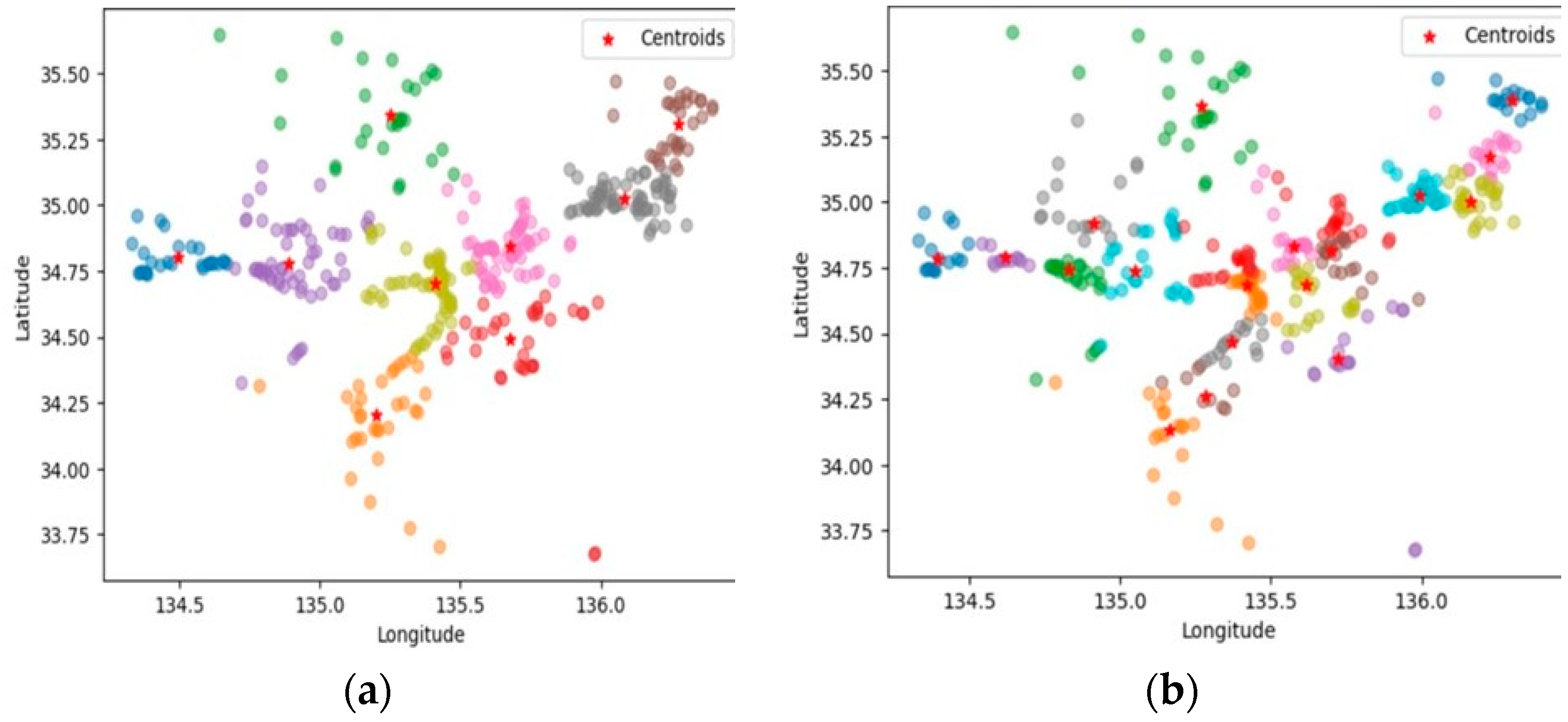
5.2. Clustering Based on the Fuzzy c-Means Method
As shown in
Figure 3a,b, distribution centers and factory sites were clustered using the fuzzy c-means method. The number of clusters in each group was determined using the X-means method. The difference between the fuzzy c-means method and conventional methods such as the k-means method is its inherent flexibility, which allows data points to be assigned to multiple clusters with adaptability. In conclusion, the fuzzy c-means method was selected as the most appropriate choice for clustering distribution centers and similar entities due to its versatility.
5.3. Depiction on Map (without Bias)
The map shows the actual simulation results for determining the optimal placement of logistics centers and the corresponding delivery routes. The optimal routes are represented by black lines, suppliers by red dots, supplier cluster centers by red pins, customers by blue dots, customer cluster centers by blue pins, and logistics hubs by green pins. To compare the changes with and without bias
φ,
Figure 4 shows the GA without bias in terms of adaptation. The adaptivity formula is as in (16).
5.4. Depiction on Map (with Bias)
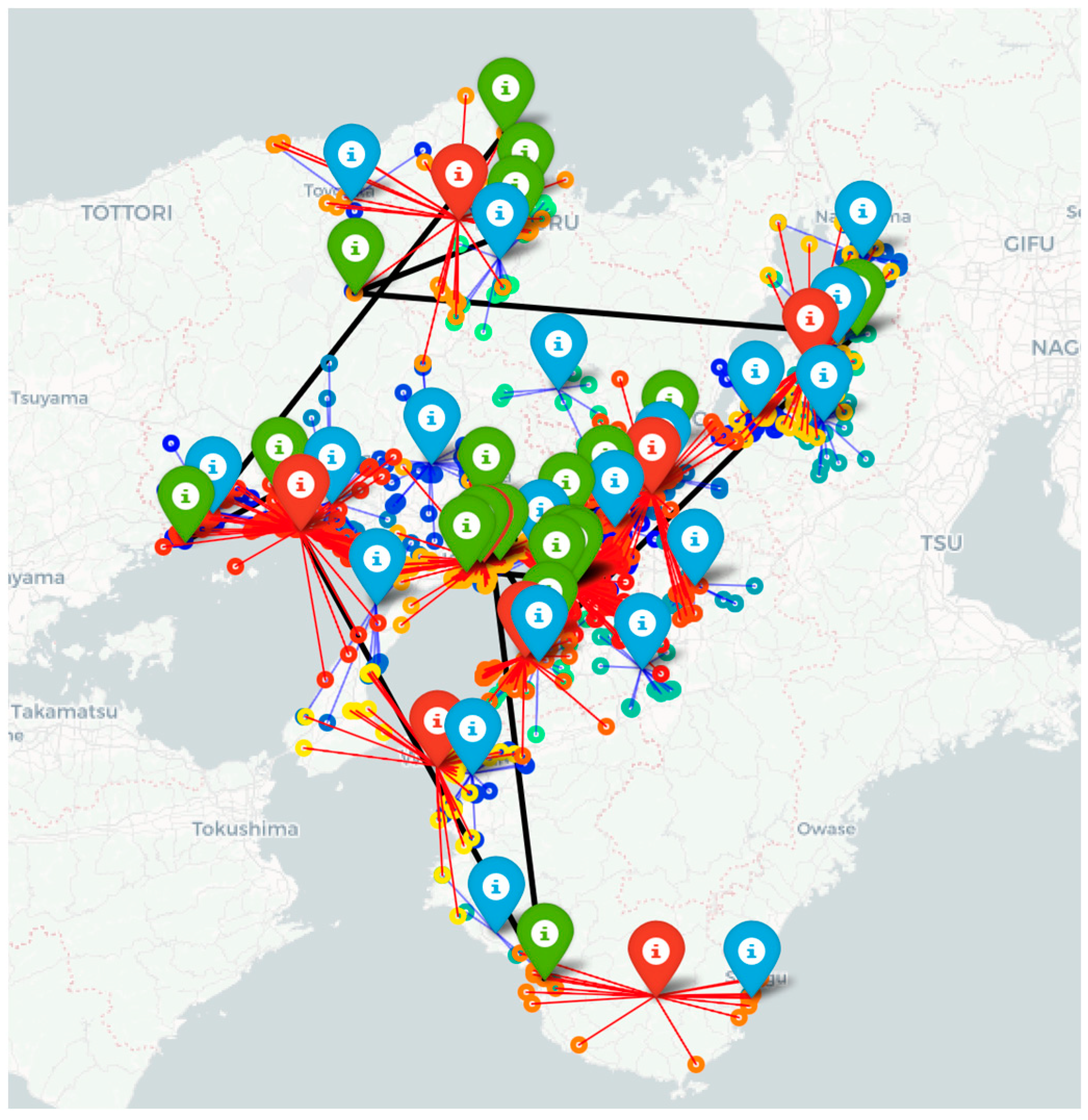
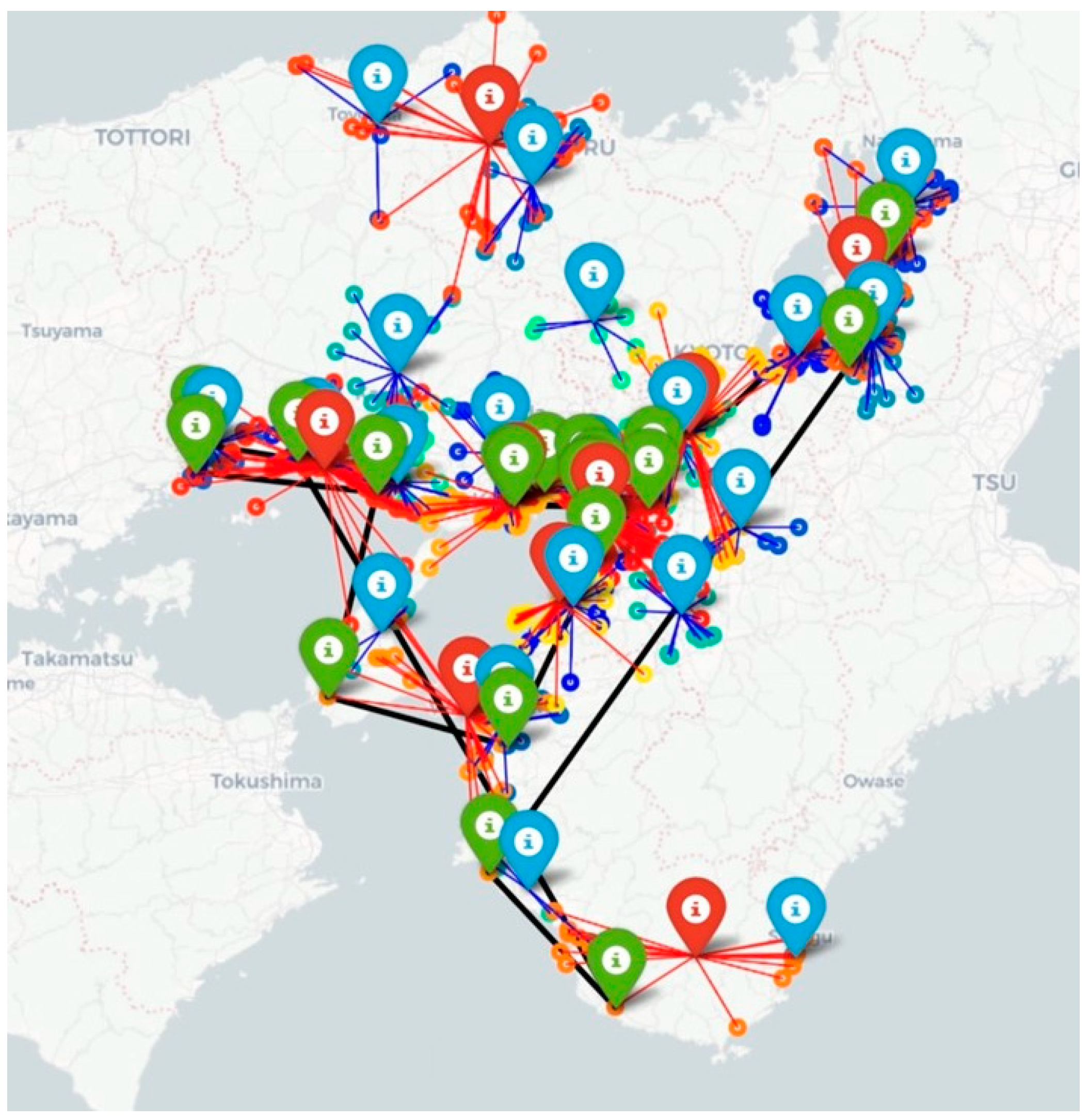
As shown in
Figure 5, the map shows the actual simulation results for determining the optimal placement of logistics centers and the corresponding delivery routes. Optimal routes are represented by black lines, suppliers by red dots, supplier cluster centers by red pins, customers by blue dots, customer cluster centers by blue pins, and logistics nodes by green pins. In contrast to
Figure 5, a bias is added to the adaptivity of the GA, as in Equation (15). As can be seen from the results, logistics hubs tend to be located in coastal areas with high population and flow volumes.
5.5. Evaluation of the GA’s Performance
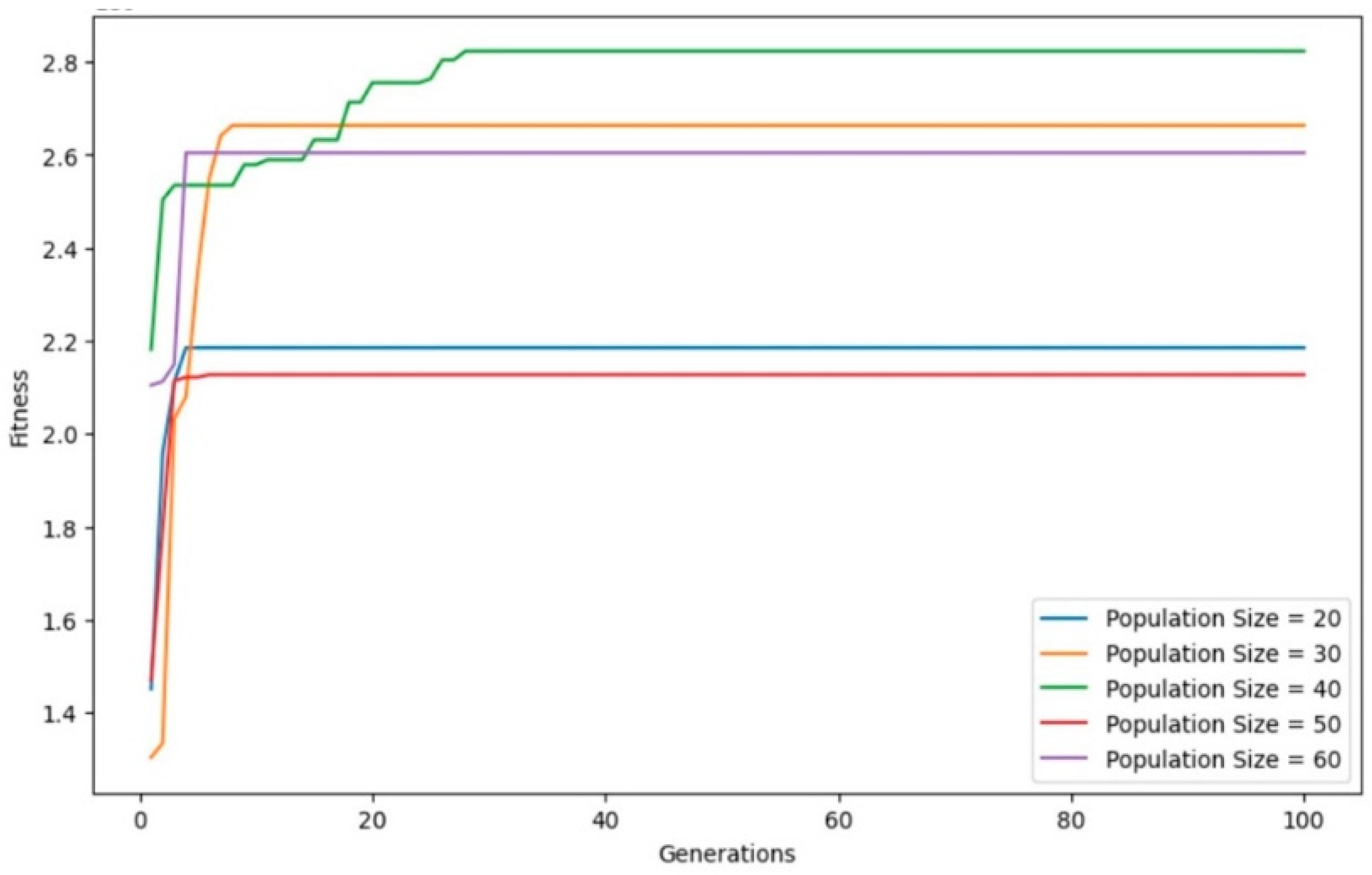
The graph in
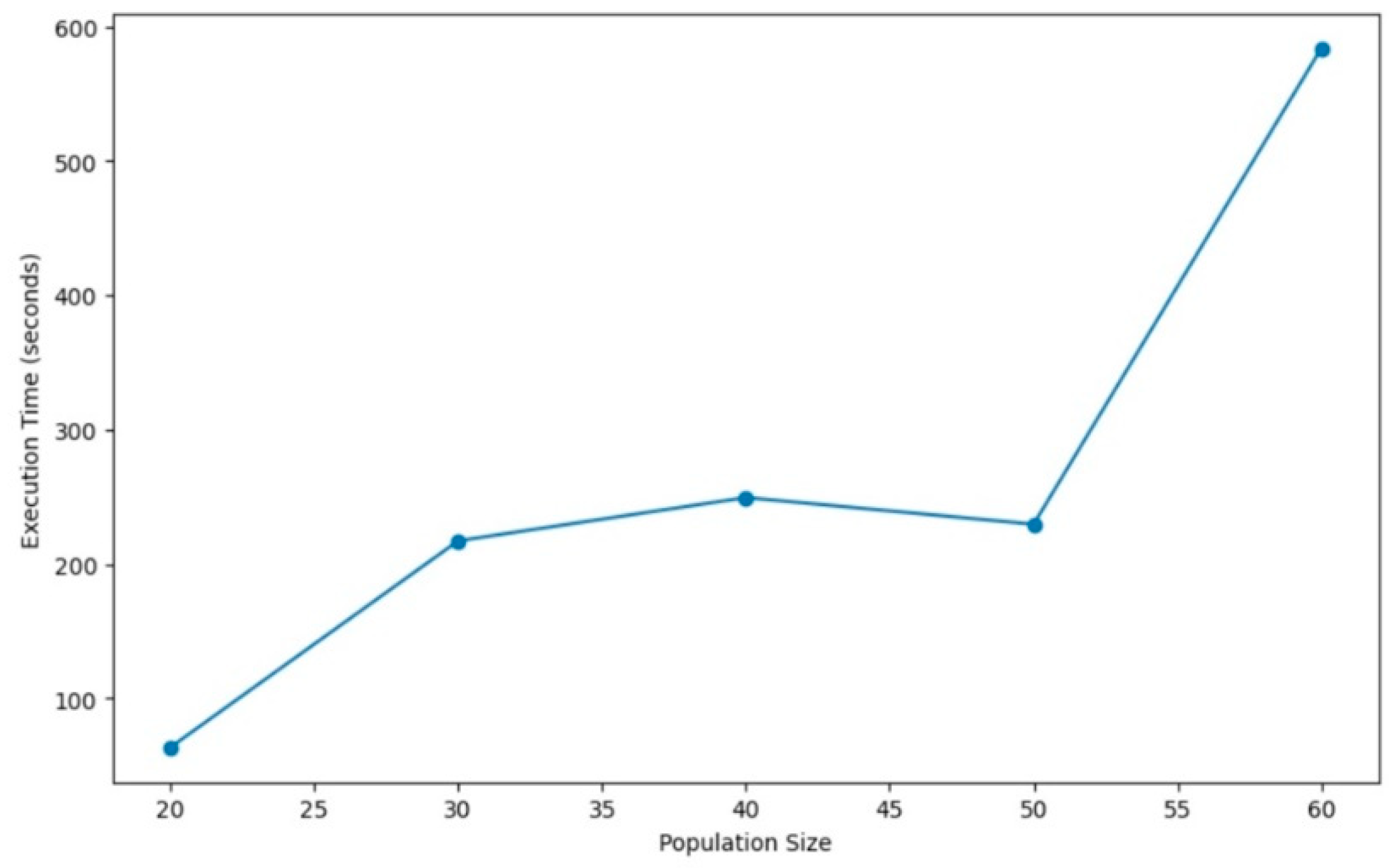
Figure 6 shows the evolution of the level of adaptation of the GA for different numbers of populations (20, 30, 40, 50, and 60). In the first generations, the population had a low level of fitness. Once the GA was initiated, the level of adaptation increased rapidly in the early stages of evolution. Later, after a certain number of generations, the level of adaptability reached a stable state and became less variable. The graph in
Figure 7 shows the evolution of the processing speed with different numbers of populations (20, 30, 40, 50, and 60). The larger the number of populations is, the relatively slower the convergence.
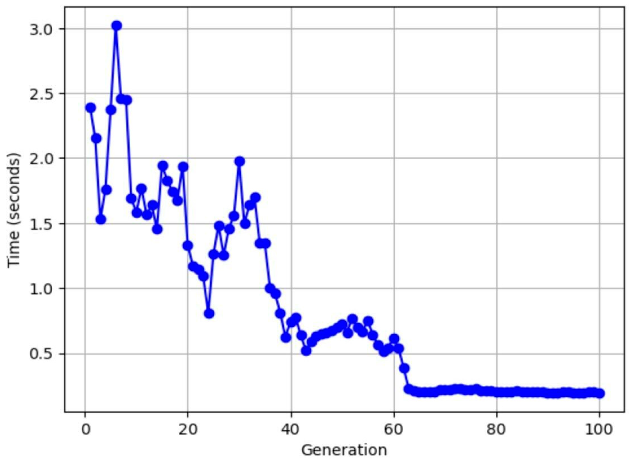
Figure 8 shows the evolution of the processing speed in the number of generations with a population number of 40. The speed decreases as the number of generations increases. The cumulative time is about 200 s (consistent with the results for the degree of adaptation).
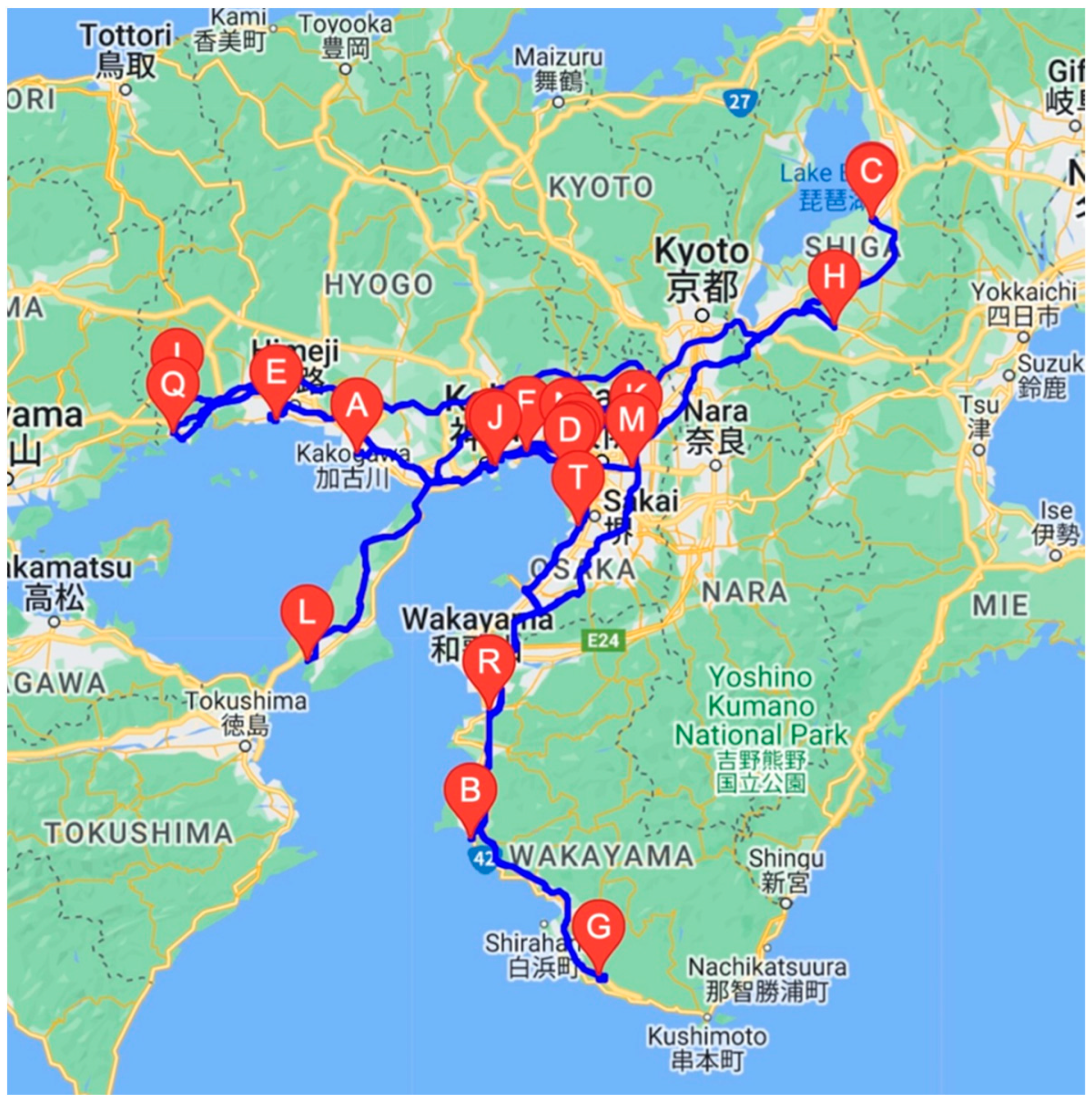
5.6. Depiction of Transport Routes along Real Roads
The hybrid approach combining LKH-3 (elkai) and the GA, as shown in
Figure 9, is used to establish transport routes connecting logistics hubs by minimizing straight-line distances. These routes do not take into account the actual road network. To obtain transport routes along real roads, we used the coordinates of logistics bases determined by the GA and the Routes API from the Google Maps platform. The results are shown in
Figure 9, where the blue lines represent the optimal routes and the pins represent the logistics hubs.
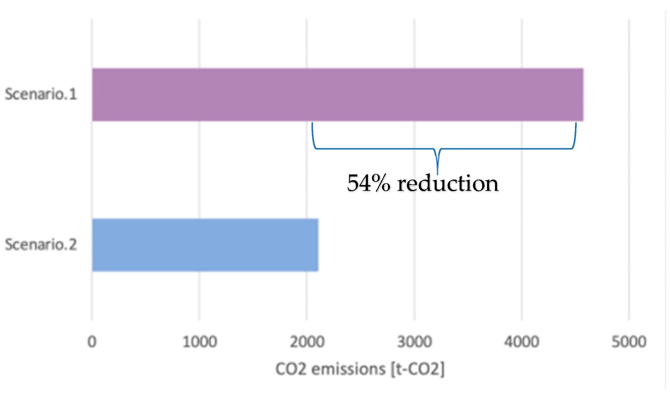
5.7. Comparison of CO2 Emissions with and without Bias
Figure 10 compares the carbon dioxide emissions of an unbiased logistics system (Scenario 1) and a biased logistics system (Scenario 2). The CO
2 emissions were calculated using the Simplified GHG Emissions Calculator published by the Environmental Protection Agency [
34] based on the total distance of the logistics system, the number of trucks, and the fuel consumption of the trucks. The results show that our proposed model (Scenario 2) achieves a 54% reduction in CO
2 emissions.
6. Conclusions
In this study, we present a novel GA-LKH model to optimize the location of logistics hubs and transportation routes in the PI framework by incorporating weighted region-specific flows. Another advantage of our model is that it employs real road maps provided by Google API. As an extension of the model proposed by Pan et al. [
5], our proposed model allows for more accurate optimization of logistics hubs, resulting in a significant reduction in CO
2 emissions by 54%.
Our study contributes to the field in four main ways. First, this study applies the concept of PI to the study of logistics networks. It addresses fundamental solutions to common global challenges in freight transportation, such as reducing greenhouse gas emissions, alleviating truck driver shortages, and improving profit margins in the transportation industry.
Second, this study extends the standard GA-LKH method proposed by Pan et al. [
4] to achieve improved performance without requiring new investment. To achieve this, this study incorporates weighted demographic information in each region into the model. In addition, we simulate the use of existing logistics centers as warehouses in conjunction with the concept of the PI, which allows optimization without additional investment. The application of the proposed model will help logistics companies improve their profitability.
Third, the simulation in this study uses real data. The research results were calculated by applying real-world GIS data, including factory locations, logistics hubs, and critical logistics roads to the proposed model. Therefore, the research results are both concrete and reliable. In addition, the model is scalable and can be applied to real data sets in other regions or countries for the solution of practical social problems in those areas.
Fourth, this study is also novel in that it optimizes routes using distance based on real roads, which includes actual traffic factors such as road type (expressways and general roads), vehicle type (gasoline, EV, hybrid, etc.), and traffic conditions in each section. This provides a more realistic approach than other delivery route optimization models by taking into account multiple factors that influence route selection.
In conclusion, this study proposes a more practicable model to simulate existing logistics hubs as shared logistics hubs in the context of the PI. The results of this study can be applied to real data in other regions and countries. This makes them highly valuable in the fields of urban logistics, PI implementation, and logistics sustainability.
The limitation of this paper is that it focuses on road transport optimization. Future research could explore the integration of different transportation modes and the use of real business data from logistics companies for real business needs.
Author Contributions
Conceptualization, H.N., E.H., N.F. and R.G.T.; methodology, H.N. and E.H.; software, H.N.; validation, E.H., N.F. and R.G.T.; data curation, H.N.; writing—original draft preparation, H.N. and E.H.; writing—review and editing, H.N., E.H., N.F. and R.G.T.; visualization, H.N.; supervision, E.H.; funding acquisition, E.H. All authors have read and agreed to the published version of the manuscript.
Funding
This work was supported by JSPS KAKENHI Grant Numbers JP 23K04076, JP 21H01564. This work was supported by the Initiatives for Diversity Research Environment project by the Ministry of Education, Sports, Science and Technology, and funded by Diversity Fund of Gender Equality Office, Inclusive Campus & Health Care Center, Kobe University.
Data Availability Statement
Publicly available data sets were analyzed in this study. These data can be found in related citations in the references.
Conflicts of Interest
The authors declare no conflicts of interest.
Appendix A
The pseudocode for the proposed model is presented below.
| Algorithm A1 Genetic Algorithm |
Define Genetic Algorithm Parameters:- -
N = 40 [Population size] - -
G = 100 [Max generations] - -
Rcross = 0.6 [Crossover rate] − Rmut = 0.01 [Mutation rate] − p = 1000 [Penalty coefficient] Define Gene Class: - -
Representing a configuration of locker locations.
Utility Functions:- -
calculate total distance(): Calculate total distance of a given route. - -
calculate route(): Calculate the optimal route using LKH-3. - -
evaluate fitness(): Evaluate the fitness of a gene based on various factors. - -
selection(): Selecting the top 10% of genes. - -
crossover(): Perform crossover between two parent genes. - -
mutate(): Apply mutation to a gene.
Genetic Algorithm Function:- -
genetic algorithm(): - -
Initialize a population of genes randomly. - -
Evaluate fitness of each gene. - -
Select parents using elitist preserving selection. - -
Perform crossover and mutation to create new genes. - -
Iterate for a specified number of generations. - -
Return the best gene found. Main Execution: - -
Execute the genetic algorithm. - -
Print the best gene and optimal route. - -
Obtain coordinates of selected locker locations. - -
Use LKH-3 to calculate the optimal route for genes.
|
References
- C2ES CO2 Emissions Which Accounts for about 76% of Greenhouse Gas Emissions—Google Search. Available online: https://www.c2es.org/content/international-emissions/ (accessed on 24 March 2024).
- McKinnon, A.C. Freight Transport Deceleration: Its Possible Contribution to the Decarbonisation of Logistics. Transp. Rev. 2016, 36, 418–436. [Google Scholar] [CrossRef]
- IRU Global Truck Driver Shortage Report 2023. Available online: https://www.iru.org/resources/iru-library/global-truck-driver-shortage-report-2023 (accessed on 23 March 2024).
- Montreuil, B.; Meller, R.D.; Ballot, E. Towards a Physical Internet: The Impact on Logistics Facilities and Material Handling Systems Design and Innovation. In Proceedings of the 11th IMHRC, Milwaukee, WI, USA, 21–24 June 2010; Volume 40. [Google Scholar]
- Pan, S.; Zhang, L.; Thompson, R.G.; Ghaderi, H. A Parcel Network Flow Approach for Joint Delivery Networks Using Parcel Lockers. Int. J. Prod. Res. 2020, 59, 2090–2115. [Google Scholar] [CrossRef]
- Treiblmaier, H.; Mirkovski, K.; Lowry, P.B. Conceptualizing the Physical Internet: Literature Review, Implications and Directions for Future Research. In Proceedings of the 11th CSCMP Annual European Research Seminar, Vienna, Austria, 12–13, May 2016; Available online: https://ssrn.com/abstract=2861409 (accessed on 24 March 2024).
- Pan, S.; Ballot, E.; Huang, G.Q.; Montreuil, B. Physical Internet and Interconnected Logistics Services: Research and Applications. Int. J. Prod. Res. 2017, 55, 2603–2609. [Google Scholar] [CrossRef]
- Münch, C.; Wehrle, M.; Kuhn, T.; Hartmann, E. The Research Landscape around the Physical Internet—A Bibliometric Analysis. Int. J. Prod. Res. 2023, 62, 2015–2033. [Google Scholar] [CrossRef]
- Simatupang, T.M.; Sridharan, R. The Collaborative Supply Chain. Int. J. Logist. Manag. 2002, 13, 15–30. [Google Scholar] [CrossRef]
- Ji, S.; Peng, X.; Luo, R. An Integrated Model for the Production-Inventory-Distribution Problem in the Physical Internet. Int. J. Prod. Res. 2019, 57, 1000–1017. [Google Scholar] [CrossRef]
- Kulkarni, O.; Dahan, M.; Montreuil, B. Resilient Hyperconnected Parcel Delivery Network Design Under Disruption Risks. Int. J. Prod. Econ. 2022, 251, 108499. [Google Scholar] [CrossRef]
- Achamrah, F.E.; Lafkihi, M.; Ballot, E. A Dynamic and Reactive Routing Protocol for the Physical Internet Network. Int. J. Prod. Res. 2023, 1–19. [Google Scholar] [CrossRef]
- Hettle, C.; Faugere, L.; Kwon, S.; Gupta, S.; Montreuil, B. Generating Clusters for Urban Logistics in Hyperconnected Networks—Google Search. In Proceedings of the International Physical Internet Conference, Virtual, 14 June 2021; pp. 1–10. [Google Scholar]
- Mohammed, A.; Govindan, K.; Zubairu, N.; Pratabaraj, J.; Abideen, A.Z. Multi-Tier Supply Chain Network Design: A Key towards Sustainability and Resilience. Comput. Ind. Eng. 2023, 182, 109396. [Google Scholar] [CrossRef]
- Hakimi, D.; Montreuil, B.; Sarraj, R.; Ballot, E.; Pan, S. Simulating a Physical Internet Enabled Mobility Web: The Case of Mass Distribution in France. In Proceedings of the 9th International Conference on Modeling, Optimization & SIMulation—MOSIM’12, Bordeaux, France, 6–8 June 2012; 10p. [Google Scholar]
- Ballot, E.; Montreuil, B. “Functional Design of Physical Internet Facilities: A Road-Rail Hub” by Eric Ballot, Benoit Montreuil et al. Available online: https://digitalcommons.georgiasouthern.edu/pmhr_2012/13/ (accessed on 4 December 2023).
- Ferrell, W.; Ellis, K.; Kaminsky, P.; Rainwater, C. Horizontal Collaboration: Opportunities for Improved Logistics Planning. Int. J. Prod. Res. 2020, 58, 4267–4284. [Google Scholar] [CrossRef]
- Fazili, M.; Venkatadri, U.; Cyrus, P.; Tajbakhsh, M. Physical Internet, Conventional and Hybrid Logistic Systems: A Routing Optimisation-Based Comparison Using the Eastern Canada Road Network Case Study. Int. J. Prod. Res. 2017, 55, 2703–2730. [Google Scholar] [CrossRef]
- Meller, R.D.; Montreuil, B.; Thivierge, C.; Montreuil, Z. Functional Design of Physical Internet Facilities: A Road-Based Transit Center. In Functional Design of Physical Internet Facilities: A Road-Based Transit Center; MHIA: Charlotte, NC, USA, 2012. [Google Scholar]
- Sarraj, R.; Ballot, E.; Pan, S.; Hakimi, D.; Montreuil, B. Interconnected Logistic Networks and Protocols: Simulation-Based Efficiency Assessment. Int. J. Prod. Res. 2014, 52, 3185–3208. [Google Scholar] [CrossRef]
- Chargui, T.; Bekrar, A.; Reghioui, M.; Trentesaux, D. Proposal of a Multi-Agent Model for the Sustainable Truck Scheduling and Containers Grouping Problem in a Road-Rail Physical Internet Hub. Int. J. Prod. Res. 2020, 58, 5477–5501. [Google Scholar] [CrossRef]
- Yang, Y.; Pan, S.; Ballot, E. Mitigating Supply Chain Disruptions through Interconnected Logistics Services in the Physical Internet. Int. J. Prod. Res. 2017, 55, 3970–3983. [Google Scholar] [CrossRef]
- Hosoda, J.; Irohara, T. Recent Research on Variants of the Location Routing Problem. J. Jpn. Ind. Manag. Assoc. 2022, 73, 75–91. [Google Scholar]
- Sluijk, N.; Florio, A.M.; Kinable, J.; Dellaert, N.; Van Woensel, T. Two-Echelon Vehicle Routing Problems: A Literature Review. Eur. J. Oper. Res. 2023, 304, 865–886. [Google Scholar] [CrossRef]
- Schneider, M.; Drexl, M. A Survey of the Standard Location-Routing Problem. Ann. Oper. Res. 2017, 259, 389–414. [Google Scholar] [CrossRef]
- Pelleg, D.; Moore, A.W. X-Means: Extending k-Means with Efficient Estimation of the Number of Clusters. In Proceedings of the International Conference on Machine Learning (ICML), San Francisco, CA, USA, 29 June–2 July 2000; Volume 1, pp. 727–734. [Google Scholar]
- Ishioka, T. An Expansion of X-Means: Progressive Iteration of K-Means and Merging of the Clusters. J. Comput. Stat. 2006, 18, 3–13. [Google Scholar]
- Helsgaun, K. An Extension of the Lin-Kernighan-Helsgaun TSP Solver for Constrained Traveling Salesman and Vehicle Routing Problems; Roskilde Universitet: Roskilde, Denmark, 2017; Volume 12. [Google Scholar]
- Dimitrovski, F. Elkai. Available online: https://pypi.org/project/elkai/ (accessed on 22 September 2023).
- MLIT National Land Information Download Site 2023. Available online: https://nlftp.mlit.go.jp/ksj/index.html (accessed on 22 September 2023). (In Japanese)
- MLIT Portal Site of Official Statistics of Japan. Available online: https://www.e-stat.go.jp/en (accessed on 22 September 2023).
- MLIT National Survey of Net Freight Flows (Logistics Census). Available online: https://www.mlit.go.jp/sogoseisaku/transport/butsuryu06100.html (accessed on 22 September 2023).
- Isuzu Products & Solutions. Head Quarter Location: 1-2-5, Takashima, Nishi-ku, Yokohama-shi, Kanagawa, 220-8720, Japan. Available online: https://www.isuzu.co.jp/world/product/ (accessed on 22 September 2023).
- EPA, O. Simplified GHG Emissions Calculator. Available online: https://www.epa.gov/climateleadership/simplified-ghg-emissions-calculator (accessed on 8 December 2023).
Figure 1.
Delivery flow. Dotted lines indicate potential flow routes, while solid black arrows indicate the chosen routes. Suppliers () and customers () are grouped into clusters, and their respective goods are transported through collection points , and distribution points .
Figure 1.
Delivery flow. Dotted lines indicate potential flow routes, while solid black arrows indicate the chosen routes. Suppliers () and customers () are grouped into clusters, and their respective goods are transported through collection points , and distribution points .
Figure 2.
Model procedures.
Figure 2.
Model procedures.
Figure 3.
Clustering using the fuzzy c-means method. (a) Clustering of customers (factory sites). Different colors represent different clusters. (b) Clustering of distributors (distribution centers). Different colors represent different clusters.
Figure 3.
Clustering using the fuzzy c-means method. (a) Clustering of customers (factory sites). Different colors represent different clusters. (b) Clustering of distributors (distribution centers). Different colors represent different clusters.
Figure 4.
Drawing on map (without bias). The black line represents the optimal route, the red dots represent suppliers, the red pins represent supplier cluster centers, the blue dots represent customers, the blue pins represent customer cluster centers, and the green pins represent logistics hubs.
Figure 4.
Drawing on map (without bias). The black line represents the optimal route, the red dots represent suppliers, the red pins represent supplier cluster centers, the blue dots represent customers, the blue pins represent customer cluster centers, and the green pins represent logistics hubs.
Figure 5.
Drawing on map (with bias). The black line represents the optimal route, the red dots represent suppliers, the red pins represent supplier cluster centers, the blue dots represent customers, the blue pins represent customer cluster centers, and the green pins represent logistics hubs.
Figure 5.
Drawing on map (with bias). The black line represents the optimal route, the red dots represent suppliers, the red pins represent supplier cluster centers, the blue dots represent customers, the blue pins represent customer cluster centers, and the green pins represent logistics hubs.
Figure 6.
Adaptability of the GA for different population sizes.
Figure 6.
Adaptability of the GA for different population sizes.
Figure 7.
Execution time for different population sizes.
Figure 7.
Execution time for different population sizes.
Figure 8.
Execution time per generation (population size = 40).
Figure 8.
Execution time per generation (population size = 40).
Figure 9.
Transport routes along actual roads (with bias).
Figure 9.
Transport routes along actual roads (with bias).
Figure 10.
Comparison of CO2 emissions for two scenarios.
Figure 10.
Comparison of CO2 emissions for two scenarios.
Table 1.
Number, gross floor area, and estimated capacity of warehouses in Japan (2019–2022).
Table 1.
Number, gross floor area, and estimated capacity of warehouses in Japan (2019–2022).
| Year | Number of Buildings | Total Floor Space (m2) | Total Floor Area (m2) | Height (m2) | Utilization Rate | Capacity (m3) |
|---|
| 2019 | 14,728 | 10,025,455 | 6,807,071,564 | 5.5 | 40% | 1498 |
| 2020 | 14,953 | 11,862,478 | 7,933,175,951 | 5.5 | 40% | 1746 |
| 2021 | 13,469 | 13,386,200 | 9,938,525,503 | 5.5 | 40% | 2187 |
| 2022 | 12,995 | 12,813,397 | 9,860,251,635 | 5.5 | 40% | 2170 |
| Average | 14,036 | 12,021,883 | 8,634,756,163 | 5.5 | 40% | 1900 |
Table 2.
Estimated truck capacity.
Table 2.
Estimated truck capacity.
| Type | Width (mm) | Length (mm) | Height (mm) | Capacity (m2) | Car Model |
|---|
| Light-duty trucks (2 t) | 1620 | 3120 | 2330 | 12 | ELF |
| Medium trucks (4 t) | 2230 | 6225 | 2400 | 34 | FORWARD |
| Heavy trucks (10 t) | 2410 | 9675 | 2500 | 59 | GIGA G-CARGO |
Table 3.
Parameters for the GA.
Table 3.
Parameters for the GA.
| Name | Value |
|---|
| Population size | 40 |
| Max generations | 100 |
| Crossover rate | 0.8 |
| Mutation rate | 0.01 |
| Penalty coefficient | 100 |
| Maximum number of logistics nodes | 25 |
| Disclaimer/Publisher’s Note: The statements, opinions and data contained in all publications are solely those of the individual author(s) and contributor(s) and not of MDPI and/or the editor(s). MDPI and/or the editor(s) disclaim responsibility for any injury to people or property resulting from any ideas, methods, instructions or products referred to in the content. |
© 2024 by the authors. Licensee MDPI, Basel, Switzerland. This article is an open access article distributed under the terms and conditions of the Creative Commons Attribution (CC BY) license (https://creativecommons.org/licenses/by/4.0/).


