Abstract
Background: Integrating artificial intelligence in unmanned aerial vehicle systems may enhance the surveillance process of outdoor expansive areas, which are typical in logistics facilities. In this work, we propose methods to optimize the training of such high-performing systems. Methods: Specifically, we propose a novel approach to tune the training hyperparameters of the YOLOv3 model to improve high-altitude object detection. Typically, the tuning process requires significant computational effort to train the model under numerous combinations of hyperparameters. To address this challenge, the proposed approach systematically searches the hyperparameter space while reducing computational requirements. The latter is achieved by estimating model performance from early terminating training sessions. Results: The results reveal the value of systematic hyperparameter tuning; indicatively, model performance varied more than 13% in terms of mean average precision (mAP), depending on the hyperparameter setting. Also, the early training termination method saved over 90% of training time. Conclusions: The proposed method for searching the hyperparameter space, coupled with early estimation of model performance, supports the development of highly efficient models for UAV-based surveillance of logistics facilities. The proposed approach also identifies the effects of hyperparameters and their interactions on model performance.
1. Introduction
Logistics hubs, including ports, are key links to modern supply chains. In these hubs, logistics service providers collaborate to transship among multiple modes, store goods and offer value-added services through asset and operations sharing, taking advantage of economies of scale. One significant aspect of logistics hubs is security against a wide array of threats, including unauthorized entry, cargo theft, illicit trade and terrorism. Cargo owners and logistics providers have long recognized that guarding against security threats is fundamental to business continuity, operational efficiency and cost-effectiveness [1]. As a result, logistics hubs have developed strong practices, processes and systems that are security-certified under international standards, such as the ISPS code [2] or TAPA [3]. Among others, these standards focus on access processes and restrictions and the means to raise alarms against illegal activities through surveillance.
To effectively address these areas, it is beneficial to include advanced technology systems in the logistics hub security strategy [1,4]. The industry status with respect to surveillance requirements, operations and systems has been reviewed in [5], indicating that logistics facility operators use mostly traditional surveillance systems, such as Closed-Circuit TV (CCTV). In this case, a set of surveillance cameras are installed throughout the facility and provide real-time video feed to the operator(s) responsible for monitoring potential suspicious activity. The requirement of human supervision, however, may pose challenges related to reliability and costs [6]. Furthermore, the efficiency and efficacy of the CCTV set-up are not ideal due to the large physical space the facility extends to [7]. Finally, CCTV cameras have a specific field of view, and, as a result, blind spots cannot be avoided [8].
Thus, users agree that more advanced systems are necessary to eliminate the weaknesses of CCTV-based systems [5]. In response to this need, the industry is shifting towards integrating UAVs into surveillance operations [9]. Drone-based surveillance systems offer superior coverage and efficiency. Integration of AI in such systems enables drones to accurately track objects and autonomously identify potential threats with minimal human intervention, enhancing the reliability of surveillance operations [10].
The YOLOv3 model, a one-stage artificial intelligence object detector, has been shown to be highly effective for drone-based surveillance systems due to its fast and precise object detection and recognition capabilities. It may locate an object and determine its class in real time, which is essential in dynamic aerial supervision situations [11]. Furthermore, YOLOv3 may detect small objects, which is an important requirement for drones that operate in various and demanding conditions, such as diverse and oftentimes high altitudes and variable lighting conditions [12].
However, training YOLO AI models is a complex process that requires extensive annotated data, in many cases from several sources [13]. It also requires significant computer resources [14]. There are additional training challenges for drone imaging object detection: UAV photos have low resolution, and this frequently results in the blurring of objects. Several object categories may also be underrepresented in drone images, and object sizes may vary over a broad range due to the angle and height of the drone [15]. These variations necessitate the use of highly robust algorithms. Finally, it is worth noting the scarcity of drone-specific datasets, which may affect the effectiveness of training.
The purpose of this study is to optimize the training of the YOLOv3 object detection model to effectively support drone surveillance systems operating in logistics hubs and facilities. Specifically, we aim to tune the model’s hyperparameters to achieve superior training for high-altitude object detection in outdoor environments that are typical of logistics hubs. The main challenge is the computational time and resources required for experimenting with a large number of hyperparameter combinations during training. To accelerate this process, we have explored two levers: (a) how to systematically search the hyperparameter space and (b) how to minimize the training time required to assess each hyperparameter combination. For the first lever, we employ a full factorial design of experiments (DOE) to explore the space of hyperparameters. For the second lever, we estimate model performance for each hyperparameter combination early in the training process, thus considerably reducing the hyperparameter tuning process.
The structure of the remainder of this paper is as follows: Section 2 overviews important research on drone surveillance systems that incorporate AI. Section 3 outlines the method for hyperparameter tuning. Section 4 presents the analysis of the factorial experiments and estimates the effects of hyperparameters on model performance. Section 5 discusses an early termination strategy to reduce the computational time in hyperparameter space exploration. In Section 6, we validate the performance of the tuned YOLOv3 model and the proposed early termination strategy. Finally, Section 7 presents the conclusions of the study, discusses key aspects of the proposed approaches and proposes directions for future research.
2. Background
2.1. Surveillance Through AI-Powered UAVs
UAVs equipped with cameras and on-board CPUs offer the flexibility to efficiently survey expansive areas, thereby mitigating the limitations of static cameras. These aerial devices can perform real-time video processing and utilize AI to detect suspicious activity [9]. In such cases, object location and classification information, as well as the related video streams, can be automatically sent to security teams to take prompt action [16]. The deployment of UAV surveillance systems requires advanced computational capabilities coupled with robust and fast algorithms that can identify suspicious activity.
Singh Amarjot et al. [17] propose a two-stage approach to address the related challenges. The first stage employs a Feature Pyramid Network (FPN) [18] to detect humans in live aerial footage. This network is made up of two pathways: a top-down one that improves resolution by up-sampling feature maps and a bottom-up pathway that extracts standard features through convolutional layers. The two pathways are combined to enhance object identification in regions of interest that overlap. In the second stage, the human posture is assessed using the ScatterNet Hybrid Deep Learning (SHDN) model. The latter combines a regression network back-end with a ScatterNet front-end, which may extract complicated patterns and edge characteristics. As shown in [19], edge feature extraction is particularly relevant when examining different human positions in aerial photography.
Sahin and Ozer [20] introduced YOLODrone, an enhanced version of the standard YOLO architecture designed specifically for drone imagery. YOLODrone includes more detection layers and convolutional layers, resulting in improved detection of smaller and variably sized objects that are common in aerial images.
Jadhav et al. [21] utilize the YOLOv4 model and demonstrate improved detection and localization of objects, specifically vehicles, in restricted areas. The research showcases YOLOv4′s capability of working with low-resolution images (as low as 20 × 20 pixels) in practical applications that involve aerial surveillance.
Tan et al. [22] present an enhancement to the YOLOv4 algorithm, specifically optimized for drone imagery. This advancement addresses the challenges of detecting small and obstructed targets against complex backgrounds typical to UAV images. The modified YOLOv4_Drone incorporates a Receptive Field Block (RFB) module to resample feature maps and an Ultra-Lightweight Subspace Attention Mechanism (ULSAM) for multi-scale feature representation, improving feature extraction and detection accuracy. Additionally, the integration of a Soft Non-Maximum Suppression (Soft-NMS) process minimizes missed detections due to target occlusion. Experimental results demonstrate a 5% improvement in detection accuracy over the standard YOLOv4 [22].
Recent advances have made it possible for processing to be carried out on-board UAVs through the integration of robust and lightweight computing devices [9]. The right balance between processor speed, application efficiency, weight and size of computing hardware has been a central point in real-time UAV applications. DroNet, by Kyrkou et al. [23], uses a deep CNN detector for real-time UAV applications. The DroNet architecture is characterized by a single-shot CNN model consisting of 14 layers: nine convolution layers, four max-pooling layers and a dedicated decode-detect layer [23]. DroNet’s performance is benchmarked against various models, such as small YOLOv3, Tiny YOLO and Tiny YOLONET. The model was implemented on a DJI Matrice 100 UAV, using single-board platforms, such as Odroid Xu4 and Raspberry Pi 3. DroNet achieved 95% detection accuracy at 8–10 frames per second (FPS) on the Odroid Xu4 hardware and the same level of accuracy at 5–6 FPS on Raspberry Pi 3 [23].
Benhadhria et al. [24] developed VAGADRONE, a fully autonomous system integrating board the UAV a Raspberry Pi 3, which uses Android 9 to enable effective navigation, live streaming and data processing. The design incorporates a Camera Serial Interface (CSI) for direct video recording onto the SD card of the Raspberry Pi, as well as a smart card reader for 4G connectivity, which enables high-speed internet access for live video streaming [24]. VAGADRONE has been tested in applications that include object identification, face recognition and object counting [24].
2.2. Research Relevant to the Methods Proposed in This Work
Beyond UAV-based object identification and real-time processing, AI techniques have also been adopted in other intrusion identification applications, such as cybersecurity. For example, Ashraf et al. [25] propose an intrusion detection strategy (IDS) for wireless sensor networks (WSNs) using machine learning techniques to detect and mitigate denial-of-service (DoS) attacks such as Grayhole, Blackhole, Flooding and TDMA. The study evaluates five classification models, K-Nearest Neighbors (KNN), Naïve Bayes, Logistic Regression, Support Vector Machine (SVM) and Artificial Neural Networks (ANN), on a large dataset collected via the LEACH protocol, achieving intrusion detection accuracy up to 98%.
There has also been interesting research work using the design of experiments (DOE) for hyperparameter tuning. Lee et al. [26] applied a multi-level factorial design to optimize YOLOv3 training for single-class license plate detection. Their study revealed both main and up to two-way interaction effects between hyperparameters. Firstly, they explored three hyperparameters and selected the best-identified levels for the ones that were statistically significant. The second stage explored three additional parameters and treated them in the same fashion. Chen et al. [27] applied a simple experimental design to optimize hyperparameters for a binary smoke detection task (smoke vs. no smoke). Their study primarily focused on analyzing the main effects without conducting ANOVA and assessing statistical significance. No hyperparameter interactions have been studied.
In other related work, researchers adjust the default values of training hyperparameters based on the target dataset and application requirements [28]. For example, the default hyperparameters of YOLOv5, including learning rate, momentum, weight decay, etc., have been optimized through previous experimentation and incorporated into the model. Hou et al. [29] proposed a YOLOv5s-based tuning scheme for target detection in complex underwater environments. They applied hyperparameter evolution using a genetic algorithm to optimize 29 key parameters such as learning rate, momentum and weight decay, achieving a 4.5% increase in mAP compared to the original YOLOv5s model. Note that the GA approach may not reveal the effects of the hyperparameters and their interactions on training performance.
2.3. This Current Research Work
Our review of the literature reveals opportunities for further enhancing the training performance of AI-powered UAV surveillance systems. Specifically, an area of significant promise is the systematic and efficient tuning of training hyperparameters to optimize the performance of the trained model. The current study makes two contributions toward this end with respect to the state of the art:
First, we propose a method to systematically explore the space of training hyperparameters and identify (a) the effects of each hyperparameter and of all possible hyperparameter interactions on the performance of the trained model in object identification (through mAP), as well as (b) the most effective combination of hyperparameter levels for model training (among the levels that were tested).
Second, to address the computational time challenge, our research proposes an approach to predict the performance of a model at an early stage of training. Thus, the computational time to assess the merit of each hyperparameter combination is significantly reduced, and the practicality of the proposed search method is considerably strengthened.
With respect to the existing literature, both contributions are novel. For the first contribution, our work applies DOE to a multi-class object detection task in a complex and dynamic environment involving UAV-based surveillance. Unlike previous studies, our approach explores both main and higher-order interaction effects, providing a more comprehensive understanding of hyperparameter effects on training. The second contribution related to estimating model performance from early training stages is also novel with respect to the current literature.
3. The Method for Hyperparameter Tuning
3.1. Method Overview
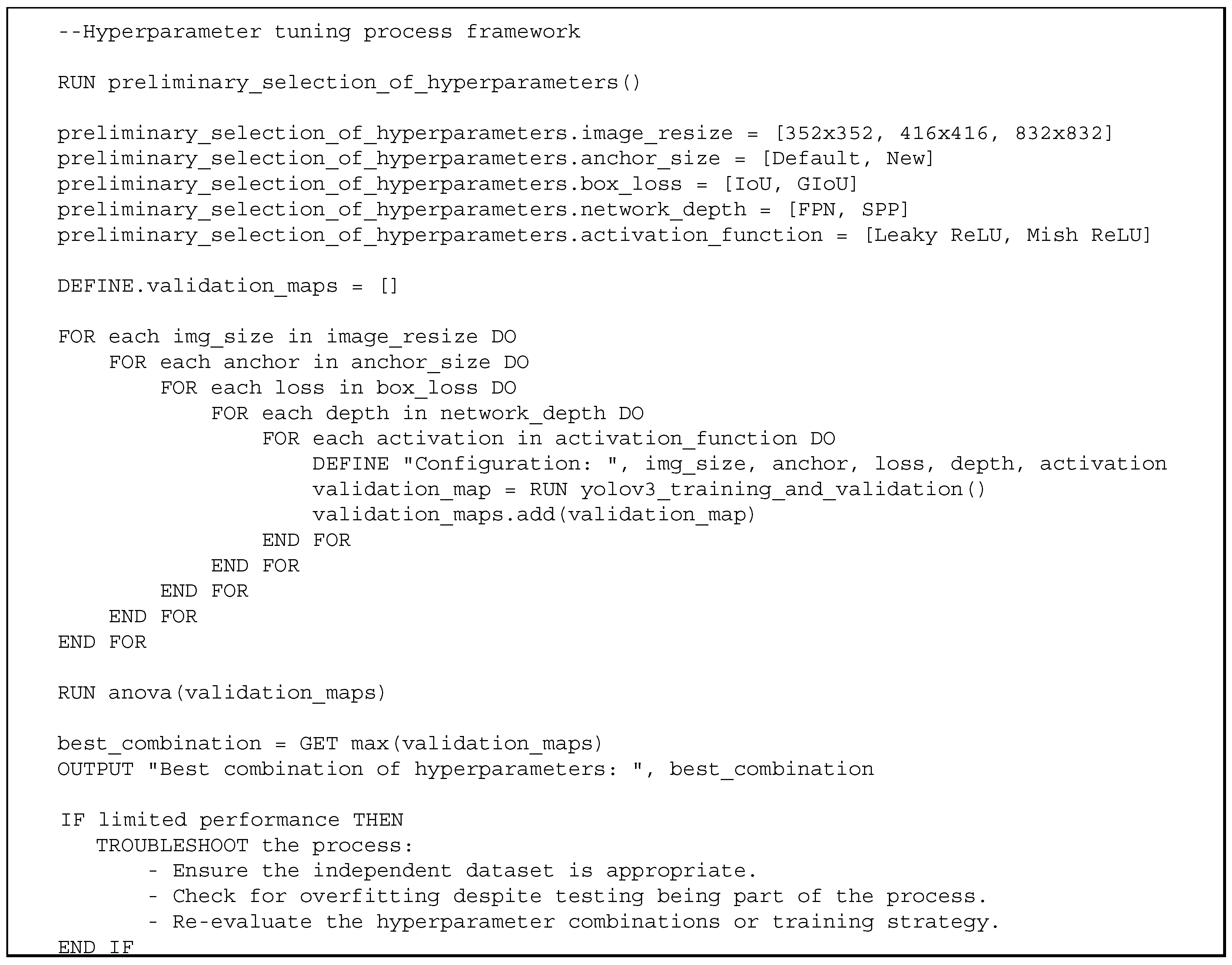
The methodological framework to address the objectives of (a) systematic exploration training hyperparameter space and (b) reduction in training time to make this exploration computationally feasible includes the following steps (see Figure 1):
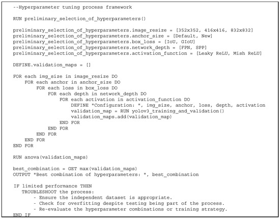
Figure 1.
Hyperparameter tuning process framework in pseudocode.
- Select the training hyperparameters and their levels to explore. This can be performed based on experience, expert knowledge or a preliminary experimental study.
- Conduct full factorial experiments; that is, train and test the models developed under all combinations of hyperparameters. Confirm the absence of overfitting through the testing dataset. Note that the experimental process should provide an adequate estimation of the mAP variance required for ANOVA. For this reason, it is recommended that each experiment be performed twice.
- For computational effectiveness, use the early termination method proposed in this manuscript.
- Perform the ANOVA analysis to identify the effects of significant hyperparameters and hyperparameter interactions on mAP.
- Identify the best combination of hyperparameters.
- Confirm that the model trained under this hyperparameter combination performs well in independent datasets. If performance is limited, troubleshoot the process (e.g., ensure the independent confirmation dataset is appropriate, examine if overfitting has occurred in the training process despite the testing being performed as part of the process, etc.).
Below, we first overview the YOLOv3 algorithm and the dataset selected for training. Subsequently, we discuss key hyperparameters that affect the performance of the trained model. Finally, we present the factorial experiments used to evaluate the effects of selected hyperparameters and their interactions on performance. The approach for reducing training time is elaborated further in Section 5.
3.2. The YOLOv3 Algorithm and the Training Dataset
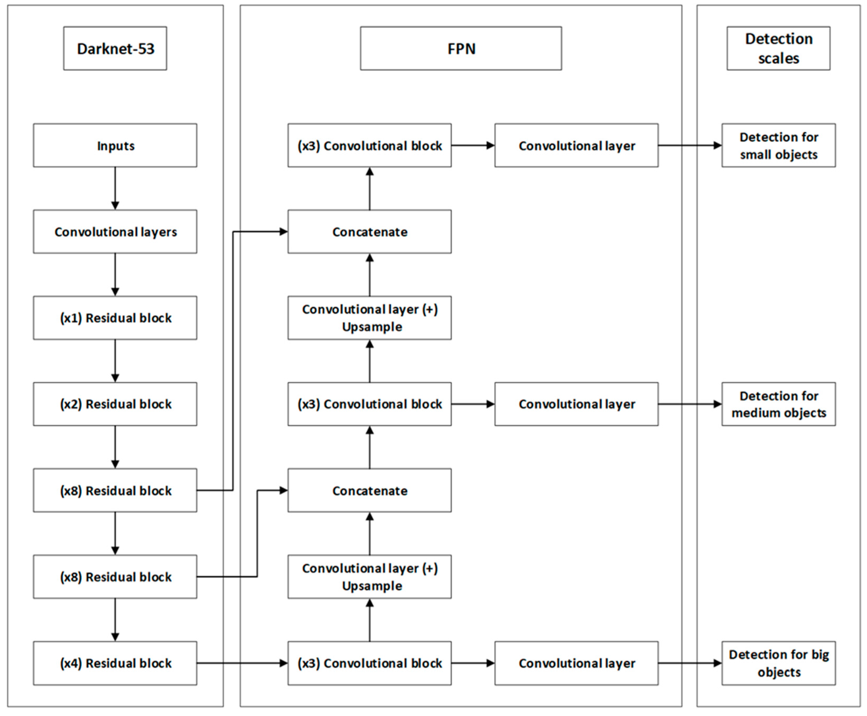
YOLOv3 is an object detection algorithm well-known for its efficiency and accuracy in real-time applications. Introduced by Redmon and Farhadi in 2018, it improves upon its predecessors, YOLO and YOLOv2, by enhancing the detection of a wider variety of objects with higher precision [30]. The architecture of YOLOv3 is depicted in Figure 2 and consists of several components that work together to efficiently detect objects.
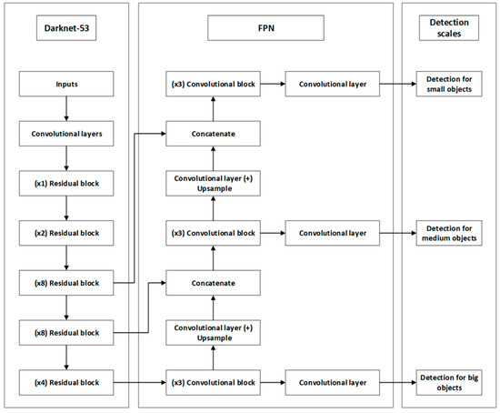
Figure 2.
YOLOv3 architecture.
Darknet-53 acts as the backbone for feature extraction, consisting of convolutional layers and multiple residual blocks designed to prevent the loss of gradient information during training. The multipliers, such as (×1), (×2), (×4) and (×8), represent the times that learning structures are repeated in order to enhance the depth of the network and its feature recognition capabilities [30].
In addition to the backbone, the architecture of YOLOv3 contains the Feature Pyramid Network (FPN), which is essential in combining semantic information at different scales. It merges deeper, lower-resolution features with shallower, higher-resolution features through a series of upward sampling and merging steps [18].
The last part of the architecture includes the detection heads that are responsible for object detection tasks. These heads are specialized in different object sizes—small, medium and large—allowing the network to adapt its prediction capabilities based on the dimensions of the objects, optimizing both accuracy and processing efficiency [30].
For further information on YOLOv3, the reader may refer to [31,32,33].
To train YOLOv3 for the purposes of our research, we utilized the VisDrone-DET dataset (see example in Figure 3) [34], which was specially created for training object identification models in images taken from unmanned aerial vehicles (UAVs). The dataset was chosen for its wide-ranging variety of aerial photos that contain persons and vehicles, among other objects. Specifically, it consists of 10,209 photos (images) taken in urban and rural areas with a total of 457,066 annotated objects.
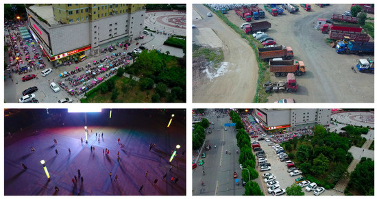
Figure 3.
Annotated sample images in the VisDrone-DET dataset [34].
VisDrone-DET has been split into four subsets to support different stages of model training and evaluation:
- Training set: Consists of 6471 images;
- Validation set: Consists of 548 images for periodic evaluation and tuning of model parameters during training;
- Test—development: Includes 1610 images used for final model evaluation before deployment;
- Test—challenge: Contains 1580 images for comparing model performance under competition conditions.
3.3. Training Hyperparameters
Certain hyperparameters manage the training process of YOLOv3 and, in turn, affect the performance of the trained model. These hyperparameters can be grouped into three main categories: Optimization-related, model architecture-related and detection performance-related (see Table 1).

Table 1.
Overview of training hyperparameters and their role in YOLOv3 training.
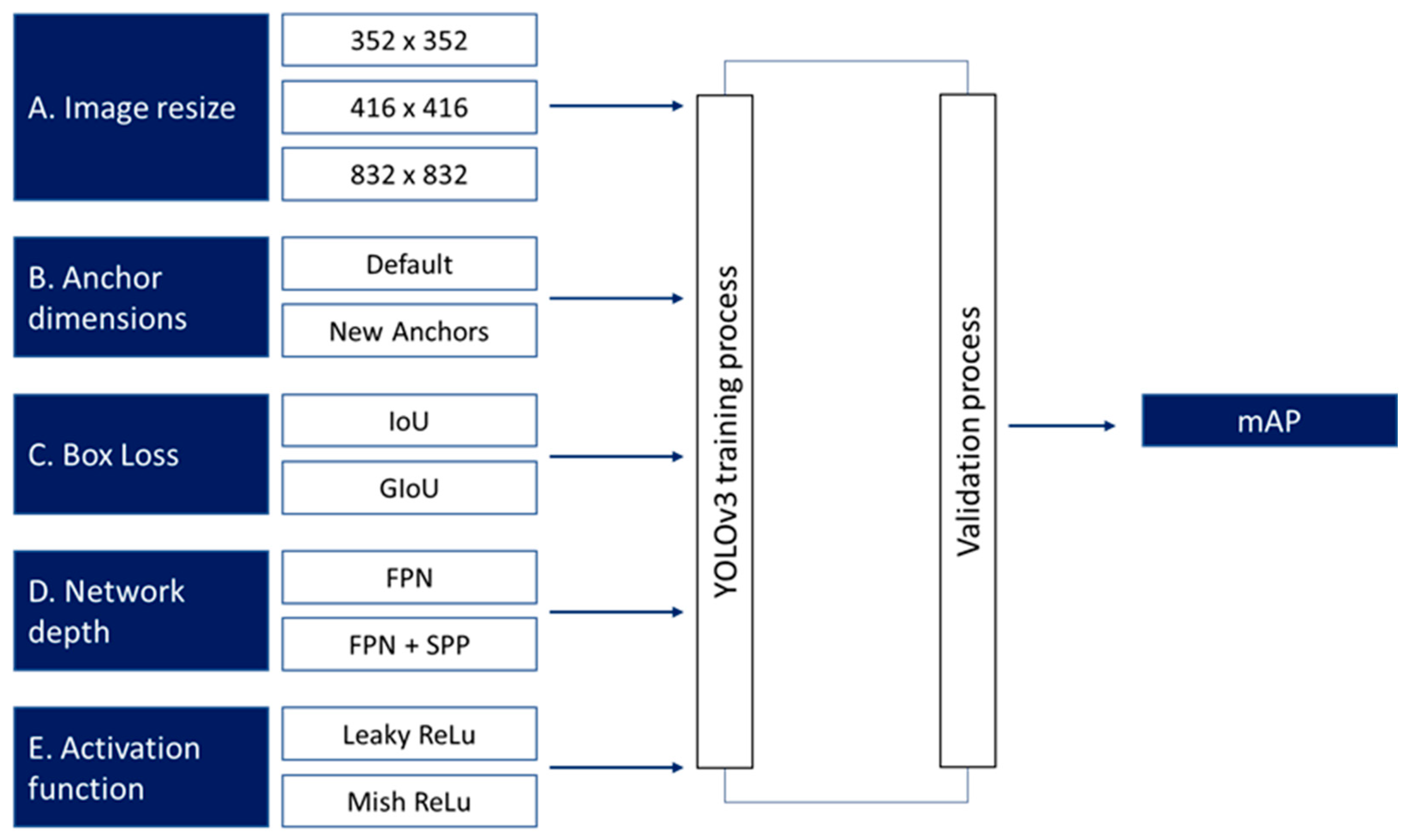
Related research [49,50,51,52] identified which hyperparameters have the most impact on object detection performance. Commonly tuned hyperparameters in YOLO, Faster R-CNN, SSD and other object detection models include learning rate, batch size, anchor box dimensions, image resolution, optimizer type, Intersection over Union (IoU) threshold, activation function and box loss. Other parameters may also be considered depending on the specific application and model architecture. To select the hyperparameters to focus on in the current work, we reviewed the relevant research [41,43,46,53,54], conducted preliminary experimentation to confirm the more relevant literature results and selected five influential hyperparameters among the ones studied (see Figure 4).

Figure 4.
Optimization parameters and their values for training the YOLOv3 model.
As shown in Figure 4, we defined three distinct levels for image resize and two levels for the other four hyperparameters. (Note that all five are commonly adjusted in similar research contexts; see [38,41,46,47,55].)
A few comments on the selected hyperparameters:
By varying the image dimensions {352 × 352, 416 × 416, 832 × 832}, we attempt to study the trade-off between training speed and detection accuracy. Smaller image sizes promote efficiency, while larger image sizes enhance detail and, thus, model performance.
Adjusting the dimensions of the anchor box (from the default) to ones that match the training dataset better makes it easier for the model to match the shapes and sizes of objects in the image; thus, training may become more efficient, and the model more precise.
Intersection over Union (IoU) measures object detector accuracy by comparing the overlap between predicted and ground truth boxes with respect to the area of their union. An advanced version, Generalized Intersection over Union (GIoU), unlike IoU, also considers the area of the smaller enclosing box, which contains both the predicted and ground truth box. As a result, GIoU measures not only the overlap but also the distance (closeness) between the boxes. This attempts to penalize incorrect predictions more effectively, potentially speeding up training [47].
The integration of depth networks such as FPN (Feature Pyramid Network) and FPN + SPP may also enhance feature extraction capabilities. These architectures utilize multi-scale information, with FPN merging different resolution features to create richer feature maps. The SPP module pools features at various scales, improving the model’s ability to maintain detailed features without extra computational costs [56].
The transition from Leaky ReLU to Mish ReLU may improve the learning process by providing more efficient gradient updates.
To assess model performance under different hyperparameter settings, we used the mean average precision (mAP) metric computed during the validation phase of model training. The mAP metric provides a comprehensive measure of model accuracy. It averages the detection precision of objects (a) across all classes and (b) at 11 recall levels (from 0 to 1). Note that precision refers to the percentage of true positives among all positive detections (including both true positives and false positives), while recall measures the percentage of true positives over the total number of objects that should have been detected (true positives plus false negatives) [57].
The mAP metric in the validation phase (validation mAP) provides a good estimation of how the model is expected to perform on unseen data without the potential risks of overfitting and underfitting associated with the training data. It also allows for iterative hyperparameter adjustments based on objective performance criteria.
3.4. Exploration of Hyperparameter Space
To adequately explore the space spanned by the five hyperparameters under study, we used a full factorial design of 48 (=24 × 3) hyperparameter combinations. Each combination was tested twice in order to quantify the variability within groups (and compare it to the variability among groups). The related analysis was performed by ANOVA.
Outside the experimental inputs of Figure 4, all other training hyperparameters were kept invariable throughout all experiments. However, the values of these hyperparameters were adjusted in the configuration file of YOLOv3 to fit the characteristics of the UAV dataset (see Table 2). In particular, the adjusted values reflect the reduction in the default number of classes (80) to the 10 classes in the present study.
Table 2.
Invariant hyperparameter settings: default vs. adjusted values.
It should be noted that the proposed method applies to any superset of hyperparameters that affect training and, subsequently, model performance considerably.
4. Experimental Results and Analysis
The computer system used for the experiments was equipped with an AMD Ryzen 9 3900X 12-Core Processor with 32GB RAM (Advanced Micro Devices, Inc., Santa Clara, CA, USA) and Nvidia RTX 3090 24GB graphics card (Nvidia Corporation, Santa Clara, CA, USA) with included CUDA and CuDNN drivers. Additionally, the OpenCV toolkit, an open-source computer vision library providing a wide range of tools for image and video processing, was installed and used in a variety of ways in the YOLOv3 model. Finally, to automatically adjust all the aforementioned hyperparameters, a Python script (version 3.10) was developed to guide the appropriate configuration of the YOLOv3 model across all experimental runs.
It is noted that YOLOv3 training needs significant computational resources, which lead to long computational times, especially when a less powerful system, such as the one above, is employed. Table 3 presents the effect of image dimensions on the computational time required to complete each training run using the above system. It is observed that the computational time increases almost linearly with the dimension of the image size.
Table 3.
Computational time required for a single combination of hyperparameters under different image resize settings.
4.1. Results and Analysis
The analysis of the experimental results (96 mAP values) was performed using MiniΤab software. Table 4 presents the significance of the effects and their interactions (p-value ≤ 0.05) on validation mAP. All main effects are statistically significant, as expected. Some two-way and three-way interactions are also significant, suggesting complex dependencies between the hyperparameters that affect the detection capabilities of the model. Only the significant interactions are shown in Table 4.
Table 4.
Statistically significant factors and factor interactions.
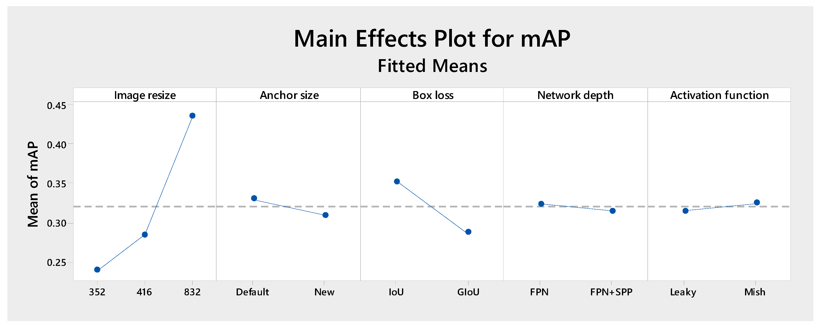
Figure 5 quantifies the effects of the main factors on the mAP:
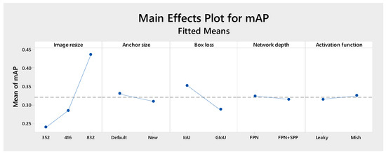
Figure 5.
Impact of various hyperparameters on validation mAP in YOLOv3. The blue line represents the effect of each factor level on the mean mAP, while the dashed line indicates the mean mAP.
- Image resolution affects mAP significantly since downsizing the image resolution from 832 × 832 to 416 × 416 and 352 × 352 yields mAP values of 45%, 30% and 25%, respectively. This is an expected finding for drone surveillance operating at high altitudes. In this case, objects generally occupy a few pixels in the image, and therefore, increased resolutions help in object detection by providing a larger number of pixels per object.
- Box loss analysis also affects model performance significantly. Using Intersection over Union (IoU) as compared to the Generalized IoU (GIoU) yields an increase in mAP of about 6%. This improvement shows that IoU provides better alignment between predicted and actual object boundaries compared to GIoU.
- The size of the anchor boxes has a less (but still statistically significant) impact on mAP, with a decrease of about 2% when changing from the default to the new anchor size.
- Network depth and activation functions show an even less (but still statistically significant) effect on mAP. Switching from a Feature Pyramid Network (FPN) to a Feature Pyramid Network with an added Spatial Pyramid Pooling (SPP) block, as well as changing the activation function from Leaky ReLU to Mish ReLU, yield a change in mean average precision (mAP) about 1%.
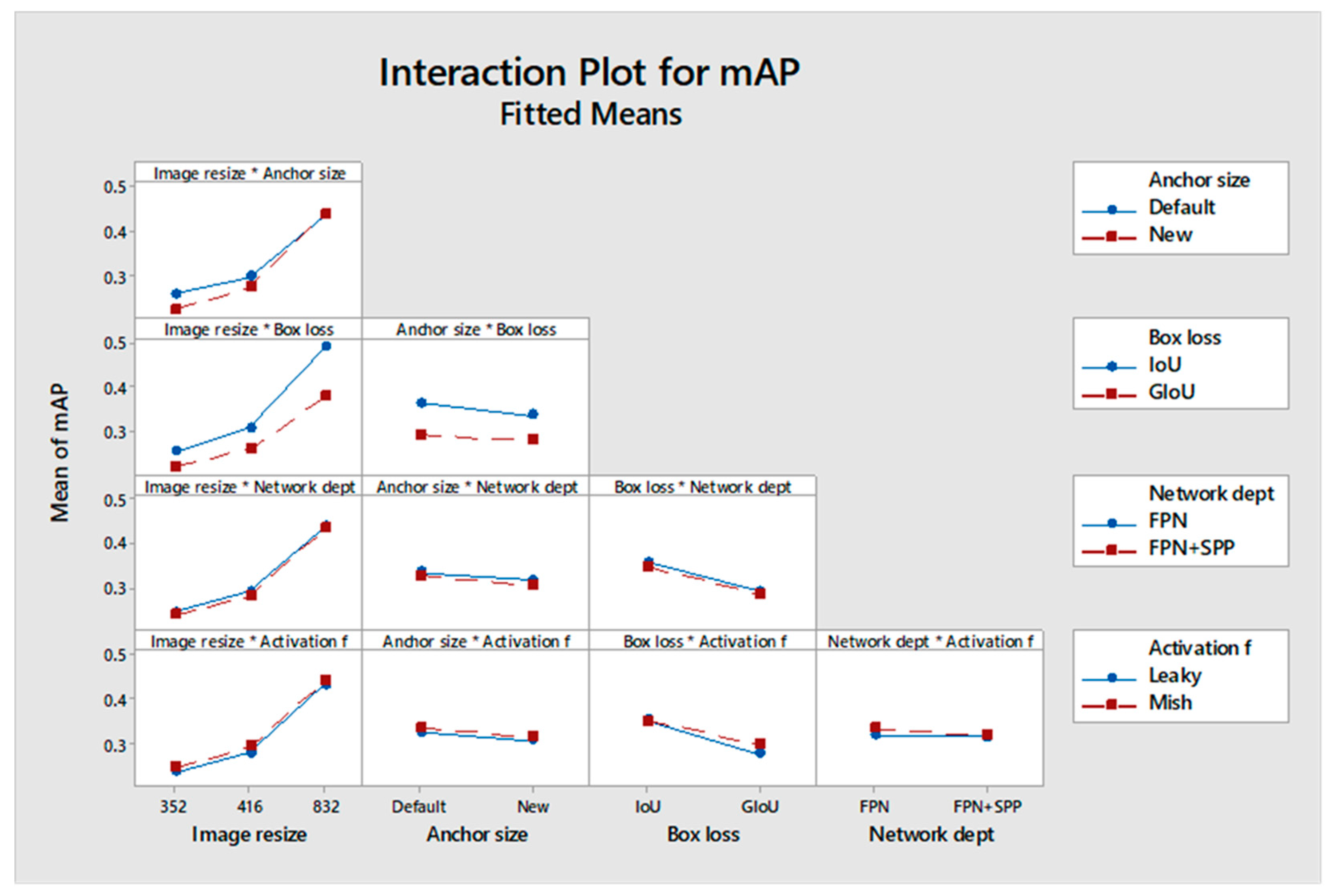
Figure 6 shows the two-way interaction effects on validation mAP. Consider, for example, the effect of the interaction between “Image resize” and “Anchor size”. The top left plot shows the mAP values at three different image resolutions, 352 × 352, 416 × 416 and 832 × 832, with two anchor size settings: the YOLOv3 default and an updated “new” anchor size. As the image resolution increases, mAP improves for both anchor settings, but the rate of improvement is steeper with the new anchor size than with the default. Therefore, for higher image resolutions, the effect of image resize on mAP is less important. The contrary is true for the interaction between image resize and box loss. The effect of box loss is more pronounced at high image resize levels. In general, two non-parallel curves in a plot indicate significant interactions.
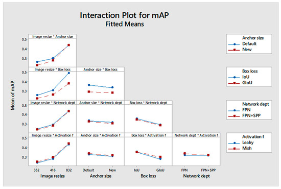
Figure 6.
Interaction effects on the validation mAP across different hyperparameter combinations in YOLOv3 model training. The asterisk (*) represents the interaction between hyperparameters.
The optimal hyperparameter combination that reached the highest mAP of 50.33% is achieved by resizing the image to 832 × 832, using default anchor sizes, Intersection over Union (IoU) for box losses, Feature Pyramid Network (FPN) for network depth, and Leaky ReLU as an activation function. This configuration excels due to the 832 × 832 resolution that enhances feature detail, while the default anchor sizes probably match well with the typical object scales in the UAV dataset. IoU box loss effectively balances accuracy and recall, FPN incorporates semantic information at all scales, improving detection capabilities, and Leaky ReLU maintains active neurons, ensuring consistent learning throughout the network.
4.2. Robustness of the Method with Respect to Datasets and Network Architecture
To verify the robustness of our hyperparameter tuning approach in terms of input data, we have conducted related experiments and analysis (ANOVA) on the mAP results produced from two datasets: (a) the training/validation one and (b) the testing one. That is, the effects of the hyperparameters and their interactions on mAP were estimated twice based on two independent (but related) datasets. The analysis resulting from these two datasets indicated very similar effects of the main factors and factor interactions on mAP. For example, the total effect of image resize from the validation dataset analysis was estimated to be 20%, and from the test dataset analysis was 15%. Similar results were obtained from the analysis of the two datasets regarding anchor size (2% vs. 1.4%), box loss (6% vs. 4%), network depth (1% vs. 0.4%) and activation function (1% vs. 0.4%), as well as for the factor interactions.
A second investigation in terms of robustness across input datasets, included verification experiments using the DeOPSys dataset, a custom and totally independent dataset related to logistics hub surveillance. The results were very encouraging (see Table 7 of Section 6 below), confirming once more the applicability and robustness of the method across datasets.
In terms of the robustness of network architectural changes, the YOLOv3 architecture was one of the factors tested in our work. In particular, we tested two model architectures. The first is YOLOv3 with Feature Pyramid Network (FPN), and the second is YOLOv3 with FPN + Spatial Pyramid Pooling (SPP) module. The effect (difference) on the mAP of these two architectures is limited but statistically significant (see Table 4 and Figure 4 of the manuscript under network depth). Similar outcomes hold for the interaction of network depth with other factors. ANOVA analysis related to the FPN vs. the FPN+SPP outcomes (two separate analyses, one per architecture) confirmed that the main effects of image resize (19.5% vs. 19.8%), anchor size (1.8% vs. 2.2%), box loss (6.8% vs. 6.1%) and activation function (1.4% vs. 0.5%) are statistically significant and similar in both FPN and FPN+SPP architectures. The same holds for the factor interactions, indicating the robustness of the analysis across network architectures.
Regarding the training time technique, in the validation case, the best configuration with the FPN architecture using the early termination method is 0.8% away from the best FPN configuration obtained through exhaustive training, while the best configuration with the FPN + SPP architecture is 1.7% away. Similar results were obtained from the VisDrone and DeOPSys test datasets. These differences are limited, indicating that the early termination method effectively identifies high-performing configurations under both architectures tested.
4.3. A Note on Overfitting Avoidance and Computational Effort
In this study, overfitting avoidance was tested in two ways: First, through the classical validation and testing approach of the training process. The performance of the model was quite similar in the validation dataset and in the independent testing dataset (both independent subsets of the VisDrone dataset), indicating the absence of overfitting during training. Secondly, we performed experiments using a UAV image dataset developed in our lab (DeOPSys dataset). Through these experiments, we validated that the model trained under the most efficient combination of hyperparameters was equally effective in a dataset that was totally independent of the one used for training. This is described further in Section 6.2 below.
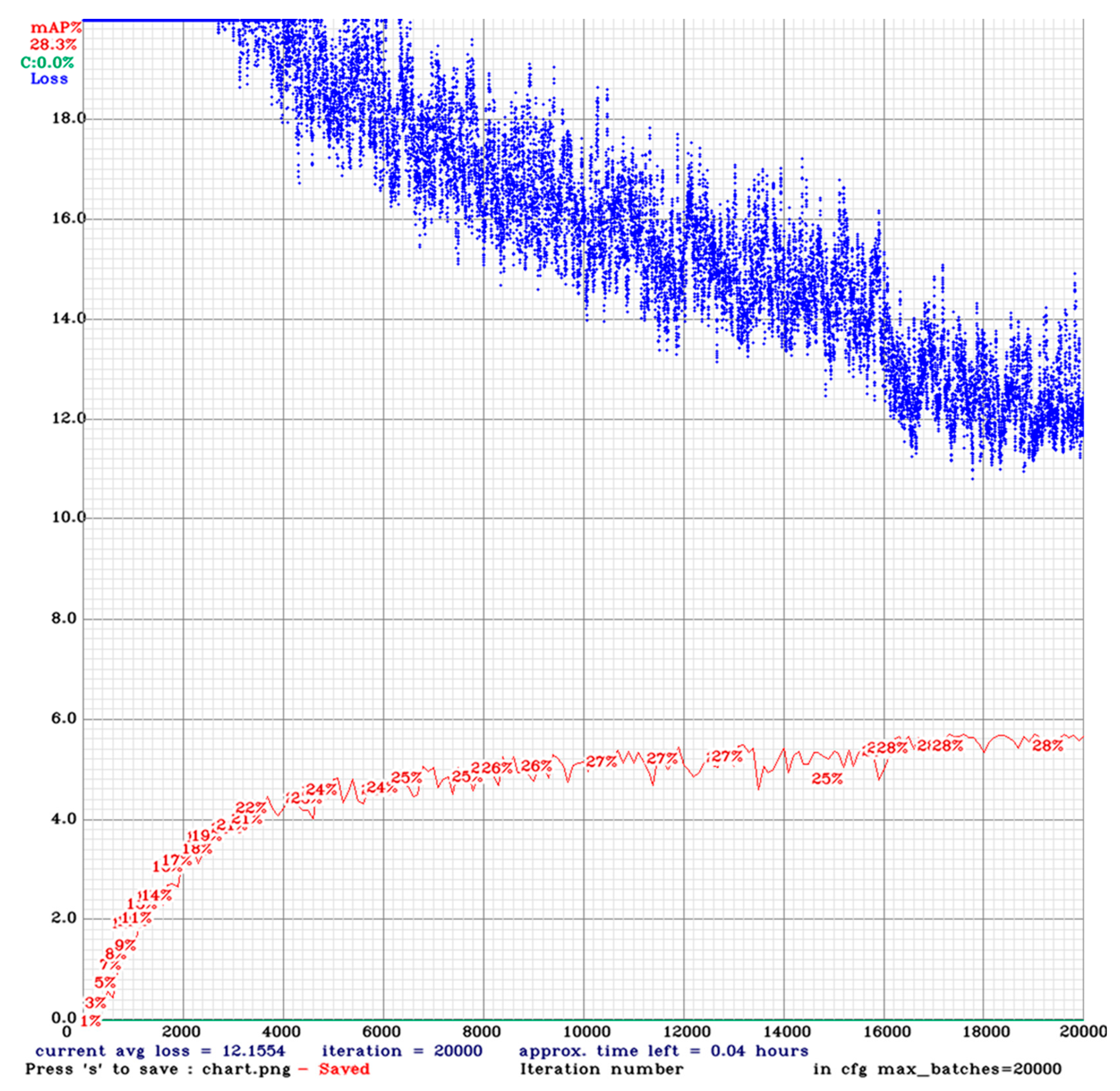
In terms of computational effort, as indicated in the introduction of this chapter, training run time varies significantly depending on the resolution of the image (see also Table 3). Figure 7 presents the progression of a training run for a 352 × 352 image resolution that requires 20,000 iterations. The red curve represents mAP, which increases as the model’s accuracy improves during training, while the blue curve corresponds to the training loss, which decreases as the model optimizes its parameters progressively. In this case, the 20,000 iterations of complete training require 378 min of computational time.
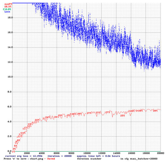
Figure 7.
Progression of mean average precision (mAP) as training iterations increase in the 352 × 352 case. The blue line represents the training loss during training iterations, while the red line shows the mAP at different training iterations.
Thus, an important aspect to consider is the time required to perform the full testing of the 48 different combinations of hyperparameters in two repetitions (a total of 40 days of computational time using the above computer system). The significant computational effort raises a practical limitation in exploring the space spanned by multiple hyperparameters. Certainly, the factorial design offers a robust understanding of how hyperparameters affect model performance. However, the significant investment in time and resources limits its applicability to situations in which rapid model creation and development are important (such as in the logistics hubs case). This highlights the need for more efficient approaches that can reduce the time required for comprehensive testing.
5. Reducing the Computational Time of Hyperparameter Space Exploration
The basic idea in reducing the computational time required for training is to predict the performance of a fully trained model much earlier in the training process. Thus, we investigated the potential of using a value of mAP that results from only a few hundred training iterations instead of the 20,000 iterations required for full model training. The metric used in this analysis is the highest validation mAP value observed between the 400th iteration and the early termination point.
We determined the iteration threshold of 400 by conducting preliminary experiments in the 0–1500 iteration range, where we observed that in early iterations (indicatively up to 200), mAP values were close to 0% due to random initialization of weights and early-stage parameter adjustments. At iteration range 0–600, max mAP reached a value a bit more than 5%, and at iteration range 0–1500, it reached a value of 14.3%. Based on these observations, we selected an iteration threshold between 200 and 600.
To identify the appropriate early training termination points, we used a two-step approach:
- We performed a correlation analysis to assess the relationship between the best validation mAP results obtained from exhaustive training vs. those obtained by early termination. This analysis was performed for each of three image size values {352 × 352, 416 × 416, 832 × 832}.
- For the promising image sizes, we ranked the best validation mAP results provided by exhaustive training from best to worst. We compared those against the maximum mAP results for the different termination points to assess possible divergence in ranking sequences.
Regarding step 1, for each of the three image resolutions, we determined the correlation between (a) the maximum validation mAP achieved for each combination of the remaining parameters (16 combinations) through exhaustive training and (b) the maximum validation mAP achieved in the training iteration ranges of 400–600, 400–1000 and 400–1500, for the same hyperparameter combinations. For example, for image resolution 832 × 832 (see Figure 8), a close correlation was observed between the best validation mAP from exhaustive training (x-axis) and the maximum validation mAP achieved in the interval between 400 and 1000 iterations (y-axis) for the 16 experiments. R2 is equal to 0.964.
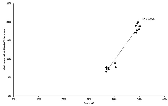
Figure 8.
Correlation between maximum validation mAP achieved through exhaustive training and maximum mAP in the interval of 400–1000 iterations for the 832 × 832 image size.
Table 5 presents the results of the entire correlation analysis. For the 352 × 352 resolution case, the correlation coefficient (R2) increases significantly with longer training durations, from 0.6722 in the 400–600 iteration case to 0.9114 in the 400–1500 iteration case. This validates the intuitive hypothesis that the mAP value produced by more extensive (but still brief) training sessions predicts the final model performance more closely. The 414 × 416 and 832 × 832 image resolution cases result in improved R2 values. Here, R2 also improves for the increased iteration cases. A notable exception is the 400–600 iteration case for the 416 × 416 resolution.
Table 5.
Correlation coefficient R2 between the values of mAP resulting from early training termination vs. those of exhaustive training performance across different image resolutions.
In the 832 × 832 resolution case, the correlation between the maximum mAP achieved during early iterations and in exhaustive training is significantly strengthened as the number of iterations increases, reaching an R2 value of 0.9714 in the range of 400–1500 iterations. This indicates that longer training periods can be highly predictive of the final model’s performance. In the case of the 400–600 iteration range, the low R2 value is due to the high volatility of the values of the model’s weights during the early stages of training.
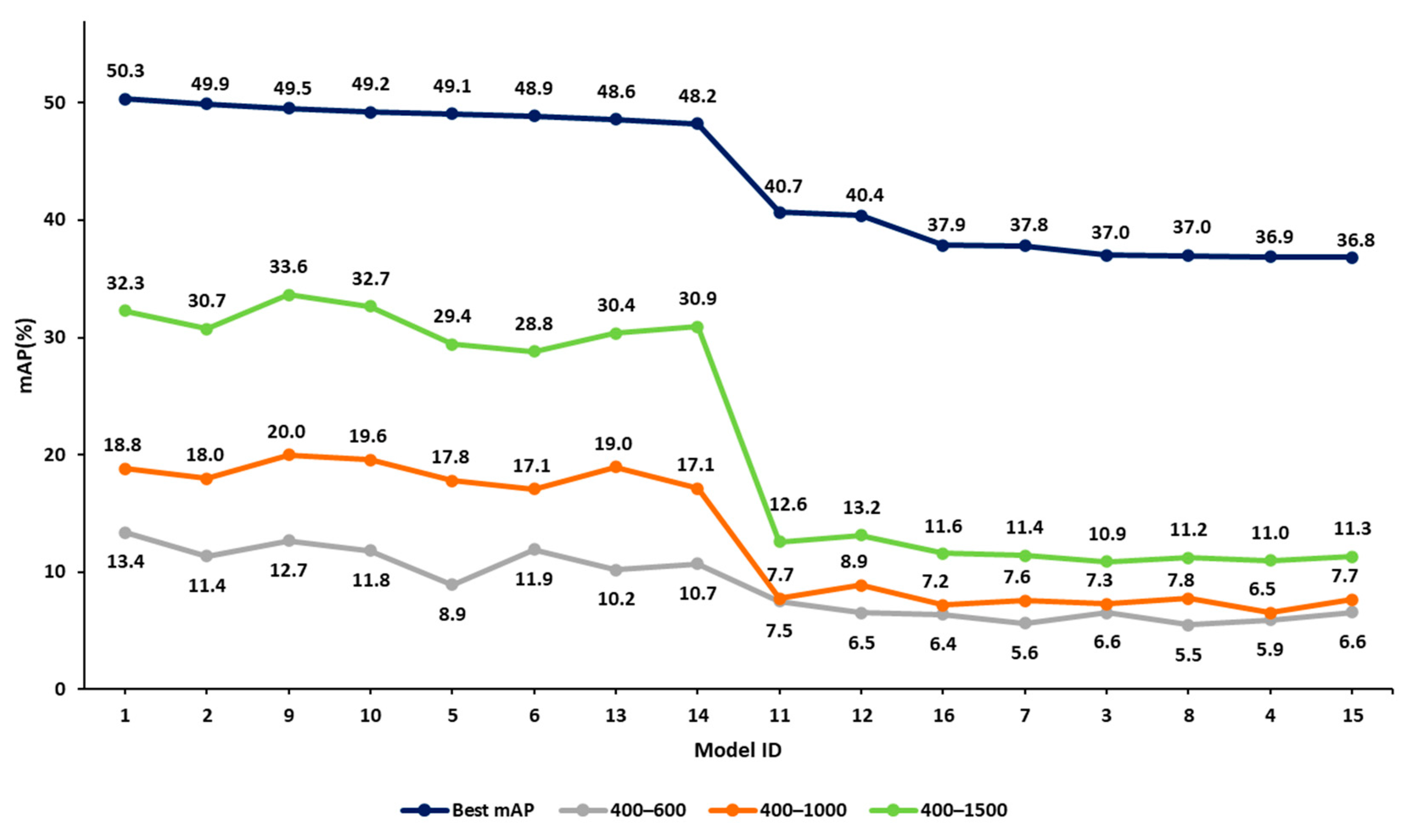
In step 2 of our approach, we listed all 16 hyperparameter combinations in decreasing order of mAP values for the 832 × 832 image resolution case. Figure 9 presents four curves of mAP related to exhaustive training and the three early termination cases. The x-axis represents the model ID (model with a different hyperparameter combination), which is sorted based on decreasing mAP values of the exhaustive training case. The other three curves follow the same experiment sequence. The y-axis represents the mAP values.

Figure 9.
Comparison of validation mAP values at various termination points against the exhaustive values obtained from training for the 832 × 832 image size. All mAP values are given in %.
Focusing on the top two curves of Figure 9, corresponding to the exhaustive training and the 400–1500 cases, it appears that early termination mAP values align well with the exhaustive training mAP values. For example, the top-performing combination of the 400–1500 case corresponds to model 9. In the exhaustive training case, the performance of this model is within 0.8% of the best combination. A similar result is obtained for the 400–1000 iteration range. However, the 400–600 iteration range does not present similar reliability. These observations indicate that knowledge of early performance can be a useful predictor of the performance of the fully trained model, provided that the iteration range is adequate (termination point 1000 iterations or more in this example).
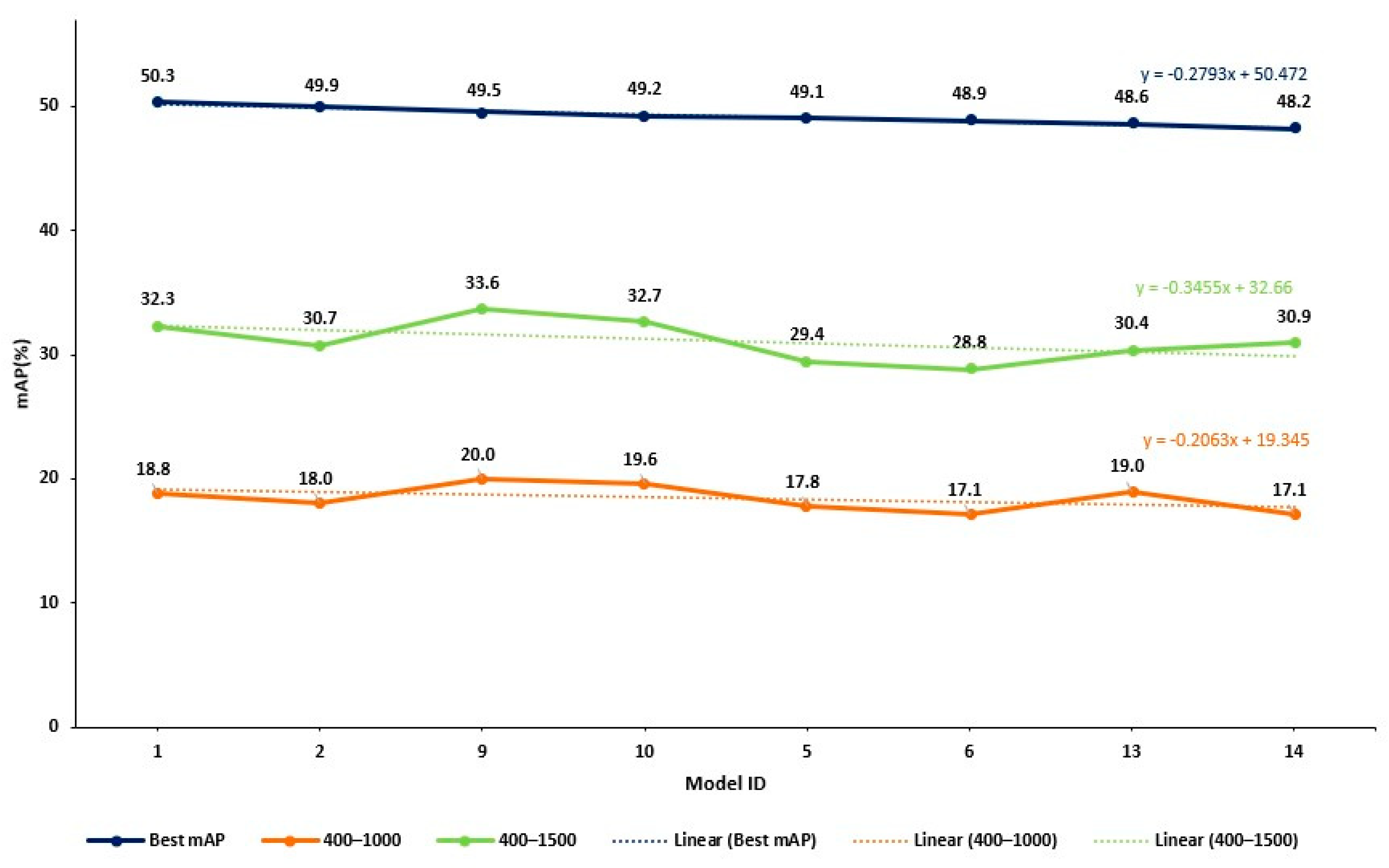
Note that the curves related to 400–1000 and 400–1500 iteration ranges present a fluctuation in the mAP value (see Figure 9). This is not unexpected, given that early termination has not allowed the final convergence of the model parameter values. However, as Figure 10 below shows, there is a declining trend in the values of the 400–1000 and 400–1500 iteration cases, quite similar to the one related to the exhaustive training case (the slopes of the three lines are presented in Figure 10 below). This is quite encouraging and seems to support our argument. In addition, the early terminated models predict the significant drop in performance observed after the model with ID 14, caused by the change in the box loss function. Specifically, models 1, 2, 9, 10, 5, 6, 13 and 14 use IoU as their box loss function, while models 11, 12, 16, 7, 3, 8, 4 and 15 use GIoU.
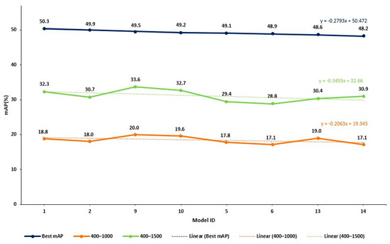
Figure 10.
Comparison of mAP trends across different training termination points.
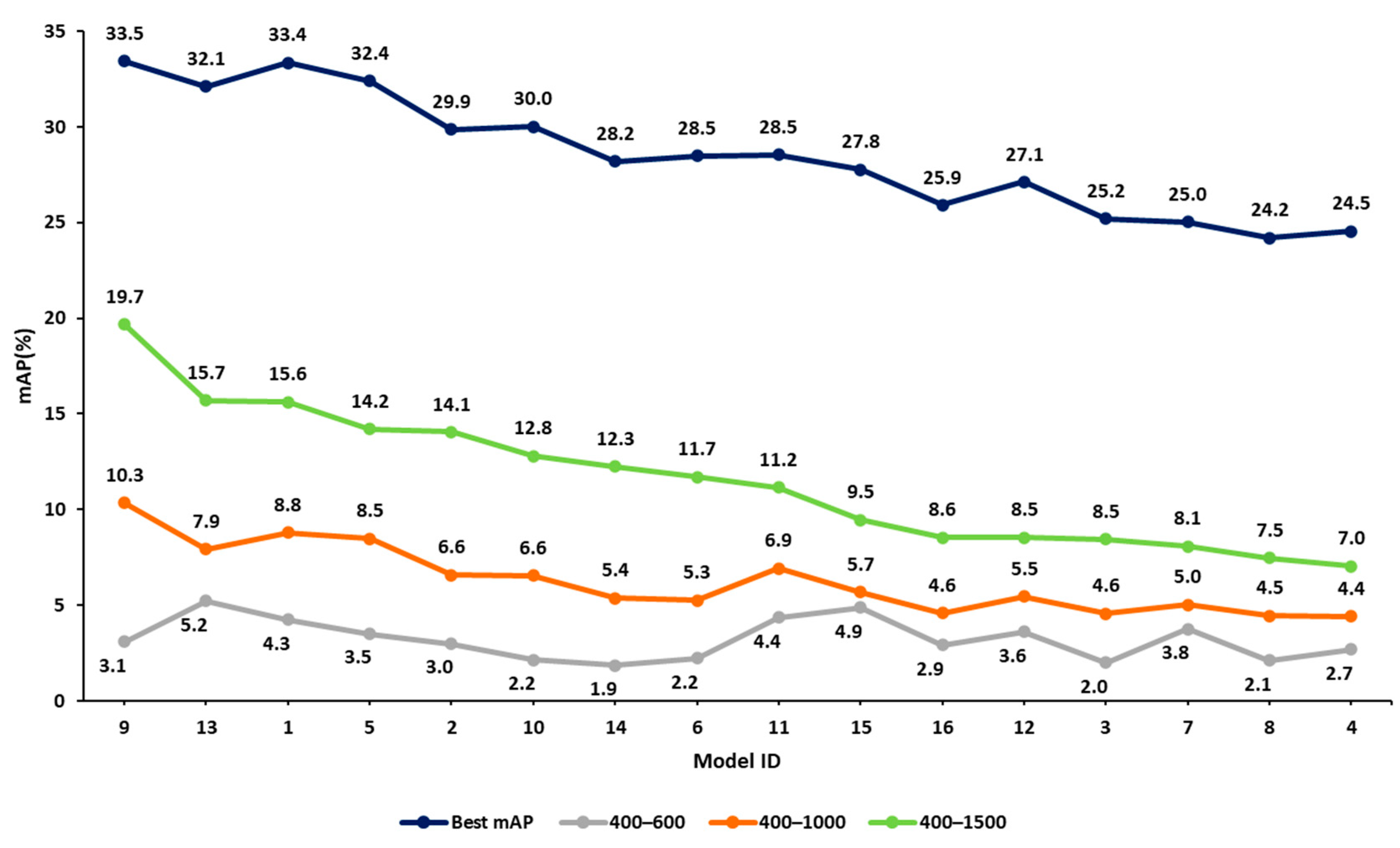
Similar results are obtained for the 416 × 416 resolution images (see Figure 11). In this case, mAP deterioration in the exhaustive training results is more gradual (no discernable step change). For both the 400–1500 and the 400–1000 early termination cases, the deterioration trend is preserved. Furthermore, the top-performing combination of exhaustive training attains the top mAP values in both early termination cases, possibly a favorable coincidence. As expected from the corresponding R2 value of Table 5, the 400–600 early termination case does not yield useful results.
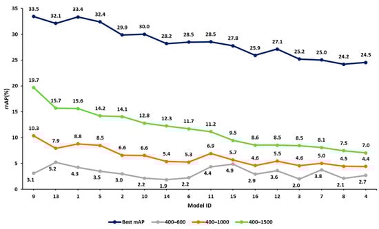
Figure 11.
Comparison of validation mAP values at various termination points against the exhaustive values obtained from training for the 416 × 416 image size. All mAP values are given in %.
For the 352 × 352 image resolutions, the distinction between high- and low-performing hyperparameter combinations in the early termination cases deteriorates further. Thus, the maximum mAP resulting from early termination of training (at least up to 1500 iterations) is not considered to be a reliable performance predictor of the fully trained model.
The analysis of the mAP curves in Figure 9, Figure 10 and Figure 11 indicates that for the 832 × 832 and the 416 × 416 image resolutions, a good predictor of model performance appears to be the maximum mAP value obtained from training sessions terminated early at 1500 or 1000 iterations. In this example case, it appears that a good trade-off between computational time and prediction ability is achieved by using image resolution 416 × 416, performing training for up to 1500 iterations and using the maximum mAP found in the range of 400 to 1500 iterations. For this case, the computational time is about 38 min, which is an order of magnitude less than the 492 min required for complete training of the model (20,000 iterations).
In step 2 of our approach (see above), for the lowest resolution (352 × 352) and shortest training duration (400–600 iterations), the models related to early termination failed to predict the performance of the fully trained models. However, at higher resolutions (416 × 416 and 832 × 832), the ability to correctly differentiate the performance under various hyperparameter combinations improves. For the 416 × 416 resolution, increasing iterations from 400–600 to 400–1500 improves success in detecting top-performing models from 20% to 80% and success in identifying the worst-performing models from 40% to 80%. At 832 × 832 resolution, the approach achieves success in detecting top-performing configurations (by 80%) across all iteration ranges. Also, the ability to identify the worst-performing configurations improves significantly with longer training—rising from 60% (400–600) to 100% (400–1500). This suggests that at higher resolutions, additional training iterations enable the model to better differentiate between all hyperparameter configurations, leading to more reliable predictions.
The above analysis indicates the following:
- The maximum mAP value obtained by early termination of the training process is a good indicator of the relative performance of the fully trained model;
- The hyperparameter combination corresponding to the highest achieved mAP in early termination of training will result in a near-optimal model when exhaustive training is completed.
6. Validation Experiments
We conducted an experimental study to validate the performance of the YOLOv3 models in port surveillance operations. For this study, we used the custom experimental set-up of Appendix A.
To assess and compare between models, we used two different datasets:
- The VisDrone Test-Development dataset (see Section 3.2);
- A specialized test dataset (DeOPSys dataset) we developed to encompass the conditions of port surveillance.
Each dataset has characteristics that help validate the YOLOv3 model’s ability to generalize across different environments and scenarios.
6.1. Validation Using the VisDrone Test Dataset
Table 6 presents the performance of the models corresponding to the 16 hyperparameter combinations when tested with the VisDrone test dataset. The models are listed in descending order of performance with respect to the early training termination case of Image resolution 416 × 416, iteration range 400–1500. The first two columns of Table 6 indicate the model ID and the mAP values obtained in early termination training (same values as in the green curve of Figure 11 but in descending order of mAP). The third column presents the mAP values obtained from these models when fully trained on the 832 × 832 image resolution and applied to the images of the VisDrone test dataset, while the fourth column presents the difference between these latter mAP values with the best mAP value obtained.
Table 6.
The performance of the 16 models ranked in decreasing mAP value of early training termination (VisDrone test dataset).
Referring to the data of Table 6, the highest achieved mAP value by a fully trained model is 38.82% and corresponds to model 5. Model 9, which had the highest mAP value during the early termination process, achieved a mAP value of 37.43%, which is only 1.38% lower than the highest mAP score. Furthermore, model 1, which displayed the highest training performance during the factorial experiments (mAP value of 50.3% in the 832 × 832 case (see Figure 8) and the third best performance in early training termination, achieved a mAP value in the VisDrone test dataset of 38.68%, that is 0.14% less than the highest value of model 5. Thus, the following conclusions could be made:
- The model corresponding to the hyperparameter combination identified as best in full training had an excellent performance in the independent VisDrone test subset;
- The model corresponding to the hyperparameter combination identified as best in early terminated training also had a very good performance in the independent VisDrone test subset.
This indicates that the factorial method using full and, most importantly, early terminated training identifies near-optimal combinations of training hyperparameters.
Four of the top five hyperparameter combinations identified by the early termination method (corresponding to models 5, 1, 2 and 13) were also ranked among the top five performing models in the 832 × 832 VisDrone test. This also supports the value of the proposed method to identify high-performance hyperparameter combinations using lower-resolution experiments with early termination training.
In order to test the applicability and lack of overfitting in datasets with other but relevant image characteristics, we performed experiments using a UAV image set that we developed in our lab (DeOPSys dataset). The performance of the best-identified model by the proposed method was consistent with the performance of the model in the VisDrone dataset and actually surpassed the latter. This provided additional and strong evidence that model training during hyperparameter tuning did not lead to dataset-specific overfitting.
6.2. Validation Using the DeOPSys Test Dataset
We employed an independent dataset generated in our lab to (a) validate the robustness of the proposed method with respect to the data (in addition to the work described in Section 4.2) and examine the applicability of the results obtained in practical situations.
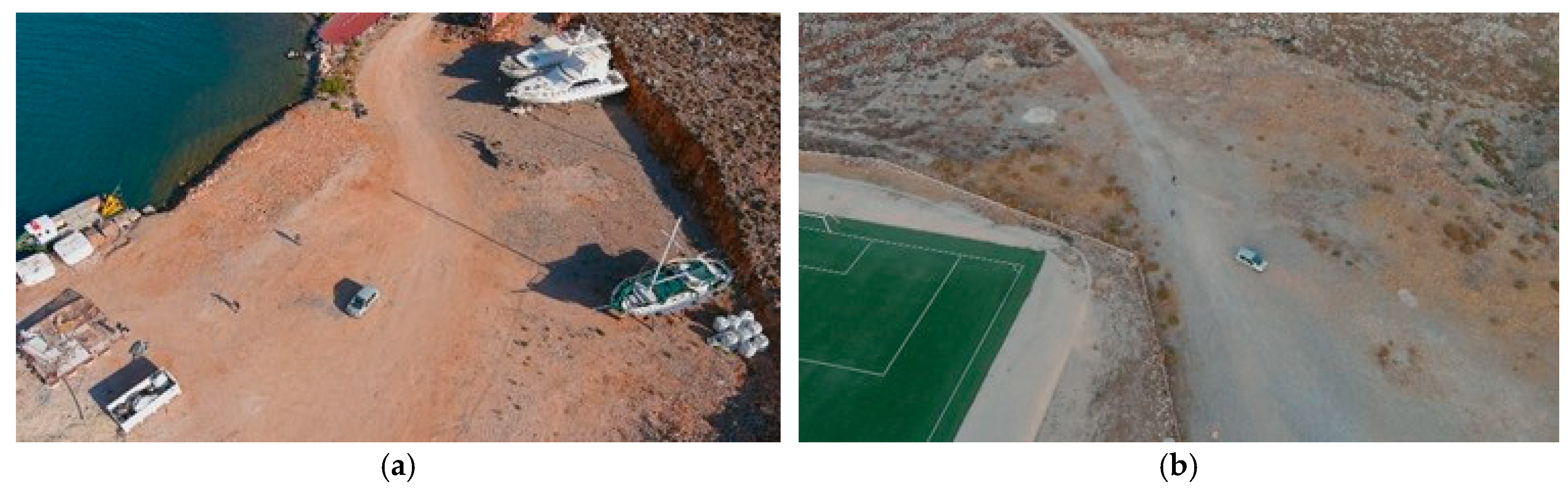
The dataset generated by our DeOPSys lab [58] consists of 722 high-resolution images taken from UAVs over two locations on the island of Chios, Greece: (a) Tholos port/shipyard (Figure 12a) and (Figure 12b) a rural area in the northern part of the island (Figure 12b). The images were captured under varying light conditions (daylight and dusk) and from different altitudes (15 m, 30 m and 50 m) [59]. They were annotated using LabelImg 1.8.6 [60] to identify and mark objects, such as persons and cars, resulting in a total of 1218 annotated objects.

Figure 12.
(a) Port in the area of Tholos in daylight at an altitude of 50 m; (b) area without settlements in Lagada in low light conditions at an altitude of 50 m.
The analysis applied to the VisDrone Test-Development dataset was also applied to the DeOPSys dataset. Table 7, structured similarly to Table 6, presents the performance results of the 16 models in descending order of performance for early termination.
Table 7.
The performance of the 16 models ranked in decreasing mAP resulting from early termination of training (DeOPSys test dataset).
Table 7.
The performance of the 16 models ranked in decreasing mAP resulting from early termination of training (DeOPSys test dataset).
| Early Termination Strategy | Fully Trained Models at 832 × 832 | ||
|---|---|---|---|
| Model ID | Validation mAP (Early Termination) | Test mAP | Difference with Best mAP |
| 9 | 19.7% | 73.36% | 1.58% |
| 13 | 15.7% | 72.40% | 2.54% |
| 1 | 15.6% | 73.87% | 1.07% |
| 5 | 14.2% | 74.94% | - |
| 2 | 14.1% | 74.66% | 0.28% |
| 10 | 12.8% | 74.72% | 0.22% |
| 14 | 12.3% | 71.25% | 3.69% |
| 6 | 11.7% | 74.44% | 0.50% |
| 11 | 11.2% | 72.12% | 2.82% |
| 15 | 9.5% | 67.13% | 7.81% |
| 16 | 8.6% | 69.07% | 5.87% |
| 12 | 8.5% | 74.19% | 0.75% |
| 3 | 8.5% | 66.94% | 8.00% |
| 7 | 8.1% | 73.12% | 1.82% |
| 8 | 7.5% | 67.55% | 7.39% |
| 4 | 7.0% | 70.27% | 4.67% |
The highest test mAP achieved by a fully trained model (model 5) was 74.94% (a particularly high value). Model 1, which displayed the best performance in the factorial experiments, achieved a test mAP of 73.87%, which is only 1.07% lower than model 5. Similarly, the model achieved the best performance in early termination training (model 9) and achieved a test mAP of 73.36%, a difference of 1.58% from the performance of model 5 and 0.51% from the performance of model 1.
These test results indicate the following:
- Superior performance is obtained by the top models of the factorial experiments, as well as the top models of the early termination approach. In fact, the performance in the independent DeOPSys dataset was significantly better than the one corresponding to the VisDrone dataset used in the original model training.
- In this case, the early termination approach was also able to identify the high-performing hyperparameter combinations.
- The proposed method is robust across datasets and may identify hyperparameter combinations resulting in high-performing models.
- Model training during hyperparameter tuning did not lead to dataset-specific overfitting.
7. Conclusions and Discussion
7.1. Hyperparameter Tuning and Early Termination Strategy
In this study, we focused on optimizing the training process of the YOLOv3 algorithm for drone surveillance. This involved two aspects: (a) tuning of key training hyperparameters through exploration of the hyperparameter space and (b) use of an early termination strategy to rationalize the long computational times involved.
Factorial experiments demonstrated the importance of hyperparameter selection on model performance. During training/validation, the best-performing model achieved a mAP value of 50.33%, while the worst-performing model achieved a mAP value of 36.8%, a considerable difference in performance. Factors such as image resolution, box loss functions and anchor sizes were found to have the most significant effect on mAP. Furthermore, ANOVA may systematically explore the effects of all hyperparameters and all their interactions on model performance.
However, the scalability of factorial design is limited as the number of hyperparameters increases. In our case, the factorial design required approximately 40 days of computational time in the (weak) system we used, highlighting the need for more efficient tuning methods.
To address this challenge, an early termination strategy was introduced, which reduced processing time by up to 92%. Despite the reduced computational cost, the methodology still identified high-performing hyperparameter combinations. The largest observed mAP difference between the best-performing model trained exhaustively and the best-performing model identified during the early termination process (and then trained exhaustively) was only 0.8%. Under this limited mAP difference, the best-performing model identified through early termination remains effective in the object’s detection case under study, ensuring that it can still identify potential threats or targets in logistics surveillance. In practical applications, this limited accuracy trade-off is acceptable, given the significant reduction in computational cost, making the approach well-suited for real-time drone-based surveillance. It is also noted that the proposed early termination approach is highly scalable.
Testing of the best-performing model using a specially developed dataset that meets the characteristics of logistics hubs further supported the effectiveness of the proposed method; that is, factorial exploration of the hyperparameter space with early training termination may be used to develop highly performing models.
7.2. Future Research Directions and Potential of Advanced Methods
Further research may explore other training hyperparameters related to structural changes in neural network architecture. Additionally, integrating more intelligent search methods, such as Bayesian optimization, genetic algorithms or reinforcement learning, could enhance the efficiency of hyperparameter tuning.
These techniques may provide the potential to study a greater number of hyperparameters (beyond the five ones investigated in the current study), addressing the scalability limitation of factorial designs. Exploring a wider hyperparameter space intelligently (as opposed to the brute force approach of the current study) may provide the opportunity to reveal configurations that can achieve higher accuracy and detection efficiency with reasonable computational cost.
From our experience in ongoing work beyond the scope of this manuscript, we have observed that genetic algorithms (GA) significantly reduce computational costs compared to a full factorial approach. Specifically, in an experiment tuning 16 hyperparameters instead of the 5 used in this study, a full factorial design would require 65,536 models. However, by applying a GA with a population size of 30, 20 generations and five parents, the algorithm converges by running a bit more than 500 models, significantly reducing computational requirements. This highlights the potential of GA as an efficient alternative to exhaustive hyperparameter tuning methods. However, it should be noted that genetic algorithms are limited in identifying the effects of hyperparameters and their interactions on model performance.
Author Contributions
Conceptualization, G.T., K.M. and I.M.; methodology, G.T. and I.M.; software, G.T.; supervision, I.M. and K.M. All authors have read and agreed to the published version of the manuscript.
Funding
This research was funded by the Intelligent Research Infrastructure for Shipping, Supply Chain, Transport and Logistics (ENIRISST+) project (MIS 5027930) from the NSRF 2014-2020 Operational Programme “Competitiveness, Entrepreneurship, Innovation”.
Data Availability Statement
Data included in the article or references.
Conflicts of Interest
The authors declare no conflicts of interest.
Appendix A
The Experimental Set-Up
The experimental set-up is presented in Figure A1. The UAV system is equipped with a smart controller and a display/navigation interface that provides real-time video feedback and navigation data. The display/navigation system is connected to a wireless network. A laptop computer connected to the same network receives the image and displays it on the computer screen. Each frame of the desktop is recorded using a screen recording software built with Python version 3.10 and based on win32gui, win32ui and win32con libraries. The computer preprocesses each image, cropping and resizing it as guided by another Python script that uses specialized image processing routines provided by OpenCV. The preprocessed screenshots are then passed as input to the YOLO detector via an OpenCV dnn module. The detection results are recorded and stored on the computer storage module, part of which is the input video, showing the bounding boxes, classes and class probabilities for each detected object.
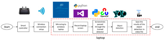
Figure A1.
Integrated object recognition system via screen mirroring.
Figure A1.
Integrated object recognition system via screen mirroring.

References
- Cempírek, V.; Nachtigall, P.; Široký, J. Security in Logistics. Open Eng. 2016, 6, 634–641. [Google Scholar] [CrossRef]
- SOLAS XI-2 and the ISPS Code. Available online: https://www.imo.org/en/OurWork/Security/Pages/SOLAS-XI-2%20ISPS%20Code.aspx (accessed on 22 May 2024).
- Standards. Available online: https://tapaemea.org/standards-trainings/ (accessed on 22 May 2024).
- Dias, E.; Fontana, C.; Mori, F.H.; Facioli, L.P.; Zancul, P.J. Security Supply Chain. In Proceedings of the 12th WSEAS International Conference on SYSTEMS, Heraklion, Greece, 22–24 July 2008. [Google Scholar]
- Enirisst Plus. Available online: https://enirisst-plus.gr/ (accessed on 12 January 2024).
- Inagaki, T.; Stahre, J. Human Supervision and Control in Engineering and Music: Similarities, Dissimilarities, and Their Implications. Proc. IEEE 2004, 92, 589–600. [Google Scholar] [CrossRef]
- IFSEC Insider. Role of CCTV Cameras: Public, Privacy and Protection. In Security and Fire News and Resources; IFSEC Insider: London, UK, 2021. [Google Scholar]
- Xie, J.; Zheng, Y.; Du, R.; Xiong, W.; Cao, Y.; Ma, Z.; Cao, D.; Guo, J. Deep Learning-Based Computer Vision for Surveillance in ITS: Evaluation of State-of-the-Art Methods. IEEE Trans. Veh. Technol. 2021, 70, 3027–3042. [Google Scholar] [CrossRef]
- Hossain, S.; Lee, D.J. Deep Learning-Based Real-Time Multiple-Object Detection and Tracking from Aerial Imagery via a Flying Robot with GPU-Based Embedded Devices. Sensors 2019, 19, 3371. [Google Scholar] [CrossRef] [PubMed]
- Unlu, E.; Zenou, E.; Riviere, N.; Dupouy, P.-E.; Zenou, E.; Riviere, N.; Dupouy, P.-E. An Autonomous Drone Surveillance and Tracking Architecture. Electron. Imaging 2019, 31, 1–7. [Google Scholar] [CrossRef]
- Won, J.-H.; Lee, D.-H.; Lee, K.-M.; Lin, C.-H. An Improved YOLOv3-Based Neural Network for De-Identification Technology. In Proceedings of the 2019 34th International Technical Conference on Circuits/Systems, Computers and Communications (ITC-CSCC), JeJu, Republic of Korea, 23–26 June 2019; pp. 1–2. [Google Scholar]
- Wei Xun, D.T.; Lim, Y.L.; Srigrarom, S. Drone Detection Using YOLOv3 with Transfer Learning on NVIDIA Jetson TX2. In Proceedings of the 2021 Second International Symposium on Instrumentation, Control, Artificial Intelligence, and Robotics (ICA-SYMP), Bangkok, Thailand, 20 January 2021; pp. 1–6. [Google Scholar]
- Shao, J.; Chen, S.; Li, Y.; Wang, K.; Yin, Z.; He, Y.; Teng, J.; Sun, Q.; Gao, M.; Liu, J.; et al. INTERN: A New Learning Paradigm Towards General Vision. arXiv 2021, arXiv:2111.08687v2. [Google Scholar]
- Lyu, L.; Yu, H.; Ma, X.; Chen, C.; Sun, L.; Zhao, J.; Yang, Q.; Yu, P.S. Privacy and Robustness in Federated Learning: Attacks and Defenses. IEEE Trans. Neural Netw. Learn. Syst. 2022, 35, 8726–8746. [Google Scholar] [CrossRef] [PubMed]
- Walambe, R.; Marathe, A.; Kotecha, K. Multiscale Object Detection from Drone Imagery Using Ensemble Transfer Learning. Drones 2021, 5, 66. [Google Scholar] [CrossRef]
- Mishra, B.; Garg, D.; Narang, P.; Mishra, V. Drone-Surveillance for Search and Rescue in Natural Disaster. Comput. Commun. 2020, 156, 1–10. [Google Scholar] [CrossRef]
- Singh, A.; Patil, D.; Omkar, S.N. Eye in the Sky: Real-Time Drone Surveillance System (DSS) for Violent Individuals Identification Using ScatterNet Hybrid Deep Learning Network. In Proceedings of the 2018 IEEE/CVF Conference on Computer Vision and Pattern Recognition Workshops (CVPRW), Salt Lake City, UT, USA, 18–22 June 2018; pp. 1710–17108. [Google Scholar]
- Lin, T.-Y.; Dollár, P.; Girshick, R.; He, K.; Hariharan, B.; Belongie, S. Feature Pyramid Networks for Object Detection. In Proceedings of the 2017 IEEE Conference on Computer Vision and Pattern Recognition (CVPR), Honolulu, HI, USA, 21–26 July 2017; pp. 936–944. [Google Scholar]
- Cui, F.; Zou, L.; Song, B. Edge Feature Extraction Based on Digital Image Processing Techniques. In Proceedings of the 2008 IEEE International Conference on Automation and Logistics, Qingdao, China, 1–3 September 2008; pp. 2320–2324. [Google Scholar]
- Sahin, O.; Ozer, S. YOLODrone: Improved YOLO Architecture for Object Detection in Drone Images. In Proceedings of the 2021 44th International Conference on Telecommunications and Signal Processing (TSP), Brno, Czech Republic, 26 July 2021; pp. 361–365. [Google Scholar]
- Jadhav, R.; Patil, R.; Diwan, A.; Rathod, S.M.; Sharma, A. Drone Based Object Detection Using AI. In Proceedings of the 2022 International Conference on Signal and Information Processing (IConSIP), Pune, India, 25–27 August 2022; pp. 1–5. [Google Scholar]
- Tan, L.; Lv, X.; Lian, X.; Wang, G. YOLOv4_Drone: UAV Image Target Detection Based on an Improved YOLOv4 Algorithm. Comput. Electr. Eng. 2021, 93, 107261. [Google Scholar] [CrossRef]
- Kyrkou, C.; Plastiras, G.; Theocharides, T.; Venieris, S.I.; Bouganis, C.-S. DroNet: Efficient Convolutional Neural Network Detector for Real-Time UAV Applications. In Proceedings of the 2018 Design, Automation & Test in Europe Conference & Exhibition (DATE), Dresden, Germany, 9–23 March 2018; pp. 967–972. [Google Scholar]
- Benhadhria, S.; Mansouri, M.; Benkhlifa, A.; Gharbi, I.; Jlili, N. VAGADRONE: Intelligent and Fully Automatic Drone Based on Raspberry Pi and Android. Appl. Sci. 2021, 11, 3153. [Google Scholar] [CrossRef]
- Ashraf, S.; Ahmed, T. Sagacious Intrusion Detection Strategy in Sensor Network. In Proceedings of the 2020 International Conference on UK-China Emerging Technologies (UCET), Glasgow, UK, 20–21 August 2020; pp. 1–4. [Google Scholar]
- Lee, Y.Y.; Abdul Halim, Z.; Ab Wahab, M.N. License Plate Detection Using Convolutional Neural Network–Back to the Basic With Design of Experiments. IEEE Access 2022, 10, 22577–22585. [Google Scholar] [CrossRef]
- Chen, S.-H.; Jang, J.-H.; Youh, M.-J.; Chou, Y.-T.; Kang, C.-H.; Wu, C.-Y.; Chen, C.-M.; Lin, J.-S.; Lin, J.-K.; Liu, K.F.-R. Real-Time Video Smoke Detection Based on Deep Domain Adaptation for Injection Molding Machines. Mathematics 2023, 11, 3728. [Google Scholar] [CrossRef]
- Mantau, A.J.; Widayat, I.W.; Adhitya, Y.; Prakosa, S.W.; Leu, J.-S.; Köppen, M. A GA-Based Learning Strategy Applied to YOLOv5 for Human Object Detection in UAV Surveillance System. In Proceedings of the 2022 IEEE 17th International Conference on Control & Automation (ICCA), Naples, Italy, 27–30 June 2022; pp. 9–14. [Google Scholar]
- Hou, C.; Guan, Z.; Guo, Z.; Zhou, S.; Lin, M. An Improved YOLOv5s-Based Scheme for Target Detection in a Complex Underwater Environment. J. Mar. Sci. Eng. 2023, 11, 1041. [Google Scholar] [CrossRef]
- Redmon, J.; Farhadi, A. YOLOv3: An Incremental Improvement. arXiv 2018, arXiv:1804.02767. [Google Scholar] [CrossRef]
- Ma, H.; Liu, Y.; Ren, Y.; Yu, J. Detection of Collapsed Buildings in Post-Earthquake Remote Sensing Images Based on the Improved YOLOv3. Remote Sens. 2020, 12, 44. [Google Scholar] [CrossRef]
- Huang, C.-Y.; Lin, I.-C.; Liu, Y.-L. Applying Deep Learning to Construct a Defect Detection System for Ceramic Substrates. Appl. Sci. 2022, 12, 2269. [Google Scholar] [CrossRef]
- Tepteris, G.; Mamasis, K.; Minis, I. State of the Art Object Detection and Recognition Methods (Draft) | DeOPSys Lab. Available online: https://deopsys.aegean.gr/node/280 (accessed on 21 August 2024).
- Zhu, P.; Wen, L.; Du, D.; Bian, X.; Fan, H.; Hu, Q.; Ling, H. Detection and Tracking Meet Drones Challenge. IEEE Trans. Pattern Anal. Mach. Intell. 2022, 44, 7380–7399. [Google Scholar] [CrossRef]
- Wu, K.; Bai, C.; Wang, D.; Liu, Z.; Huang, T.; Zheng, H. Improved Object Detection Algorithm of YOLOv3 Remote Sensing Image. IEEE Access 2021, 9, 113889–113900. [Google Scholar] [CrossRef]
- Igiri, C.; Uzoma, A.; Silas, A. Effect of Learning Rate on Artificial Neural Network in Machine Learning. Int. J. Eng. Res. 2021, 4, 359–363. [Google Scholar]
- Batch Size in Neural Network. Available online: https://www.geeksforgeeks.org/batch-size-in-neural-network/ (accessed on 4 February 2025).
- Qingyun, F.; Lin, Z.; Zhaokui, W. An Efficient Feature Pyramid Network for Object Detection in Remote Sensing Imagery. IEEE Access 2020, 8, 93058–93068. [Google Scholar] [CrossRef]
- Yao, S.; Chen, Y.; Tian, X.; Jiang, R.; Ma, S. An Improved Algorithm for Detecting Pneumonia Based on YOLOv3. Appl. Sci. 2020, 10, 1818. [Google Scholar] [CrossRef]
- Yang, Z.; Xu, W.; Wang, Z.; He, X.; Yang, F.; Yin, Z. Combining Yolov3-Tiny Model with Dropblock for Tiny-Face Detection. In Proceedings of the 2019 IEEE 19th International Conference on Communication Technology (ICCT), Xi’an, China, 16–19 October 2019; pp. 1673–1677. [Google Scholar]
- Ortiz Castelló, V.; Salvador Igual, I.; del Tejo Catalá, O.; Perez-Cortes, J.-C. High-Profile VRU Detection on Resource-Constrained Hardware Using YOLOv3/v4 on BDD100K. J. Imaging 2020, 6, 142. [Google Scholar] [CrossRef]
- Goodfellow, I.; Bengio, Y.; Courville, A. Deep Learning; Adaptive Computation and Machine Learning; The MIT Press: Cambridge, MA, USA, 2016; ISBN 978-0-262-03561-3. [Google Scholar]
- Song, H. Multi-Scale Safety Helmet Detection Based on RSSE-YOLOv3. Sensors 2022, 22, 6061. [Google Scholar] [CrossRef] [PubMed]
- Wang, Q.; Bi, S.; Sun, M.; Wang, Y.; Wang, D.; Yang, S. Deep Learning Approach to Peripheral Leukocyte Recognition. PLoS ONE 2019, 14, e0218808. [Google Scholar] [CrossRef] [PubMed]
- Zhang, X.; Zhu, X. An Efficient and Scene-Adaptive Algorithm for Vehicle Detection in Aerial Images Using an Improved YOLOv3 Framework. ISPRS Int. J. Geo-Inf. 2019, 8, 483. [Google Scholar] [CrossRef]
- Cui, W.; Zhang, W.; Green, J.; Zhang, X.; Yao, X. YOLOv3-Darknet with Adaptive Clustering Anchor Box for Garbage Detection in Intelligent Sanitation. In Proceedings of the 2019 3rd International Conference on Electronic Information Technology and Computer Engineering (EITCE), Xiamen, China, 16–19 October 2019; pp. 220–225. [Google Scholar]
- Rezatofighi, H.; Tsoi, N.; Gwak, J.; Sadeghian, A.; Reid, I.; Savarese, S. Generalized Intersection Over Union: A Metric and a Loss for Bounding Box Regression. In Proceedings of the 2019 IEEE/CVF Conference on Computer Vision and Pattern Recognition (CVPR), Long Beach, CA, USA, 15–20 June 2019; pp. 658–666. [Google Scholar]
- Zhang, B.; Wang, G.; Wang, H.; Xu, C.; Li, Y.; Xu, L. Detecting Small Chinese Traffic Signs via Improved YOLOv3 Method. Math. Probl. Eng. 2021, 2021, 1–10. [Google Scholar] [CrossRef]
- Vilcapoma, P.; Parra Meléndez, D.; Fernández, A.; Vásconez, I.N.; Hillmann, N.C.; Gatica, G.; Vásconez, J.P. Comparison of Faster R-CNN, YOLO, and SSD for Third Molar Angle Detection in Dental Panoramic X-Rays. Sensors 2024, 24, 6053. [Google Scholar] [CrossRef]
- Muthuraja, M.; Arriaga, O.; Plöger, P.; Kirchner, F.; Valdenegro-Toro, M. Black-Box Optimization of Object Detector Scales. arXiv 2020, arXiv:2010.15823. [Google Scholar]
- Kee, E.; Chong, J.J.; Choong, Z.J.; Lau, M. Object Detection with Hyperparameter and Image Enhancement Optimisation for a Smart and Lean Pick-and-Place Solution. Signals 2024, 5, 87–104. [Google Scholar] [CrossRef]
- Yu, F. YOLO, Faster R-CNN, and SSD for Cloud Detection. ACE 2024, 37, 239–247. [Google Scholar] [CrossRef]
- Lv, N.; Xiao, J.; Qiao, Y. Object Detection Algorithm for Surface Defects Based on a Novel YOLOv3 Model. Processes 2022, 10, 701. [Google Scholar] [CrossRef]
- Cui, Y.; Lu, S.; Liu, S. Real-Time Detection of Wood Defects Based on SPP-Improved YOLO Algorithm. Multimed. Tools Appl. 2023, 82, 21031–21044. [Google Scholar] [CrossRef]
- Zhang, S.; Chai, L.; Jin, L. Vehicle Detection in UAV Aerial Images Based on Improved YOLOv3. In Proceedings of the 2020 IEEE International Conference on Networking, Sensing and Control (ICNSC), Nanjing, China, 30 October–2 November 2020; pp. 1–6. [Google Scholar]
- Shaotong, P.; Dewang, L.; Ziru, M.; Yunpeng, L.; Yonglin, L. Location and Identification of Insulator and Bushing Based on YOLOv3-Spp Algorithm. In Proceedings of the 2021 IEEE International Conference on Electrical Engineering and Mechatronics Technology (ICEEMT), Qingdao, China, 2–4 July 2021; pp. 791–794. [Google Scholar]
- Padilla, R.; Passos, W.L.; Dias, T.L.B.; Netto, S.L.; da Silva, E.A.B. A Comparative Analysis of Object Detection Metrics with a Companion Open-Source Toolkit. Electronics 2021, 10, 279. [Google Scholar] [CrossRef]
- DeOPSys Lab. Available online: https://deopsys.aegean.gr/ (accessed on 30 May 2024).
- Dataset—DeOPSys Dataset—DKAN Demo. Available online: https://open-data.enirisstplus.uop.gr/dataset/d8d4163e-fac6-4369-87b8-c795d76fc274 (accessed on 31 May 2024).
- Boesch, G. LabelImg for Image Annotation. Available online: https://viso.ai/computer-vision/labelimg-for-image-annotation/ (accessed on 30 May 2024).


Disclaimer/Publisher’s Note: The statements, opinions and data contained in all publications are solely those of the individual author(s) and contributor(s) and not of MDPI and/or the editor(s). MDPI and/or the editor(s) disclaim responsibility for any injury to people or property resulting from any ideas, methods, instructions or products referred to in the content. |
© 2025 by the authors. Licensee MDPI, Basel, Switzerland. This article is an open access article distributed under the terms and conditions of the Creative Commons Attribution (CC BY) license (https://creativecommons.org/licenses/by/4.0/).