Article

The Rating Scale Paradox: An Application to the Solvency 2 Framework

by
Jacopo Giacomelli
1,2,†
1
SACE S.p.A, Piazza Poli 42, 00187 Rome, Italy
2
Department of Statistics, Sapienza University of Rome, Viale Regina Elena 295, 00161 Rome, Italy
The views and opinions expressed in this article are those of the author and do not necessarily reflect the official policy or position of SACE S.p.A.
Standards 2023, 3(4), 356-372; https://doi.org/10.3390/standards3040025
Submission received: 14 June 2023 / Revised: 5 October 2023 / Accepted: 10 October 2023 / Published: 12 October 2023

Abstract

:
This work aims to identify the optimal rating scale for the rating system used by a credit insurance company subjected to the Solvency 2 regulatory framework. To do so, we apply and further develop a previously published result concerning the rating scale properties. The partition underlying a given rating scale must satisfy two needs of the rating model user: efficient information synthesis and stable semantics. Those needs cannot be addressed together in general. Nonetheless, it is possible to specify the partition as a linear combination of the two choices that meet one requirement each. We numerically show that, in general, the optimal combination is nontrivial under realistic assumptions and is mainly driven by the target return fixed by the company’s stakeholders and the debtors’ probability of default distribution.

1. Introduction

Nowadays, rating systems are widely applied across the most diverse contexts. Without claim for completeness, relevant applications include the healthcare sector [1,2,3], zero-sum games [4,5,6], psychometrics [7,8,9,10], and agronomy [11]. However, the possibly most widespread application of rating systems is the creditworthiness measurement, both in banks [12] and insurance companies [13].
In its most general sense, a rating system is a set of rules to classify a subject into a given rating class, or notch, based on processing a standardized data set associated with the subject at the evaluation time. Typically, notches constitute an ordered set known as “rating scale” or “master scale” [14,15,16,17].
The rating scale has two primary purposes, which remain the same in all the possible applications. First, the rating scale provides the user with easily understandable information. For example, in the credit risk context, the output returned by a rating system to a given counterparty provides risk underwriters and investors with immediate knowledge of the counterparty’s creditworthiness, given their awareness of the rating scale semantics. Second, the rating scale enables the construction of automated decisional systems, as each notch can activate a specific set of rules and actions regarding the evaluated subject.
In [18], we have shown that these two purposes may somewhat contrast each other. Indeed, stable semantics can lead to an inefficient decisional system. e.g., given a portfolio of risky credit debtors, a bank or other financial entity defines and calibrates an internal rating system, fixing a probability of default (PD) level associated with each notch of the rating scale (i.e., the rating scale is a priori defined through a semantics-based criterion). Without any semantics update, as the average portfolio creditworthiness improves or worsens over time, an increasing fraction of the debtors is progressively concentrated at the extreme notches of the master scale, implying that the same action (rejecting the credit request or granting the maximum credit limit) follows for each evaluated subject. In such a case, the rating model becomes useless as its discriminant power approaches zero. On the other hand, when the rating scale’s semantics is redefined too strongly, the rating model’s user loses the ability to understand the creditworthiness of the evaluated subject based on the notch that is assigned by the rating system. This kind of situation may happen if the master scale is defined and updated aiming to maximize the model efficiency in processing the available information (i.e., an information-based criterion is applied to calibrate the rating scale), implying that the same notch assumes different meanings depending on the average creditworthiness of the evaluated portfolio at different times.
Fixing a credit limit level per notch has economic consequences for a bank that applies a “rating-plus-automated-decisions” system. An automated decisional system typically aims to establish a maximum acceptable amount of exposure to the counterparty risk of each debtor. As shown in [18], a semantics-based rating scale implies a more prudential behavior of the system as the average creditworthiness of the bank’s debtors worsens over time. Conversely, an information-based rating scale implies a more efficient but less prudential attitude of the system regarding the accepted exposures.
It is neither possible nor correct to consider one of these two approaches as the best under every circumstance. The possibility to mix information-based and semantics-based criteria allows us to identify a balanced solution that best fits a specific economic operator, given its regulatory constraints and level of risk appetite.
The concept of a hybrid rating scale, discussed in [18] and this work, is new, although problems concerning the stability of rating systems and PDs have been extensively investigated in the banking literature. The most notorious and debated concept is choosing the PDs’ calibration as through-the-cycle (TTC) or point-in-time (PIT) [19,20]. Namely, TTC PDs are measured considering a risky firm’s creditworthiness fluctuations across a whole economic cycle. Conversely, PIT PDs take into account the current economic context and how a firm relates to it at the moment of its PDs’ measurement.
Indeed, the choice between PIT and TTC PDs improves a rating system’s reactivity or stability, respectively [21]. Nonetheless, this parameterization choice does not directly impact the rating scale’s semantics, which can be modified even if TTC PDs are used. In fact, the model user can redefine the score or creditworthiness range associated with each notch, regardless of the selected PDs’ calibration technique, resulting in an evolving PD per notch. On the other hand, in case PIT PDs are chosen, the model’s user can adjust the score range per notch for each PD update so that the PD associated with each notch remains always the same.
To the best of our knowledge, the problem discussed in literature most similar to the one addressed in this work is the stability-accuracy tradeoff analyzed by Cantor and Mann [22]: namely, how to choose an intermediate solution between a reactive rating system, whose frequent rating changes enable a high model’s accuracy, and a stable rating system, whose rare rating changes imply a less dynamic model, although less predictive as well. However, their approach considers the amplitude of a firm’s creditworthiness variation and the persistence of the newly measured creditworthiness level as critical elements for deciding whether to change its rating. In their study, the semantics of the model is fixed by construction. Conversely, we consider the possibility of redefining the rating scale (i.e., the model’s semantics) through time as the primary degree of freedom to be investigated, while our rating system is assumed to react instantaneously and automatically to every creditworthiness variation measured. Further, their study is limited to reducing the governance costs of managing a corporate bonds portfolio, implying a relatively low dynamic context, compared with most of the examples proposed above and especially the case of a credit insurer managing a portfolio of SMEs, which is the application investigated in the following.
This work investigates the possibility and the utility of applying the concept of hybrid master scale to the risk appetite framework of a credit insurance company [23,24,25,26,27,28] subject to the Solvency 2 regulation [29,30,31]. We aim to understand if a credit insurer equipped with an internal rating model has an advantage from implementing a hybrid rating scale instead of a classical, fixed-semantics one. Further, we define an optimization problem based on realistic assumptions concerning the risk appetite framework adopted by the insurer, with particular reference to the capital absorption constraints and the target returns required by the stakeholders. Our approach is purely simulative. This choice excludes all the undesired sources of uncertainty and error that must be faced in applying historical-data-driven methodologies. In particular, our simulated ratings are error-free, allowing us to isolate and observe the impact of the rating scale definition, avoiding any overlap with the accuracy limit of the underlying scoring model, whose parameterization is imposed to be exact. On the other hand, the assumptions are stressed through a sensitivity analysis focused on different distributions of the underlying debtors’ PDs and a realistic range of target return rates to exclude that our conclusions can be affected by a specific choice of the considered assumptions. Our numerical results show that the optimal rating scale is generally nontrivial (i.e., hybrid criteria are preferable to semantics- or information-based criteria) and remarkably dependent on the target return level.
The remainder of the paper is organized as follows. Section 2 describes the considered rating system and recalls the hybrid master scale calibration method proposed in [18]. Section 3 introduces an example of Solvency 2 risk appetite framework in credit insurance, which defines the context and constraints of the application investigated in this work. Given all the previously defined elements, the application is introduced in Section 4, where we address it numerically as an optimization problem. Section 5 summarizes the main results obtained in this work.

2. A Rating System with Hybrid Rating Scale

This section describes the features of the rating system considered in this work. Section 2.1 outlines a rating model based on a logistic regression model. Section 2.2 briefly describes the hybrid master scale introduced in the previous work [18], whose application to the credit insurance context is investigated in this work.

2.1. A Typical Rating System

To introduce the rating system applied in this work, we first recall the main features of our chosen credit scoring model. A credit scoring model is a map from a set of attributes to a symbolic notch that expresses a certain creditworthiness level [32]. The attributes qualify the evaluated subject and are ideally measured simultaneously—or, more likely, are evaluated filtered to the same reference date, although the last update of each considered attribute may date back to different earlier dates. The foundational assumption of a credit scoring model is that the PD of risky firm F defined onto a future time interval ( t , t + Δ t ] can be written as a generalized linear function of some selected variables measured in t.
PD ( F , t , Δ t ) = E 1 I { τ F ( t , t + Δ t ] } | F t = f β 0 + i = 1 N β i x i F ( t )
where τ F is the instant to default of F, β : = ( β 0 , β 1 , , β N ) R N + 1 is the array of the model parameters and x i F ( t ) R is the value of the i-th considered variable, observed in t from the F’s financial statements or other available information sources.
The function f : R 0 , 1 is chosen according to tractability criteria. The “logit” and “probit” models are the most widespread choices in terms of the number of papers [32,33,34]. We consider a “logit” model, that corresponds to taking f ( · ) as the standard logistic function
f ( x ) e x e x + 1 = 1 2 + 1 2 tanh x 2 .
The model is completed by assuming that default events over ( t , t + Δ t ] are distributed as i.i.d. Bernoulli random variables conditionally to each firm’s x F ( t ) . Both the logit and the probit models are popular because they are easily calibratable by their parameters’ maximum likelihood (ML) estimation. Indeed, the likelihood function L can be written in closed form due to the assumed independence among defaults.
L β | F t = F f ( β · x F ( t ) ) D F 1 f ( β · x F ( t ) ) 1 D F
where t t + Δ t , x F ( t ) : = ( 1 , x 1 F ( t ) , ) and D F : = 1 I { τ F ( t , t + Δ t ] } .
Further, the calibration problem is easily solved due to the computable form of the f’s first derivative. Indeed, in the logit model, it holds f ( x ) = f ( x ) [ 1 f ( x ) ] , as the logistic function is a solution of that differential equation. However, the choice between the two models is not relevant to practical purposes [34,35]. Commonly the considered output of the model is the score s R , defined as
s : = β 0 + i = 1 N β i x i F ( t ) .
which has a monotonic relation with the firm’s creditworthiness.
To complete the model, we need to discretize the score through a partition S : R { 1 , , R } N , which defines the notches of the rating scale.
S ( s ) = r = 1 R r 1 I { s ¯ r 1 s < s ¯ r }
where s ¯ R = s ¯ 0 = + . Different approaches available to the model developer in order to specify S have been investigated in [18] and are briefly summarized in the next Section 2.2.
Banks and other financial institutions typically embed this technique on a broader framework [17,18,35,36] (i.e., an internal rating system) to assess the credit risk profile of homogenous risky debtors. Considering a cluster of debtors to be “homogenous” means that the functional relation between each debtor’s PD and a given attributes’ array x ( t ) is assumed to be the same, concerning both the functional form and the parameters’ set ( β 0 , β 1 , , β N ) . Typical examples of homogeneous clusters consist of enterprises that belong to the same segment, economic sector, and geographical area. The homogeneity assumption enables the model’s calibration through past observations of comparable enterprises (defaulted or survived) collected over several years. Equations (1), (2) and (4) imply that the calibrated model can return a “natural” PD level, which is equal to logistic s ( x F ) . However, this probability may not cope with the purposes of the model’s user, as the calibrated model is applied to a macroeconomic context which could be significantly different from the ones that affected each historical observation considered in the calibration. The estimation of a proper P D r per notch r is a widely investigated problem [37,38], as it is the only additional requirement needed to upgrade a credit scoring model to a rating system. However, this problem is not relevant to the purpose of this work. Hence, in the following, we only consider the natural PD level f s ( x F ) implied by the calibration.

2.2. A Hybrid Partition Criterion

As anticipated above in Equation (5), the score thresholds array
s ¯ s ¯ 0 , , s ¯ r , s ¯ R
fully specifies the rating scale. In the previous work, we outlined two approaches to defining a generic rating scale.
The first one is a priori (i.e., semantics-based). It is fixed through time, regardless of the dynamics of the evaluated population. Thus, the model’s user benefits from the constant meaning of each notch regarding creditworthiness level. In the credit risk context, the meaning of each notch is determined by the PD distribution of the corresponding sub-population. Hence, a natural choice to fix the semantics is to choose constant threshold levels of PD between subsequent notches. Namely, the chosen PD thresholds define the score partition:
s ¯ Fix : = s ¯ Fix 0 , logit ( P D 1 ) , , logit ( P D R 1 ) , s ¯ Fix R ,
where P D 1 < P D 2 < < P D R 1 . Although other fixed-semantics criteria are possible [18], they are approximately equivalent. Hence, we consider only the criterion above in the remainder of this work.
Another possible approach to calibrating the rating scale is adopting an a posteriori (i.e., information-based) perspective, and thus aiming to process and preserve the available information most efficiently, depending on the evaluated population. This choice implies that the creditworthiness level associated to each notch is allowed to assume different values in different contexts. Different information-based criteria lead to comparable results as numerically verified in [18]. Hence, we recall only the criterion based on the hit rate (HR), used to quantify the predictive power of a rating system [39,40]. Given a sample population of M individuals where D default events have occurred over a given period, and a rating scale { s ¯ r } r = 1 R , HR is defined as follows:
HR = 1 2 r = 1 R M r M K r + K r 1 ,
where M r ( s ¯ ) is the number of r-rated individuals,
K r = 1 M s s ¯ r M r ; 1 D s s ¯ r D r ,
and D r ( s ¯ ) is the number of defaulted r-rated individuals. Higher HR levels correspond to a greater difference between the ratings’ distributions of defaulted and not defaulted sub-populations by construction, implying a more predictive model. Thus, the rating scale
s ¯ H R = argmax HR s ¯
maximizes the model’s accuracy.
The model’s developer can mix the two approaches. Indeed, given two ordered sets ( s 1 , , s R 1 ) and ( s 1 , , s R 1 ) , both sorted in ascending or descending order, the set
α s 1 + ( 1 α ) s 1 , , α s R 1 + ( 1 α ) s R 1 , α [ 0 , 1 ]
preserves the order. This trivial property leads to obtaining the one-parameter family of hybrid criteria
s ¯ Hybrid ( α ) : = ( 1 α ) s ¯ Fix + α s ¯ HR .
which may preserve the advantages of both information- and semantics-based criteria to some extent.

3. A Credit Insurance Company under the Solvency 2 Regulatory Framework

This section introduces the context where we aim to investigate the application of a hybrid rating system.
Section 3.1 recalls some fundamental features of credit insurance and a simplified approach to credit pricing. The latter comes in handy in the following Section 3.2, where a risk appetite framework is introduced coherently with the Solvency 2 regulatory framework.

3.1. Elements of Credit Insurance

Credit insurance protects sellers of goods or services against losses from buyers who do not pay their expired commercial debts [23,24]. Thus, the claim arises specifically when the payment terms are violated, whether the liable buyer goes bankrupt or not. If a claim occurs, the insurer pays a contractually established fraction of outstanding debt to limit the insured seller’s moral hazard. The seller could otherwise increase its risk appetite and adversely select its buyers without any drawback. Generally, the insurer does not know a relevant part of the risky buyers when the policy is issued, as the insured seller may decide to start new business relationships during the coverage period.
If the buyer becomes insolvent, the insurer receives the expired invoices as proof of the credit’s existence and maturity. For each claim, the insurer shares the debt recovery benefits in proportion to its share of the losses. The insured and the insurer may also work jointly toward the recovery process. Regularly paid invoices are not notified during the coverage period. Notification may occur at the end of each policy annuity if the insured annual turnover is needed to quantify the premium. However, in credit insurance, the insurer cannot benefit from real-time information on the issued invoices, unlike other forms of credit risk protection, such as factoring.
The insurer grants a specific limit for each risky buyer. Each insured’s request for a new credit limit may be accepted, partially or entirely, or even rejected, depending on the buyer’s creditworthiness. Insurers commonly develop and apply internal rating systems to evaluate each underlying buyer. This practice is also considered in EIOPA’s comparative study NLCS since it is widespread among Credit and Suretyship insurance companies [13].
When a credit limit C i is active for a given i-th buyer, the outstanding amount of the buyer’s debt owed to the insured is covered up to C i , while the insured retains the risk in excess.
The insurer can also reduce or nullify C i depending on the dynamics of the buyer’s creditworthiness. This action only affects the coverage of the invoices issued after the credit limit modification. The C i revision needs continuously updated information to be effective. Thus, insured sellers are obliged to share any negative information about their buyers with the insurer, and additional information on each risky buyer is usually bought from specialized info providers. Further details on credit insurance are available in [23,24,25,26].
The share of insurance premium π i associated to an active credit limit C i can be approximately evaluated according to the equation
π i = p i C i + ( ϱ + c ) π i
where p i is the default probability of the i-th buyer over the insured annuity time horizon (i.e., one year) and, thus, p i C i is the expected loss contribution. The coefficient ( 0 , 1 ] represents the expected severity of each claim, expressed as a fraction of the granted credit limit C i . embeds the expected recovery of the insurer after the claim, the possible partial usage of C i by the insured seller at the claim time, and the further reduction of the insurer’s loss due to the fraction of outstanding debt which the insured seller must retain. The term ϱ π i rewards the risk-averse insurer’s stakeholders, as ϱ scales as the cost-of-capital rate. π i is the premium itself, which is approximately proportional to its contribution to the insurer’s capital absorption (also SCR, i.e., Solvency Capital Requirement), according to the Solvency II (SII) Standard Formula (SF) framework [29,41]. The insurer’s costs are considered through the cost ratio c, assuming them to scale as π i .
The approach to single-buyer pricing outlined above is a simplification inspired by the approach followed in [41] to price suretyship contracts. It is adequately precise to our purposes, as it allows us to partition the economic value of coverages granted by the insurer among the covered risky buyers. More accurate actuarial pricing should shift the focus from each buyer to the policy as a whole, as a credit insurance policy commonly covers a portfolio of buyers, featuring contractual clauses that affect the insurer’s future losses and are unrelated to a specific buyer. However, to design the risk appetite framework presented in the next Section 3.2, it is useful to evaluate the premium contribution of each buyer separately as done in Equation (12). A possible way to reconcile the two perspectives may be expressing the buyer contribution to the total earned premiums Π of the line of business as follows
π i = k p i C i 1 ϱ c ,
where the adjustment
k Π 1 ϱ c i p i C i
forces the sum of the premium contributions per buyer implied by Equation (12) to equate the Π computed per policy. The case when the insurer grants distinct credit limits on the same buyer to different insured sellers is easily handled in Equation (13) by defining C i j C i j , where C i j is the credit limit granted on the i-th buyer to the j-th insured seller. Further discussions on credit insurance policy pricing are available in [23,27,28,42,43].

3.2. A Credit Insurance RAF in the Solvency 2 Framework

According to the SII Directive [31] (Article 44), each insurer must define a set of rules, known as Risk Appetite Framework (RAF), that aims to limit the SCR level below a given fraction of the own funds. The RAF should discipline the management actions to be taken in running each line of business and the overall strategy, that is, the balance among the different lines of business through time. The efficient capital allocation among the insurer’s lines of business is a problem being extensively investigated in the actuarial literature (see, e.g., [44,45] and references therein). Our interest in a credit insurance company’s RAF is limited to the subset of rules that may limit the insurer’s risk appetite against Premium Risk and the related Catastrophe Man-Made Risk in the SII SF framework.
A partial RAF may be defined as an automated decisional system fed by the insurer’s rating model output. All the other SCR’s components (e.g., reserve risk, lapse risk) are excluded from the following discussion. Premium risk and Catastrophe Man-Made Risk arising from lines of business different from credit insurance are excluded as well. Finally, also the effect of reinsurance is neglected for simplicity. We follow the approach outlined in [41] for Suretyship insurance, which the Solvency 2 framework treats as a whole with Credit insurance, applying the same models and methods.
SII SF [29,30] states that a portfolio of credit insurance policies generates three risk components of the Underwriting Risk:
i.
The Premium Risk, whose SCR is measured as
SCR Pr : = 3 σ Pr V Pr , V Pr : = max { P Next ; P Last } + F P Existing + F P Future ;
where P Last and P Next are the premiums earned in the last 12 months and the premiums to be earned in the next 12 months, respectively, F P Existing and F P Future are the expected present value of the premiums to be earned after the following 12 months for existing contracts and for contracts whose initial recognition date falls in the following 12 months respectively, and σ Pr = 19 % according to the current regulations. We assume the geographical diversification factor is irrelevant in Equation (15).
ii.
The Catastrophe Recession Risk, whose SCR is measured as
SCR Rec : = P Next
iii.
The Catastrophe Default Risk, whose SCR is measured as
SCR Def : = 10 % ( L E 1 + L E 2 )
where L E i ( i = 1 , 2 ) are the first two largest exposures at risk.
The risk sub-modules represented above are aggregated in the SF framework by applying the following rule
SCR Udw = SCR Pr 2 + 2 ρ SCR Pr SCR Cat + SCR Cat 2 1 2 , SCR Cat = SCR Def 2 + SCR Rec 2 1 2 ,
where ρ = 25 % and SCR Udw is the Underwriting Risk measure under the assumption that all the risk components different from i . i i i . are null, as anticipated above and further discussed in [41].
Thus, in this context, SCR Udw scales approximately with the magnitude of the future Π which, according to Equation (13), scales as the credit limit per buyer C i and the corresponding claim probability p i .
Let us consider a stable or expanding credit insurance business so that
max { P Next ; P Last } = P Next .
Further, given the typically short time scale of credit insurance coverages, we can assume
F P Existing + F P Future = 0 .
The simplification introduced in Equations (19) and (20) implies that Equation (18) can be rewritten as follows
SCR Udw = 9 σ Pr 2 + 1 P 2 + 6 ρ σ Pr P D 2 + P 2 + D 2
where we use the compact notation D : = SCR Def and P : = P Next . Equation (21) allows to estimate the marginal contribution δ SCR Udw to the capital requirement originated by a specific i-th buyer
δ SCR Udw ( P , D ) = SCR Udw ( P + δ P i , D ) SCR Udw ( P , D ) Δ P δ P i
where
Δ P : = x SCR Udw ( x , D ) | x P = 1 SCR Udw ( P , D ) 9 σ Pr 2 + 1 P + 3 ρ σ Pr D 2 + 2 P 2 D 2 + P 2 ,
and δ P i is the i-th buyer’s contribution to P Next . We assume D constant, which is valid until the i-th buyer’s exposition is greater than L E 2 in Equation (17). Nonlinear terms in Equation (22) are considered negligible.
The premium accrual is linear in time, although the risk generated by each buyer is a nonlinear decreasing function of the time-to-maturity. Thus we have
δ P i = π i 1 C i j C i j T j t T j t i j
where t is the observation date, t i j is the time since when a credit limit has been granted on the i-th buyer to the j-th policyholder, and T j is the end date of the j-th policy. Equation (24) embeds the implicit assumption T j t i j 1 . Further, it holds that t i j t < T j by construction.
Due to the insurance business complexity and dynamics, an insurer is likely to update SCR Udw quarterly at most, while new policies are issued daily or weekly. Further, existing credit limits may be updated anytime, based on the policyholders’ requests and the new information available to the insurer.
Hence, the insurer should keep SCR Udw at a safe distance from a threshold SCR ¯ Udw by defining a maximum acceptable δ SCR Udw caused by the total credit limit granted per buyer.
Equations (13), (22) and (24) imply that the maximum acceptable credit limit C ¯ i of a buyer admits an upper bound C ˜ i which scales as p i 1 . Namely, it holds
C ¯ i C ˜ i : = δ SCR ¯ Udw Δ P 1 ϱ c k p i 1 ,
where δ SCR ¯ Udw is the maximum acceptable contribution of each buyer to SCR Udw . Inequality (25) is directly implied by the inequality π i δ P i , which follows from Equation (24), and by the inequality δ SCR ¯ Udw δ SCR Udw , which holds by definition of δ SCR ¯ Udw .
Without loss of generality, let us consider an RAF such that C ¯ = C ˜ . Further, the internal rating system outlined above in Section 2 provides a probability of default p ( r ) for each notch r = 1 R of the rating scale. These elements, together with Equation (25), allow defining an automated decisional system that depends on the internal rating model evaluations. The curve C ˜ ( r ) defines the maximum credit limit that the insurer accepts to grant per buyer depending on their rating r, given the Solvency 2 regulatory framework and the assumptions stated above in Section 2 and Section 3. Thus, all the insured sellers’ requests for protection against the i-th buyer are accepted up to a cumulative credit limit equal to C ˜ ( r i ) and rejected once the limit is reached.
It is worth noticing that r i and the corresponding probability p i are time-dependent, both due to the update of the data set associated to the i-th buyer and the update of the rating model itself, that is, the periodic calibration of the parameters array β and the possible re-definition of the model’s semantics, through the update of the additional parameters array s ¯ . Hence, the value C ˜ ( r i ) may change over time as well.

4. Benefits of the Hybrid Rating Scale to a Solvency 2 Based RAF
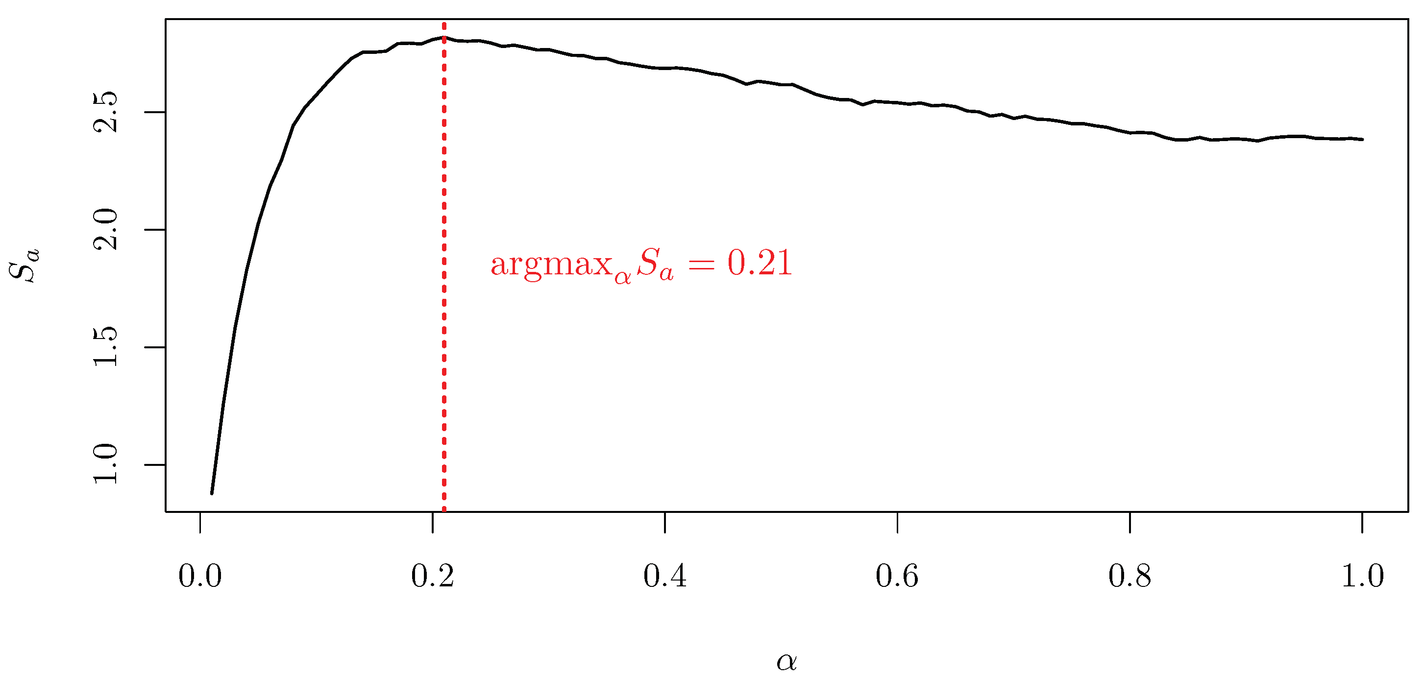
In this section, we jointly apply the concepts introduced in Section 2 and Section 3. Section 4.1 defines an optimization criterion to choose α based on maximizing the risk-adjusted returns. A realistic case study is introduced and investigated in Section 4.2. Section 4.3 discusses the optimal α landscape under different { p i } distributions and considering different values of the target return ϱ .

4.1. α as the Solution of an Optimization Problem

Let us consider a credit insurance company that is regulated by the Solvency 2 framework and adopts the RAF introduced in Section 3. The company’s top management fixes the target return that the line of business must attain in the following fiscal year. The target determines the value of ϱ and, together with the δ SCR ¯ Udw value established by the company’s risk management, implies a risk appetite level per buyer, depending on the buyer’s creditworthiness, through Equation (25). The company’s internal rating system evaluates the creditworthiness level, whose specifications are the ones described in Section 2.
So far, δ SCR ¯ Udw and ϱ allow us to evaluate the C ˜ ( r ) curve. However, it is worth noticing that it holds C ˜ ( r ) > 0 by construction, implying a non-zero risk appetite level for any buyer, regardless of the measured creditworthiness. For practical purposes, we may expect the following deviation from the theoretical curve:
C ˘ ( r ) : = 1 I { r R ˘ } C ˜ ( r )
Namely, a notch R ˘ is associated with the minimum acceptable creditworthiness per buyer. Beyond that level, the insured sellers’ requests for a credit limit are rejected. In Equation (26) and the following, we adopt the convention that creditworthiness decreases as the notch r increases.
Given the RAF introduced above, the optimization problem is finally specified by choice of a objective function that links each α [ 0 , 1 ] to a risk-adjusted returns level attained by the insurer. A natural choice is the Sharpe ratio S a , which in this context can be specified as follows
S a : = ( 1 c ϱ 0 ) Π k i p i C ˘ ( r i ) k i p i ( 1 p i ) C ˘ 2 ( r i ) .
The insurance business’ extra return is obtained by subtracting costs c Π , risk-free returns ϱ 0 Π , and expected loss contribution from the total premiums. However, it is worth noticing that both the expected loss and the loss volatility are estimated by the set { p i } of “actual” PD per buyer. At the same time, each premium contribution π i is implicitly computed by the set { p r ( i ) } of PD per grade, which is available to the insurer after having calibrated the internal rating system. Loss events are assumed to be independent in estimating the loss volatility level needed in the S a definition. Further, it is assumed that the appetite for protection of the insured sellers is generally greater than the insurer capability per debtor, implying the i-th credit limit to be equal to C ˘ ( r i ) .
Thus, the optimal choice for α is the solution
α : = argmax α S a
where S a and the whole RAF implicitly depend on the partitions s ¯ Fix and s ¯ HR , which have to be optimally mixed by α .

4.2. A Full Working Example

We consider a credit insurance company equipped with the internal rating system described in Section 2. The company has to fix α to specify the rating scale through Equation (11). Thus, the problem introduced in Equation (28) must be addressed, given the risk exposures portfolio, the costs, and the target return required by the stakeholders.
The problem’s features are completed by considering the following assumptions. The PDs { p i } are Beta distributed. The company’s rating scale has 10 notches (i.e., “1—highest creditworthiness” to “10—lowest creditworthiness”), following the standards commonly adopted across the credit insurance market [13]. The central PD level p r associated to the r-th notch is defined as
p r : = 1 2 logistic s r 1 ( α ) + logistic s r ( α ) .
This definition is independent of the PD distribution of the r-rated debtors. The main advantage is that there is no need for updating p r as the buyers population evolves, unlike other possible choices, such as
p r : = E p | logit ( p ) [ s r 1 , s r ) .
On the other hand, the drawback is the possible lack of precision in approximating the actual p i associated with each r-rated debtor, especially in case of a wide interval [ s r 1 , s r ) associated with the notch r.
The insurance company’s management fixes the risk appetite δ SCR ¯ Udw , the target return ϱ , the premiums P next to be earned over the next year, and the maximum acceptable notch R ˘ . Conversely, the variables k, , c and D are measurable. Thus, Equations (25), (26) and (29) allow us to fully specify the considered decisional system
C ˘ r ( α ) : = 1 I { r R ˘ } δ SCR ¯ Udw Δ P 1 ϱ c k p r 1 ( α ) .
where Δ P ( P , D ) can be evaluated through Equation (23), recalling that D is measurable, and that P P next .
In Table 1, we provide the specifications of a working example to solve the problem stated in Equation (28) under realistic assumptions.
The fixed-semantics rating scale is chosen a priori, considering a typical Moody’s rating scale as a reference (see, e.g., [14,15,35]). Namely, s ¯ Fix is taken so that p r computed through Equation (29) fits the considered rating scale. Considering a widespread rating scale as the possible fixed-semantics scale of the system is a sounding choice, as the company’s credit analysts and management will likely be familiar with it. The resulting partition is depicted in Figure 1 against the considered buyers’ PD distribution.
The information-based rating scale is chosen a posteriori, considering the PD distribution across the risky buyers’ population. s ¯ HR is estimated as the solution to the problem introduced in Equation (10). The resulting partition is depicted in Figure 2 against the considered buyers’ PD distribution. A comparison between Figure 1 and Figure 2 highlights how s ¯ HR fits the distribution { p i } better than s ¯ Fix . This feature is expected, as s ¯ HR implicitly depends on { p i } through the objective function defined in Equation (8).
Given s ¯ HR and s ¯ Fix , we find the optimal α value to mix the two rating scales according to the RAF introduced above and the set of assumption displayed in Table 1. Without claim to completeness, it is worth noticing that the solution to the problem stated in Equation (28) is nontrivial, in the sense that α 21 % and thus s ¯ ( α ) does not coincide with s ¯ Fix nor with s ¯ HR , as shown in Figure 3.
This result copes with the intuition, as s ¯ Fix is chosen a priori. In contrast, s ¯ HR is the solution to an optimization problem different from the one in Equation (28). In an actuarial perspective, this result suggests that a credit insurance company may somewhat benefit from mixing its a priori rating scale with an information-based rating scale.
The graphical solution to problem in Equation (28) is displayed in Figure 4, where the displayed simulation shows a smooth behavior of the Sharpe ratio S a as a function of α and the existence of one local maximum, which is not located at the boundaries { 0 ; 1 } of the α domain.

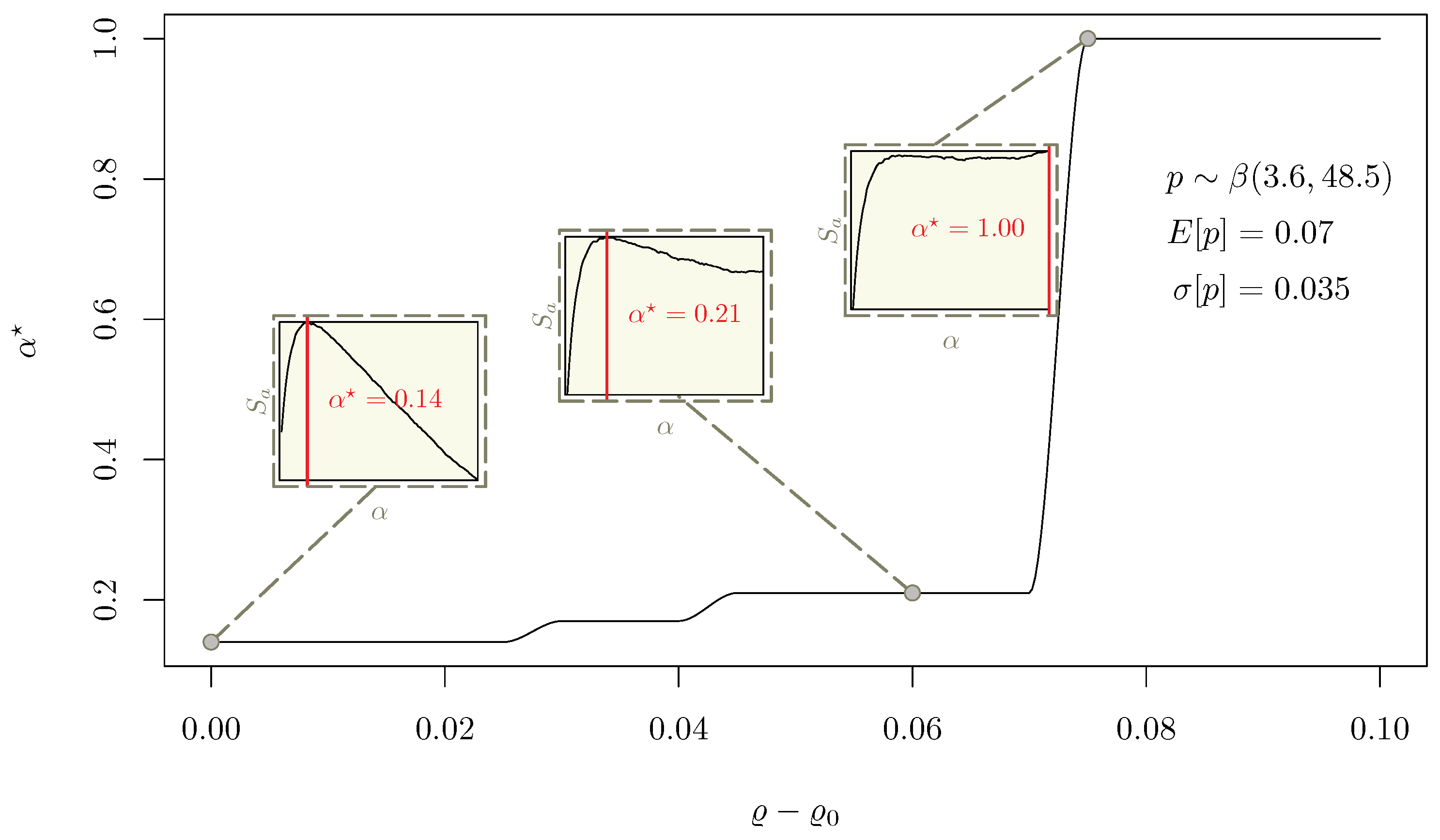
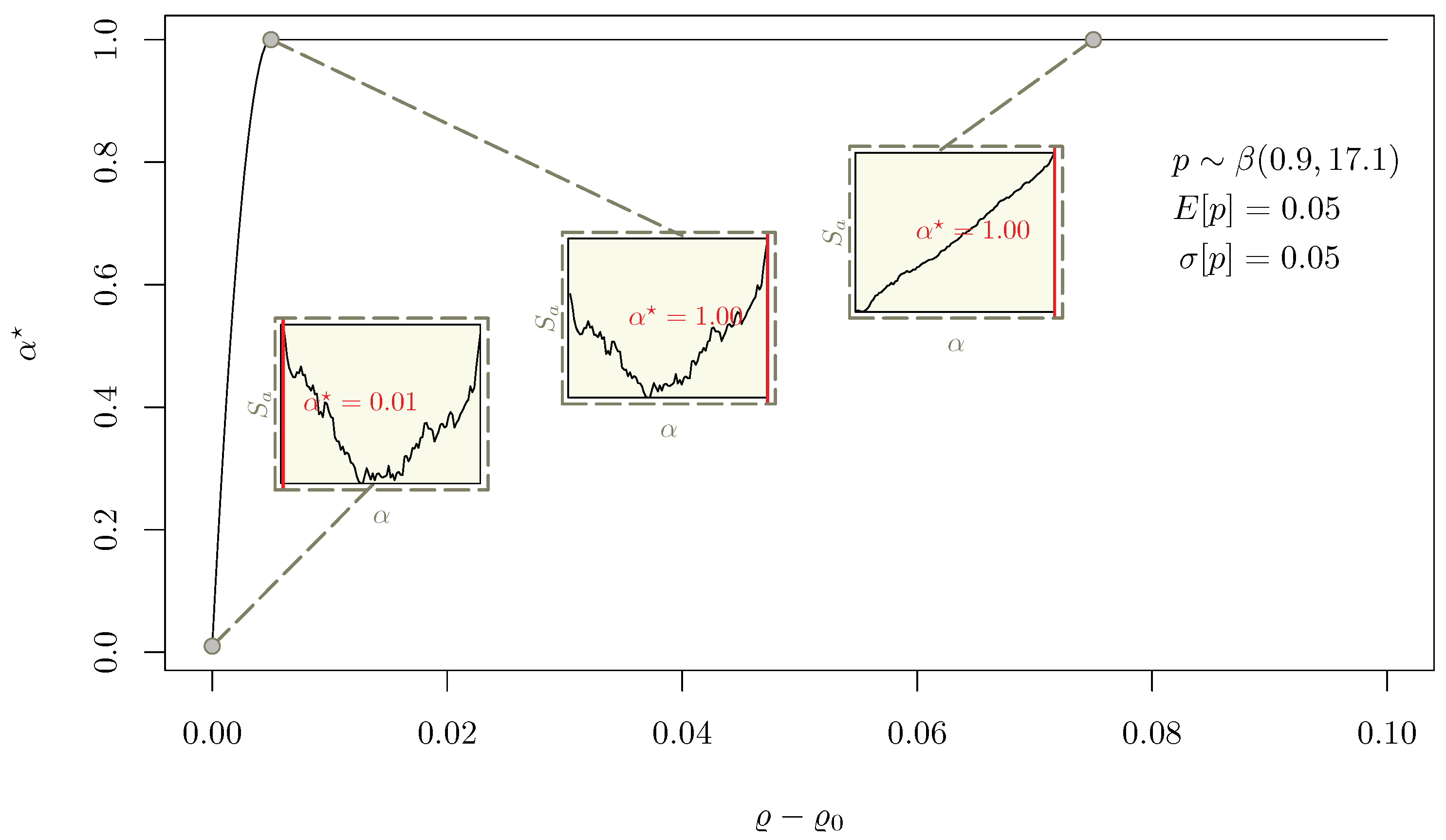
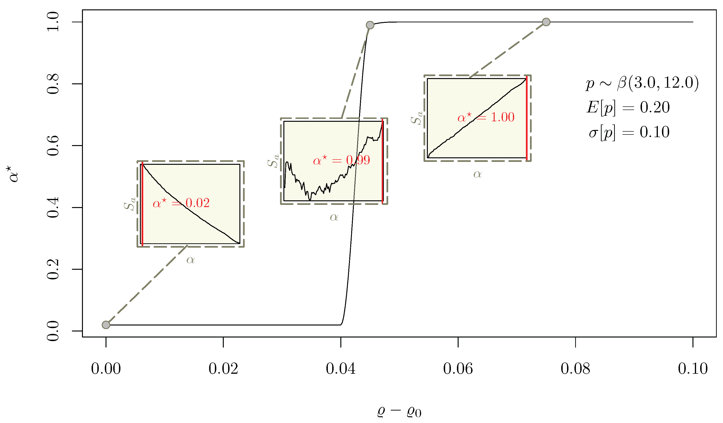
4.3. Sensitivity Analysis

Section 4.2 shows how to choose the optimal α in a realistic, practical case. However, a wide range of realistic setups may be considered instead of the one detailed in Table 1.
Further, the framework itself can be modified. For example, other measures of the risk-adjusted returns can be chosen instead of the Sharpe ratio, or implementation of the Solvency 2 framework based on a partial internal model is feasible instead of the Standard Formula used in Section 3.2. Nonetheless, it is worth noticing that all the possible variations to the considered case study do not affect the possibility nor the interest of identifying and applying a hybrid rating scale that maximizes the risk-adjusted returns of the insurer, while satisfying the constraints imposed by the chosen RAF.
Two elements are considered in the following sensitivity analysis: the target return ϱ requested by the stakeholder and the PD’s distribution of the risky buyers underlying the insurance policies.
Despite the number of variables involved in the RAF definition, this choice is exhaustive due to the functional form of C ˘ r . In fact, the automated decisional system specified in Section 4.1 and Section 4.2 can be represented as the product of two terms, as shown in Equation (31). One of them is inversely proportional to the PD of a considered risky buyer, previously evaluated by the internal rating system of the insurer. The other one is a function of all the elements relevant to the RAF and the capital absorption metrics, including the returns level ϱ . Thus, for each α , exploring the reduced parameters’ space of ϱ and the buyers’ PD distribution, we obtain all the possible C ˘ r ( α ) profiles. Indeed, for the reason above, modifying any other degree of freedom of our system, such as k, , or c, would produce an effect on C ˘ r ( α ) which is perfectly equivalent to the one produced by a specific choice of ϱ , implying that a sensitivity more extended than the one proposed would be redundant.
The proposed sensitivity analysis systematically explores ϱ [ 0.02 , 0.12 ] , given three distinct PD distributions. For each distribution and each ϱ value, the optimization problem defined in Equation (28) is solved separately, obtaining one α ( ϱ ) curve per PD distribution. The three curves are displayed in Figure 5, Figure 6 and Figure 7. Since each point of a α ( ϱ ) is the result of the optimization performed over a S a ( α | ϱ ) curve, each figure features three subplots to show how the S a ( α | ϱ ) profile evolves as a function of ϱ , implying different α solution across the considered domain.
In Figure 5, the optimal α is numerically investigated considering the same set of assumptions reported in Table 1, apart from ϱ , which ranges from 2 % to 12 % , so that the over-risk-free returns range in the 0–10% interval.
A highly non-linear relation links ϱ and S a by construction, as both the decisional system C ˘ r and the premium contribution π i of the i-th buyer depend on ϱ . Thus, finding a nontrivial dependency of the solution α from ϱ ϱ 0 in the considered range 0–10% is not surprising.
Remarkably, Figure 5 shows the existence of a critical threshold of the target return, beyond which it holds α 1 , that is, the s ¯ HR component becomes preponderant in the mix at increasing target returns. Conversely, it holds α tends to zero as ϱ is approaching ϱ 0 , and α ( ϱ ) results to be monotonically increasing across the whole considered domain.
The three subplots in Figure 5 display the distortion of the curve S a ( α | ϱ ) at different ϱ values, providing insight on the α variation as a function of the target return.
The analysis is repeated, considering two alternative distributions of the PDs. The results are displayed in Figure 6 and Figure 7, respectively. The monotonicity of α ( ϱ ) and the existence of a critical threshold ϱ ¯ such that α ( ϱ | ϱ > ϱ ¯ ) 1 are numerically confirmed also in these cases.

5. Conclusions

In this work, we have investigated whether and to what extent applying a hybrid rating scale is beneficial in the non-life insurance risk management context. More precisely, our analyses have been focused on a credit insurance company subject to the Solvency 2 framework. Although considering realistic assumptions, both on the regulatory and the business sides, we have adopted a fully simulative approach to study the specific effects of the hybrid rating scale, excluding any distortion originated by the system’s imperfection (e.g.,: calibration errors in the scoring model underlying the rating system). We have designed a realistic RAF based on the Solvency 2 Standard Formula, where the decisional system grants different credit limits depending on the rating evaluations. Assuming the insurance company aims to maximize its risk-adjusted returns, measured through the Sharpe ratio, we have defined and solved an optimization problem that returns the best hybrid rating scale to choose in order to reach the target returns given all the constraints concerning the capital absorption, the expenses, and the available market.
Since all the considered variables are accessible to a real-world credit insurer, the optimization problem proposed in this work and its solution are of practical interest to the insurance industry. As our results show, a credit insurance company can actually benefit from a hybrid rating scale, and this work provides all the tools needed to identify which choice best suits a specific company.
The numerical results show that the optimal mix strongly depends on the evaluated debtors’ distribution and the unadjusted target returns requested by the stakeholders. Remarkably, our simulations highlight the existence of a critical threshold in target returns, beyond which the information-based master scale is the optimal choice. Conversely, in the presence of relatively low extra returns, a mixed rating scale or even a pure semantics-based master scale is the optimal choice. This is a key result of this paper. A better understanding of the observed critical threshold and its causes could help a credit insurer choose its rating scale even more effectively. In principle, a complete explanation of this phenomenon could lead to a closed-form solution to the proposed optimization problem, with exciting implications both on theoretical and practical sides. The theoretical reasons behind the existence of a critical threshold of returns and, more generally, the nontrivial behavior of the optimal mixing parameter as a function of the target returns are beyond the scope of this work and deserve further investigations in future research works.
This work is limited to studying the interplay between the internal rating system and the risk appetite framework of a credit insurance company, providing a practical toolkit to identify the optimal rating scale. Thus, there is no claim to completeness with respect to the wide range of other practical applications of the hybrid rating scale method and the related optimization problem. However, the investigated application shows the advantage of choosing an optimal rating scale and the necessity to identify it through a rigorous optimization process since it strongly depends on the specific features of the rating model user. The specialization of these methods to other applicative contexts could be addressed in the future as a development of the presented research activity.

Funding

This research received no external funding.

Data Availability Statement

Not applicable.

Conflicts of Interest

The author declares no conflict of interest.

References

  1. Hodgetts, T.J.; Hall, J.; Maconochie, I.; Smart, C. Paediatric triage tape. Prehosp. Immed. Care 2013, 2, 155–159. [Google Scholar]
  2. Cross, K.P.; Cicero, M.X. Head-to-head comparison of disaster triage methods in pediatric, adult, and geriatric patients. Ann. Emerg. Med. 2013, 61, 668–676. [Google Scholar] [CrossRef] [PubMed]
  3. Lerner, E.B.; McKee, C.H.; Cady, C.E.; Cone, D.C.; Colella, M.R.; Cooper, A.; Coule, P.L.; Lairet, J.R.; Liu, J.M.; Pirrallo, R.G.; et al. A consensus-based gold standard for the evaluation of mass casualty triage systems. Prehosp. Emerg. Care 2015, 19, 267–271. [Google Scholar] [CrossRef]
  4. Elo, A.E. The Proposed USCF Rating System. Chess Life 1967, XXII, 242–247. Available online: http://uscf1-nyc1.aodhosting.com/CL-AND-CR-ALL/CL-ALL/1967/1967_08.pdf (accessed on 6 June 2023).
  5. Glickman, M.E. Parameter estimation in large dynamic paired comparison experiments. Appl. Stat. 1999, 48, 377–394. [Google Scholar] [CrossRef]
  6. Veček, N.; Mernik, M.; Črepinšek, M.; Hrnčič, D. A Comparison between Different Chess Rating Systems for Ranking Evolutionary Algorithms. In Proceedings of the 2014 Federated Conference on Computer Science and Information Systems, Warsaw, Poland, 7–10 September 2014. [Google Scholar]
  7. Thurstone, L.L. Theory of attitude measurement. Psychol. Rev. 1929, 36, 222. [Google Scholar] [CrossRef]
  8. Likert, R. A technique for the measurement of attitudes. Arch. Psychol. 1932, 22, 55. [Google Scholar]
  9. Parducci, A. Category ratings and the relational character of judgment. Adv. Psychol. 1983, 11, 262–282. [Google Scholar]
  10. Menold, N.; Wolf, C.; Bogner, K. Design aspects of rating scales in questionnaires. Math. Popul. Stud. 2018, 25, 63–65. [Google Scholar] [CrossRef]
  11. Carlsen, L. Rating Potential Land Use Taking Ecosystem Service into Account—How to Manage Trade-Offs. Standards 2021, 1, 79–89. [Google Scholar] [CrossRef]
  12. Weissova, I.; Kollarb, B.; Siekelova, A. Rating as a Useful Tool for Credit Risk Measurement. Procedia Econ. Financ. 2015, 26, 278–285. [Google Scholar] [CrossRef]
  13. European Insurance and Occupational Pensions Authority—EIOPA. NLCS 2020 log File A, (V1.1) Updated on 19 July 2021. Available online: https://www.eiopa.europa.eu/consultations/non-life-underwriting-risk-comparative-study-internal-models_en (accessed on 6 June 2023).
  14. Güttler, A.; Raupach, P. The Impact of Downward Rating Momentum on Credit Portfolio Risk; Discussion Paper Series 2: Banking and Financial Studies No° 16/2008 Deutsche Bundesbank. Available online: https://www.bundesbank.de/resource/blob/704272/d4c8a1578e3122b5cfe696e0553865c3/mL/2008-06-24-dkp-16-data.pdf (accessed on 6 June 2023).
  15. Rating Symbols and Definitions. Moody’s Investors Service, 2 June 2022. Available online: https://www.moodys.com/researchdocumentcontentpage.aspx?docid=pbc_79004 (accessed on 6 June 2023).
  16. Oosterveld, B.; Bauer, S. Rating Definitions. FitchRatings Special Report, 21 March 2022. Available online: https://www.fitchratings.com/research/structured-finance/rating-definitions-21-03-2022 (accessed on 6 June 2023).
  17. Nehrebecka, N. Probability-of-default curve calibration and validation of internal rating systems. In Proceedings of the 8th IFC Conference on “Statistical Implications of the New Financial Landscape”, Basel, Switzerland, 8–9 September 2016; Available online: https://www.bis.org/ifc/publ/ifcb43_zd.pdf (accessed on 6 June 2023).
  18. Giacomelli, J. The Rating Scale Paradox: Semantics Instability versus Information loss. Standards 2022, 2, 352–365. [Google Scholar] [CrossRef]
  19. Frei, C. and Wunsch, M. Moment Estimators for Autocorrelated Time Series and Their Application to Default Correlations. J. Credit. Risk 2018, 14, 1–29. Available online: https://ssrn.com/abstract=3141168 (accessed on 30 September 2023). [CrossRef]
  20. Gordy, M.B. and Howells, B. Procyclicality in Basel II: Can we treat the disease without killing the patient? J. Financ. Intermediation 2006, 15, 395–417. [Google Scholar] [CrossRef]
  21. Altman, E.I.; Rijken, H.A. How rating agencies achieve rating stability. J. Bank. Financ. 2004, 28, 2679–2714. [Google Scholar] [CrossRef]
  22. Cantor, R.M.; Mann, C. Analyzing the Tradeoff between Ratings Accuracy and Stability. J. Fixed Income 2006. Available online: https://ssrn.com/abstract=996019 (accessed on 30 September 2023). [CrossRef]
  23. Giacomelli, J. Parametric estimation of latent default frequency in credit insurance. J. Oper. Res. Soc. 2023, 74, 330–350. [Google Scholar] [CrossRef]
  24. The International Credit Insurance & Surety Association. A Guide to Trade Credit Insurance; Anthem Press: London, UK, 2015. [Google Scholar]
  25. The International Credit Insurance & Surety Association. ICISA Catalog of Credit Insurance Terminology—English Edition. 2017. Available online: icisa.org/wp-content/uploads/2019/07/ICISA-Catalogue-of-Credit-Insurance-Terminology-English.pdf (accessed on 6 June 2023).
  26. Jus, M. Credit Insurance; Academic Press: Cambridge, MA, USA, 2013. [Google Scholar]
  27. Passalacqua, L. A pricing model for credit insurance. G. Dell’Istituto Ital. Degli Attuari 2006, 69, 4. [Google Scholar]
  28. Passalacqua, L. Measuring effects of excess-of-loss reinsurance on credit insurance risk capital. Giornale Dell’Istituto Ital. Degli Attuari 2007, 70, 81–102. [Google Scholar]
  29. Commission Delegated Regulation (EU) 2015/35 of 10 October 2014 Supplementing Directive 2009/138/EC of the European Parliament and of the Council on the Taking-Up and Pursuit of the Business of Insurance and Reinsurance. Available online: https://eur-lex.europa.eu/eli/reg_del/2015/35/oj (accessed on 6 June 2023).
  30. Commission Delegated Regulation (EU) 2019/981 of 8 March 2019 Amending Delegated Regulation (EU) 2015/35 Supplementing Directive 2009/138/EC of the European Parliament and of the Council on the Taking-Up and Pursuit of the Business of Insurance and Reinsurance (Solvency II). Available online: https://eur-lex.europa.eu/eli/reg_del/2019/981/oj (accessed on 6 June 2023).
  31. Directive 2009/138/EC of the European Parliament and of the Council of 25 November 2009. Available online: https://eur-lex.europa.eu/eli/dir/2009/138/oj (accessed on 6 June 2023).
  32. Stanghellini, E. Introduzione ai Metodi Statistici per il Credit Scoring, 1st ed.; Springer: Berlin/Heidelberg, Germany, 2009. [Google Scholar]
  33. Konrad, P.M. The Calibration of Rating Models. Estimation of the Probability of Default based on Advanced Pattern Classification Methods, 1st ed.; Tectum Verlag Marburg: Marburg, Germany, 2012. [Google Scholar]
  34. Gurný, P.; Gurný, M. Comparison of credit scoring models on probability of defaults estimation for US banks. Prague Econ. Pap. 2013, 22, 163–181. [Google Scholar] [CrossRef]
  35. Fankenstein, E.; Boral, A.; Carty, L.V. RiskCalc for Private Companies: Moody’s Default Model. Moody’s Investor Service Global Credit Research, May 2000. Available online: https://ssrn.com/abstract=236011 (accessed on 6 July 2023).
  36. Basel Committee on Banking Supervision (BSBC). The Internal Ratings-Based Approach; Bank for International Settlements: Basel, Switzerland, 2001. [Google Scholar]
  37. Tasche, D. The art of probability-of-default curve calibration. J. Credit. Risk 2013, 9, 63–103. [Google Scholar] [CrossRef]
  38. Durović, A. Macroeconomic Approach to Point in Time Probability of Default Modeling—IFRS 9 Challenges. J. Cent. Bank. Theory Pract. 2019, 1, 209–223. [Google Scholar] [CrossRef]
  39. Fawcett, T. An introduction to ROC analysis. Pattern Recognit. Lett. 2006, 27, 861–874. [Google Scholar] [CrossRef]
  40. Engelmann, B.; Hayden, E.; Tasche, D. Measuring the Discriminative Power of Rating Systems; Discussion Paper Series 2: Banking and Financial Supervision No 01/2003 Deutsche Bundesbank. Available online: https://www.bundesbank.de/resource/blob/704150/b9fa10a16dfff3c98842581253f6d141/mL/2003-10-01-dkp-01-data.pdf (accessed on 6 June 2023).
  41. Giacomelli, J.; Passalacqua, L. Unsustainability Risk of Bid Bonds in Public Tenders. Mathematics 2021, 9, 2385. [Google Scholar] [CrossRef]
  42. Giacomelli, J.; Passalacqua, L. Calibrating the CreditRisk+ Model at Different Time Scales and in Presence of Temporal Autocorrelation. Mathematics 2021, 9, 1679. [Google Scholar] [CrossRef]
  43. Giacomelli, J.; Passalacqua, L. Improved precision in calibrating CreditRisk+ model for Credit Insurance applications. In Mathematical and Statistical Methods for Actuarial Sciences and Finance—eMAF 2020; Springer International Publishing: Berlin/Heidelberg, Germany, 2021. [Google Scholar] [CrossRef]
  44. Paulusch, J. The Solvency II Standard Formula, Linear Geometry, and Diversification. J. Risk Financ. Manag. 2017, 10, 11. [Google Scholar] [CrossRef]
  45. Baione, F.; De Angelis, P.; Granito, I. On a Capital Allocation Principle Coherent with the Solvency 2 Standard Formula. IVASS Conference on Insurance Research, 13 July 2017. Available online: https://www.ivass.it/pubblicazioni-e-statistiche/pubblicazioni/att-sem-conv/2017/conf-131407/ (accessed on 6 June 2023).
Figure 1. Semantics-based rating scale (i.e., α = 0 ) compared with the buyers’ PD distribution β ( 3.6 , 48.5 ) specified in Table 1, considering a population of 10 5 individuals. The amplitude of each colored band highlights the PD interval associated with a given notch r of the rating scale, from lower PDs (green band, corresponding to r = 1 ) to higher PDs (red band, corresponding to r = 10 ).
Standards 03 00025 g001
Figure 2. Information-based rating scale (i.e., α = 1 ) compared with the buyers’ PD distribution β ( 3.6 , 48.5 ) specified in Table 1, considering a population of 10 5 individuals. The interpretation of the colored bands overlying the PD distribution is the same as Figure 1.
Standards 03 00025 g002
Figure 3. Optimal hybrid rating scale (i.e., α = 0.21 ) compared with the buyers’ PD distribution β ( 3.6 , 48.5 ) specified in Table 1, considering a population of 10 5 individuals. The interpretation of the colored bands overlying the PD distribution is the same as Figure 1.
Standards 03 00025 g003
Figure 4. Sharpe ratio as a function of α , considering ϱ = 8 % .
Standards 03 00025 g004
Figure 5. The optimal α : = argmax α S a as a function of the extra-return ϱ ϱ 0 , given the other assumptions in Table 1. The buyer’s PDs { p i } are distributed as a Beta r.v. with parameters α 3.6 and β 48.5 , that copes with the assumptions stated in in Table 1 with specific reference the expected value and the standard deviation of p i .
Standards 03 00025 g005
Figure 6. The optimal α : = argmax α S a as a function of the extra-return ϱ ϱ 0 , given the other assumptions in Table 1. The buyer’s PDs { p i } are distributed as a Beta r.v. with parameters α 0.9 and β 17.1 . This choice corresponds to E p i = 5 % and sd p i = 5 % . The other assumptions needed are chosen as displayed in Table 1.
Standards 03 00025 g006
Figure 7. The optimal α : = argmax α S a as a function of the extra-return ϱ ϱ 0 , given the other assumptions in Table 1. The buyer’s PDs { p i } are distributed as a Beta r.v. with parameters α 0.9 and β 17.1 . This choice corresponds to E p i = 20 % and sd p i = 10 % . The other assumptions needed are chosen as displayed in Table 1.
Standards 03 00025 g007
Table 1. Numerical setup considered as a case study to solve the optimal master scale problem.
VariableDescriptionValue
PPremiums to be earned during the next 12 months (arbitrary units) 10 4
DSCR associated to Catastrophe Default risk in Solvency 2 Standard Formula framework (arbitrary units) 10 3
δ SCR ¯ Udw Risk appetite per risk expressed as the maximum acceptable contribution to the SCR Udw ( SCR Udw units)5 × 10 5
kAverage effect of contractual clauses and conditions 90 %
Average exposure at default ratio 50 %
cInsurer’s cost ratio 35 %
ϱ Target return required by the insurer’s stakeholders 8 %
ϱ 0 Risk free return 2 %
RNumber of notches belonging to the considered master scale10
R ˘ Notch associated with the minimum acceptable creditworthiness per buyer7
NNumber of risky buyers against whom the insured sellers ask for protection 10 5
E p Expected value of the buyers’ PD distribution 7.0 %
sd p Standard deviation of the buyers’ PD distribution 3.5 %
Disclaimer/Publisher’s Note: The statements, opinions and data contained in all publications are solely those of the individual author(s) and contributor(s) and not of MDPI and/or the editor(s). MDPI and/or the editor(s) disclaim responsibility for any injury to people or property resulting from any ideas, methods, instructions or products referred to in the content.

