
Efficient and Accurate 3D Thickness Measurement in Vessel Wall Imaging: Overcoming Limitations of 2D Approaches Using the Laplacian Method
 , , , , , , and
Abstract
:1. Introduction
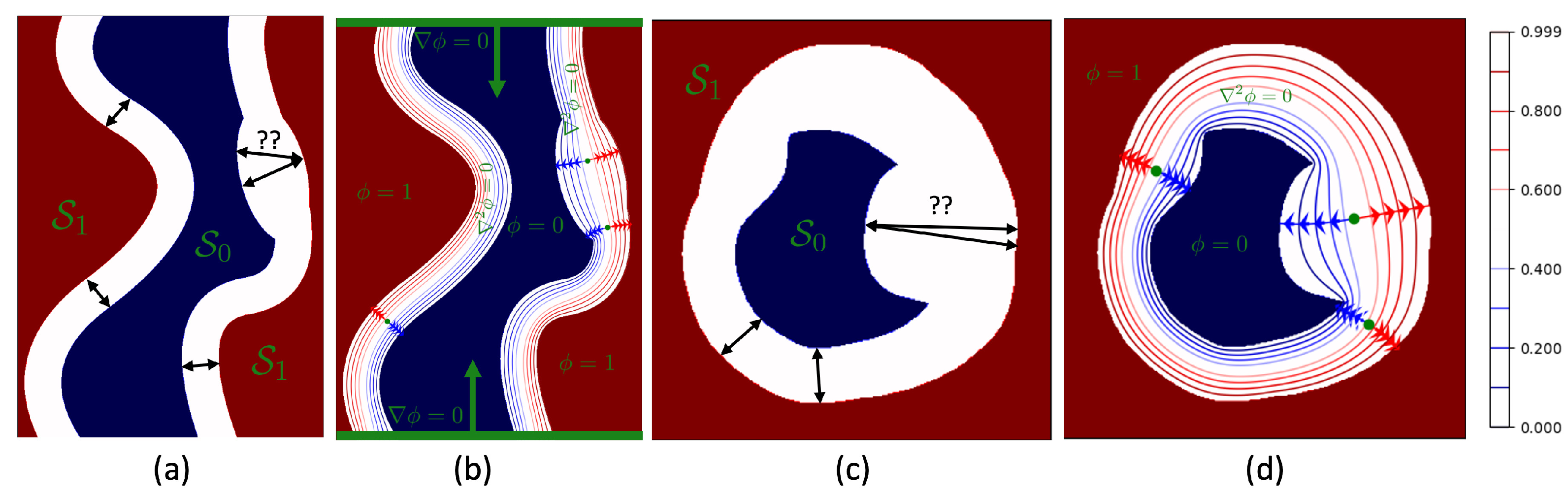
2. Theory
| Algorithm 1: Computing the thickness |
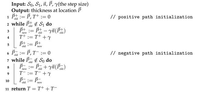 |
| Algorithm 2: Solving the Laplace’s equation using convolutions |
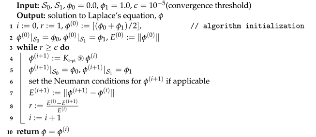 |
3. Materials and Methods
3.1. Thickness Measurement of 2D Digital Phantoms
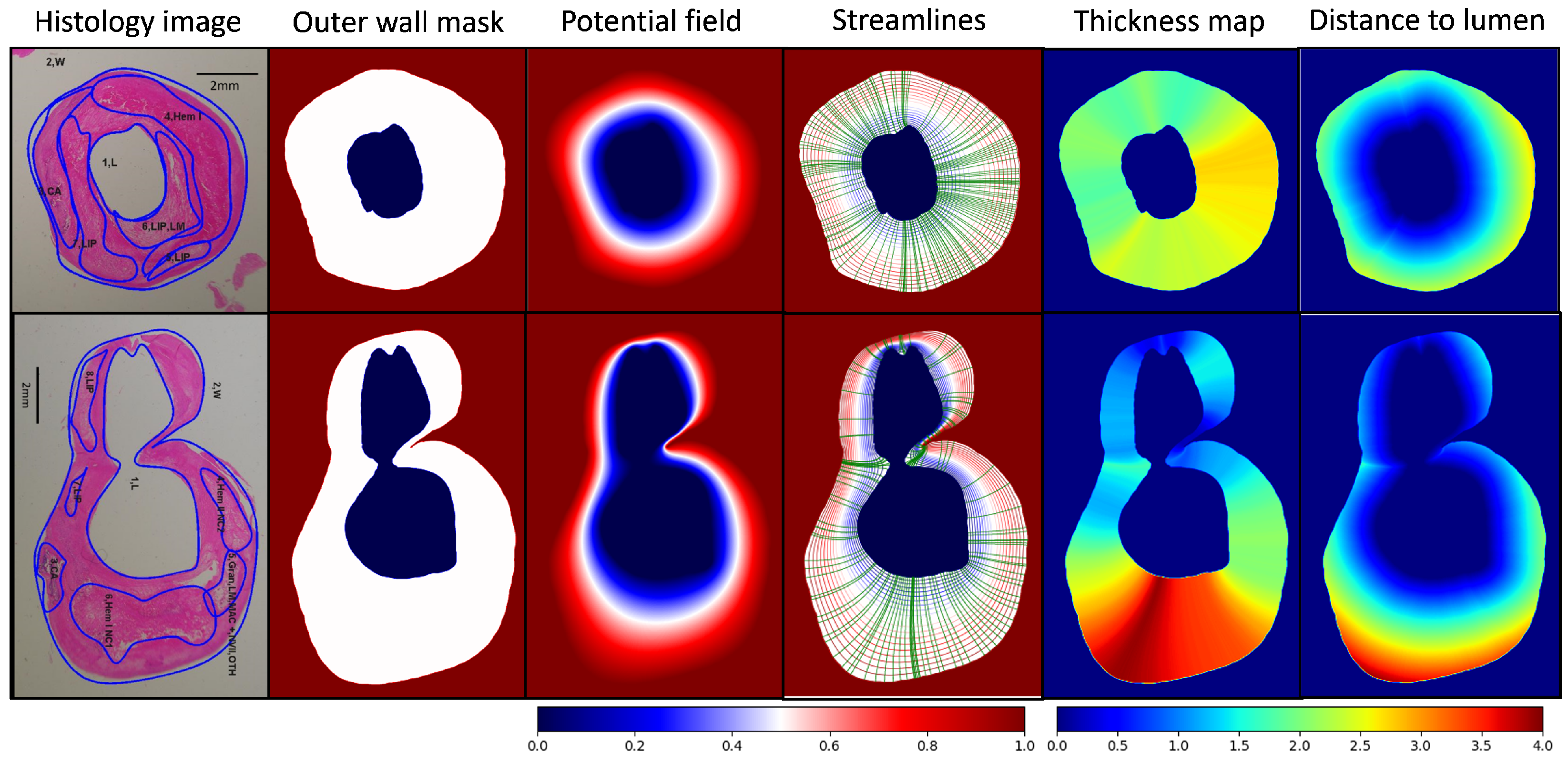
3.2. Outer Wall Thickness Measurement in 2D Histology Images
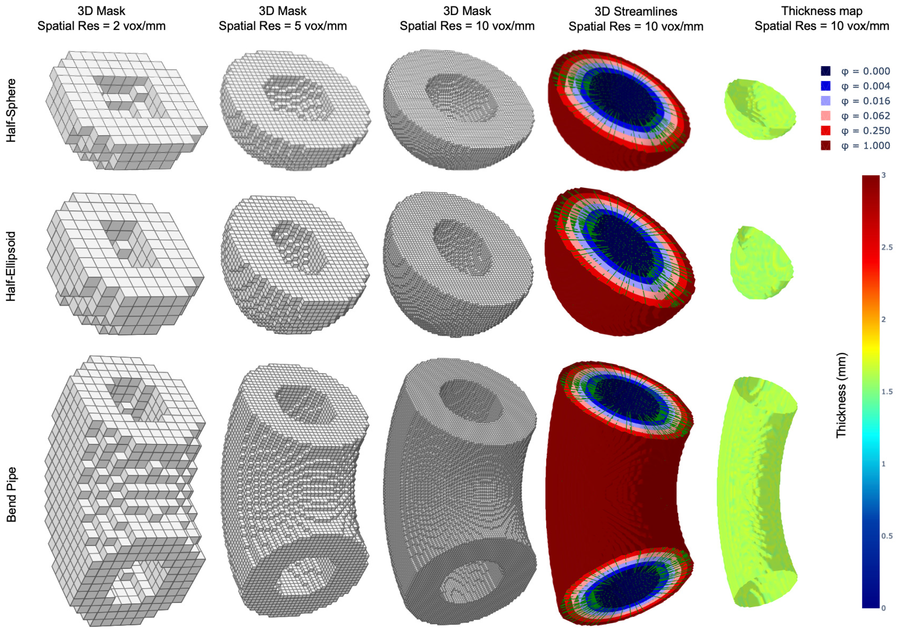
3.3. Thickness Measurements of 3D Digital Phantoms
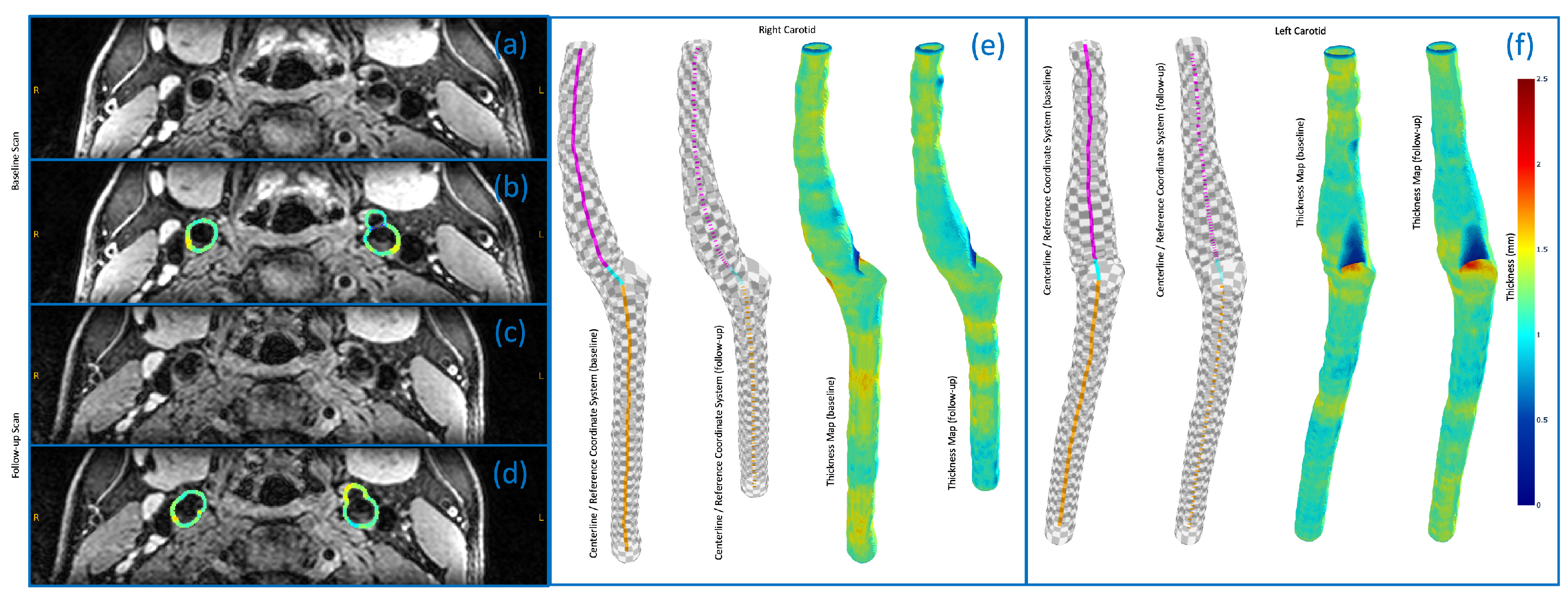
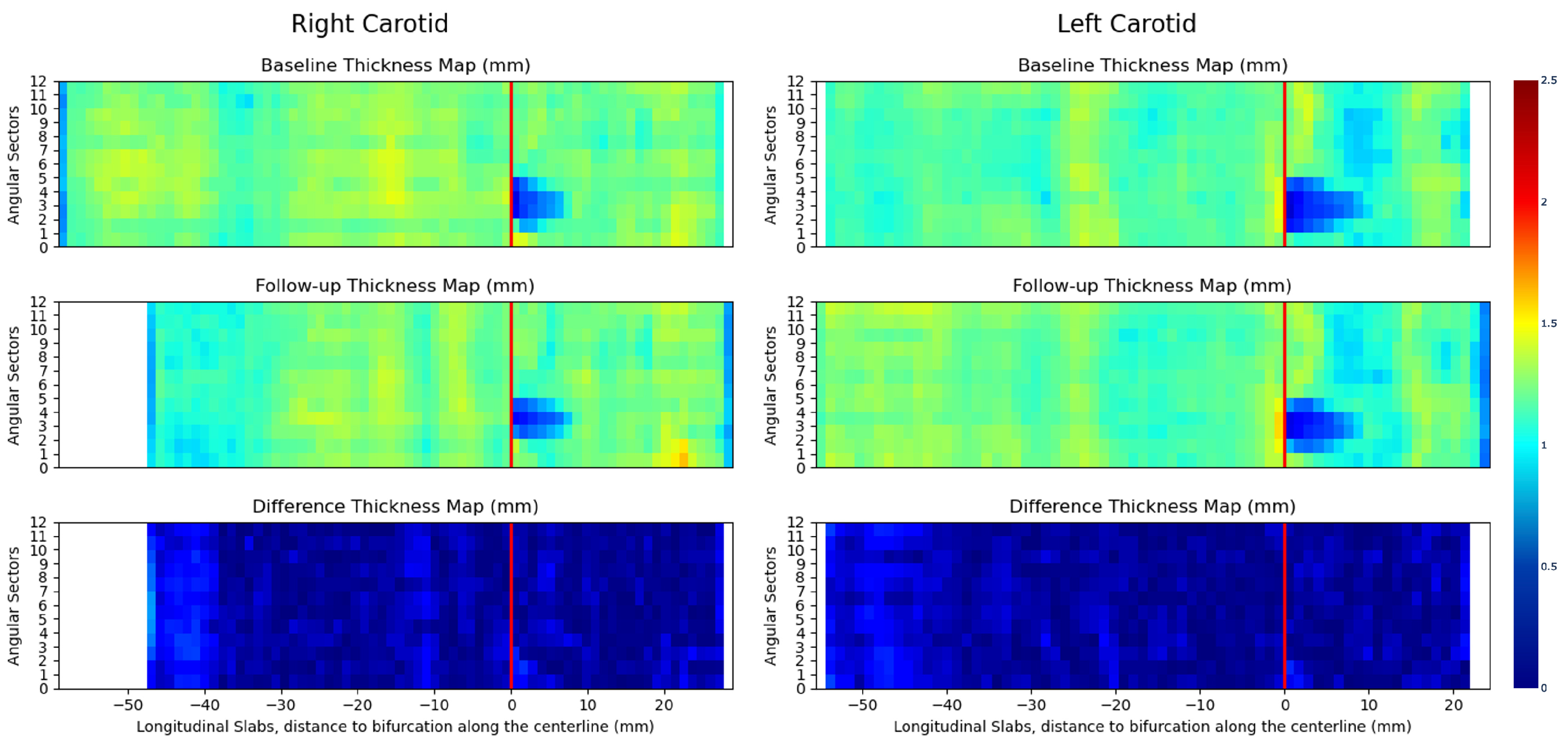
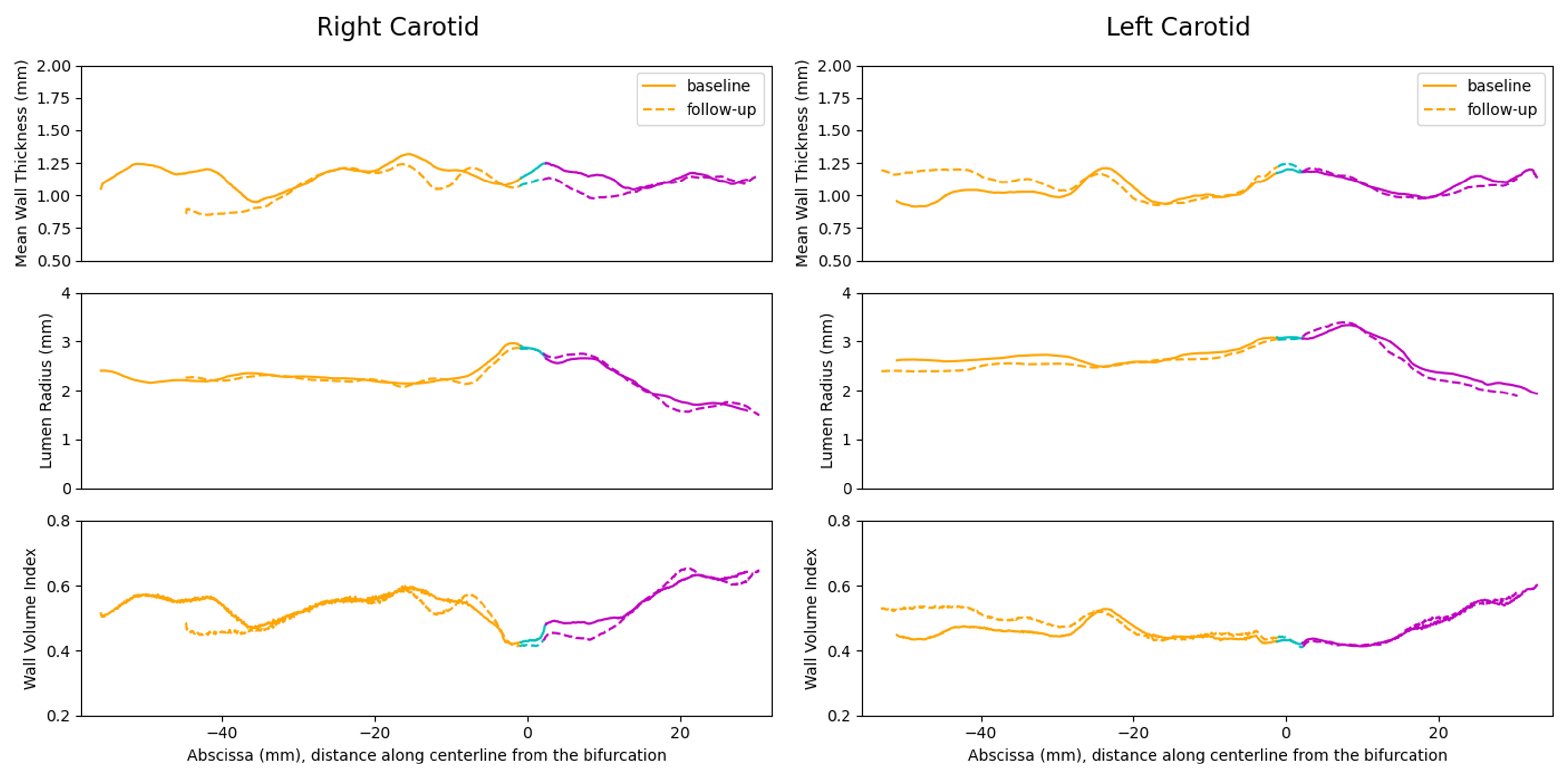
3.4. 3D Vessel Wall Thickness Measurement of Carotid Arteries in Black Blood MR Images
4. Results
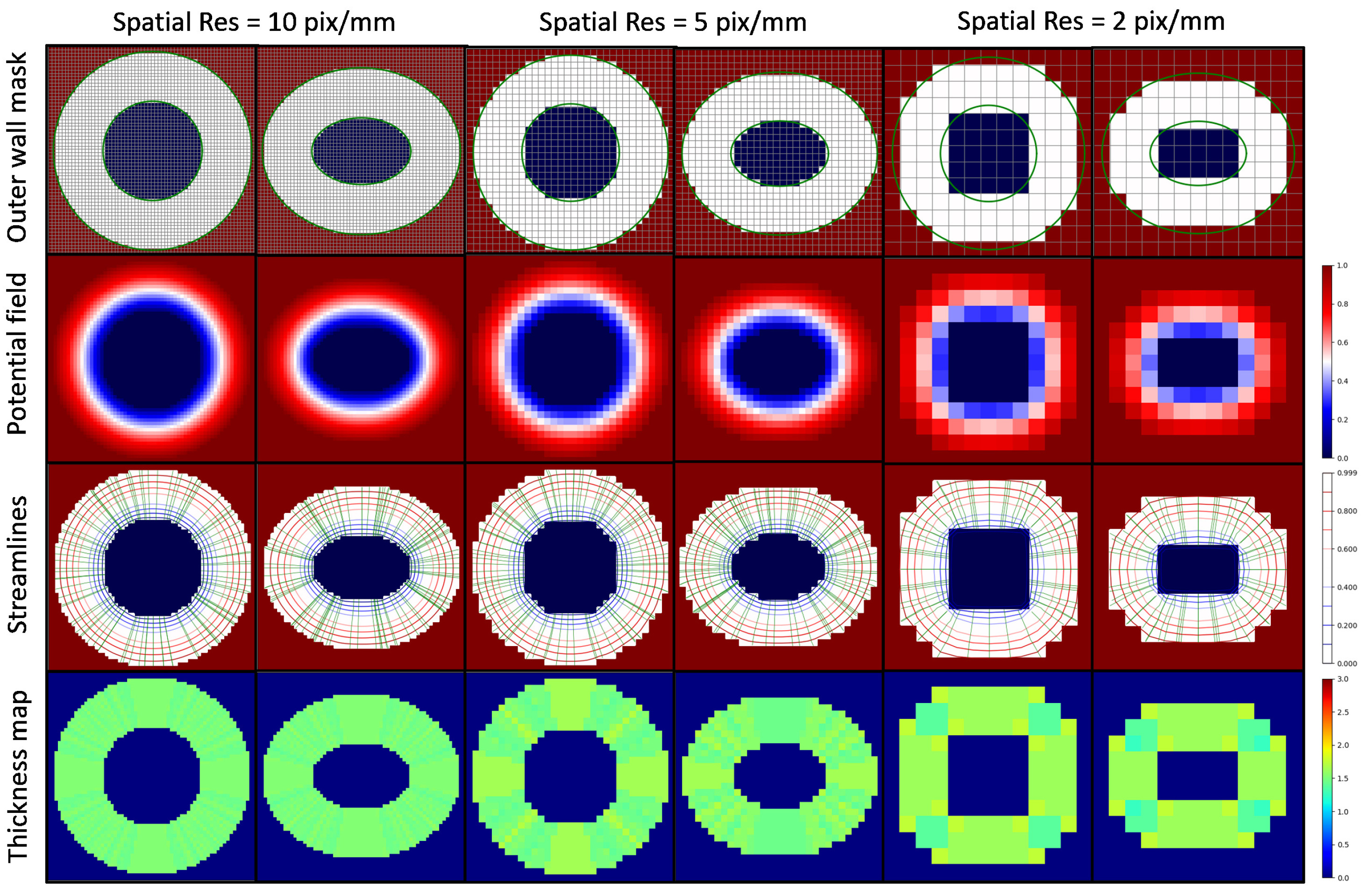
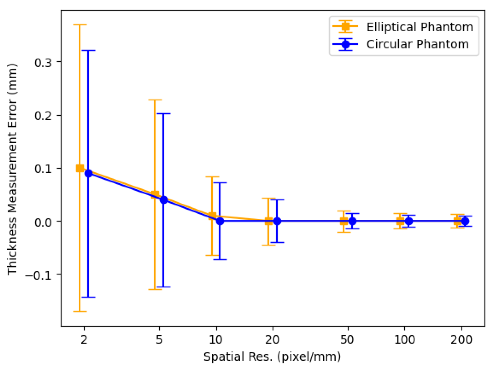
4.1. Thickness Measurement of 2D Digital Phantoms
4.2. Outer Wall Thickness Measurement in 2D Histology Images
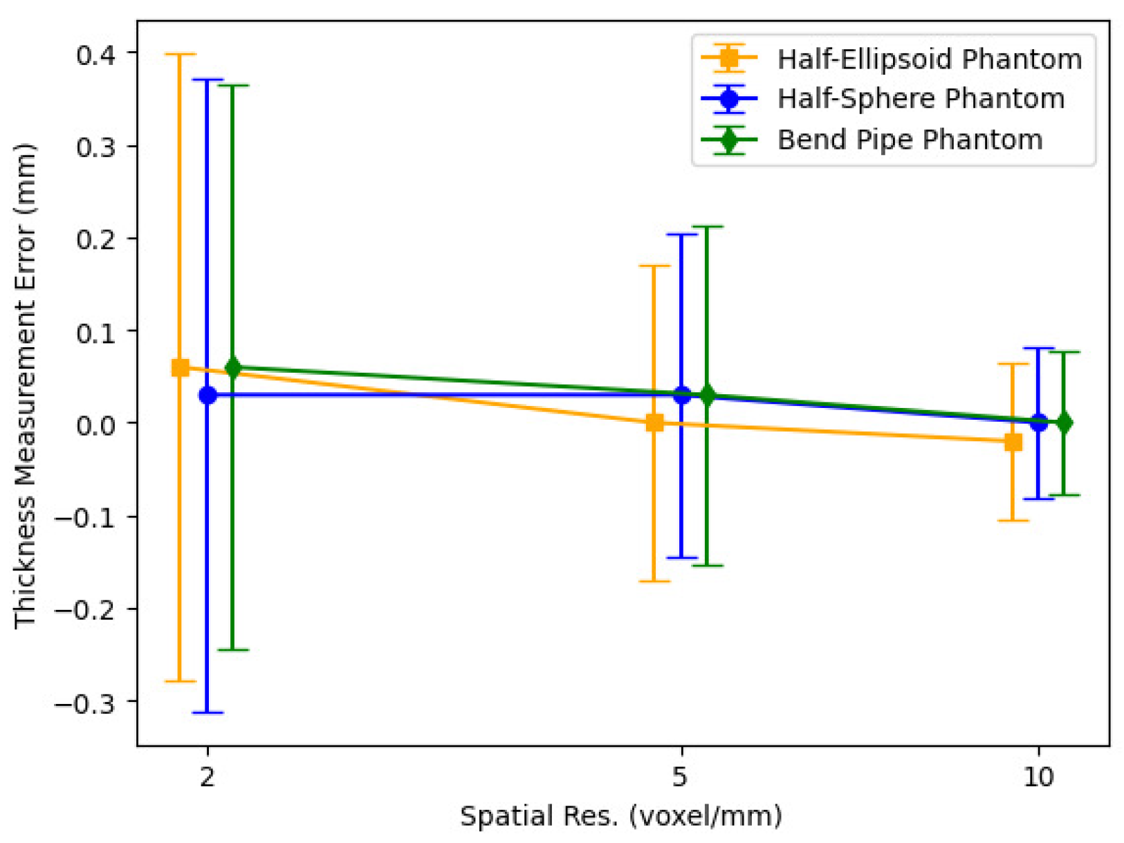
4.3. Thickness Measurements of 3D Digital Phantoms
4.4. 3D Vessel Wall Thickness Measurement of Carotid Arteries in Black Blood MR Images
5. Discussion
6. Conclusions
Supplementary Materials
Author Contributions
Funding
Institutional Review Board Statement
Informed Consent Statement
Data Availability Statement
Acknowledgments
Conflicts of Interest
Abbreviations
| 2D | Two-dimensional |
| 3D | Three-dimensional |
| MRI | Magnetic resonance imaging |
| DL | Deep learning |
| GPU | Graphics processing unit |
| ROI | Region of interest |
| CCA | Common carotid artery |
| ICA | Internal carotid artery |
| H&E | Hematoxylin and eosin |
| IRB | institutional review board |
| 3T | Three Tesla |
| 3D-MERGE | 3D motion-sensitized rapid gradient echo |
| FOV | Field of view |
| AI | Artificial intelligence |
| VMTK | Vascular modeling toolkit |
| SNR | Signal-to-noise ratio |
Appendix A. Extension to 3D
Appendix B. More Robust Kernels
References
- Hodis, H.N.; Mack, W.J.; LaBree, L.; Selzer, R.H.; Liu, C.-R.; Liu, C.-H.; Azen, S.P. The Role of Carotid Arterial Intima-Media Thickness in Predicting Clinical Coronary Events. Ann. Intern. Med. 1998, 128, 262–269. [Google Scholar] [CrossRef] [PubMed]
- O’Leary, D.H.; Polak, J.F.; Kronmal, R.A.; Manolio, T.A.; Burke, G.L.; Wolfson, S.K. Carotid-Artery Intima and Media Thickness as a Risk Factor for Myocardial Infarction and Stroke in Older Adults. N. Engl. J. Med. 1999, 340, 14–22. [Google Scholar] [CrossRef] [PubMed]
- Spence, J.D.; Eliasziw, M.; DiCicco, M.; Hackam, D.G.; Galil, R.; Lohmann, T. Carotid Plaque Area. Stroke 2002, 33, 2916–2922. [Google Scholar] [CrossRef] [PubMed]
- Lorenz, M.W.; Markus, H.S.; Bots, M.L.; Rosvall, M.; Sitzer, M. Prediction of Clinical Cardiovascular Events with Carotid Intima-Media Thickness. Circulation 2007, 115, 459–467. [Google Scholar] [CrossRef]
- Stein, J.H.; Korcarz, C.E.; Hurst, R.T.; Lonn, E.; Kendall, C.B.; Mohler, E.R.; Najjar, S.S.; Rembold, C.M.; Post, W.S. Use of Carotid Ultrasound to Identify Subclinical Vascular Disease and Evaluate Cardiovascular Disease Risk: A Consensus Statement from the American Society of Echocardiography Carotid Intima-Media Thickness Task Force Endorsed by the Society for Vascular Medicine. J. Am. Soc. Echocardiogr. 2008, 21, 93–111. [Google Scholar] [CrossRef]
- Polak, J.F.; Pencina, M.J.; Pencina, K.M.; O’Donnell, C.J.; Wolf, P.A.; D’Agostino, R.B. Carotid-Wall Intima–Media Thickness and Cardiovascular Events. N. Engl. J. Med. 2011, 365, 213–221. [Google Scholar] [CrossRef] [PubMed]
- Baldassarre, D.; Hamsten, A.; Veglia, F.; de Faire, U.; Humphries, S.E.; Smit, A.J.; Giral, P.; Kurl, S.; Rauramaa, R.; Mannarino, E.; et al. Measurements of Carotid Intima-Media Thickness and of Interadventitia Common Carotid Diameter Improve Prediction of Cardiovascular Events: Results of the IMPROVE (Carotid Intima Media Thickness IMT and IMT-Progression as Predictors of Vascular Events in a High Risk European Population) Study. J. Am. Coll. Cardiol. 2012, 60, 1489–1499. [Google Scholar] [CrossRef] [PubMed]
- Touboul, P.J.; Hennerici, M.; Meairs, S.; Adams, H.; Amarenco, P.; Bornstein, N.; Csiba, L.; Desvarieux, M.; Ebrahim, S.; Hernandez Hernandez, R.; et al. Mannheim Carotid Intima-Media Thickness and Plaque Consensus (2004–2006–2011): An Update on Behalf of the Advisory Board of the 3rd, 4th and 5th Watching the Risk Symposia, at the 13th, 15th and 20th European Stroke Conferences, Mannheim, Germany, 2004, Brussels, Belgium, 2006, and Hamburg, Germany, 2011. Cerebrovasc. Dis. 2012, 34, 290–296. [Google Scholar] [CrossRef]
- Bots, M.L.; Groenewegen, K.A.; Anderson, T.J.; Britton, A.R.; Dekker, J.M.; Engström, G.; Evans, G.W.; de Graaf, J.; Grobbee, D.E.; Hedblad, B.; et al. Common Carotid Intima-Media Thickness Measurements Do Not Improve Cardiovascular Risk Prediction in Individuals With Elevated Blood Pressure. Hypertension 2014, 63, 1173–1181. [Google Scholar] [CrossRef]
- Pignoli, P.; Tremoli, E.; Poli, A.; Oreste, P.; Paoletti, R. Intimal plus medial thickness of the arterial wall: A direct measurement with ultrasound imaging. Circulation 1986, 74, 1399–1406. [Google Scholar] [CrossRef]
- Wofford, J.L.; Kahl, F.R.; Howard, G.R.; McKinney, W.M.; Toole, J.F.; Crouse, J.R. Relation of extent of extracranial carotid artery atherosclerosis as measured by B-mode ultrasound to the extent of coronary atherosclerosis. Arterioscler. Thromb. J. Vasc. Biol. 1991, 11, 1786–1794. [Google Scholar] [CrossRef] [PubMed]
- Underhill, H.R.; Kerwin, W.S.; Hatsukami, T.S.; Yuan, C. Automated measurement of mean wall thickness in the common carotid artery by MRI: A comparison to intima-media thickness by B-mode ultrasound. J. Magn. Reson. Imaging 2006, 24, 379–387. [Google Scholar] [CrossRef] [PubMed]
- Harloff, A.; Zech, T.; Frydrychowicz, A.; Schumacher, M.; Schöllhorn, J.; Hennig, J.; Weiller, C.; Markl, M. Carotid intima-media thickness and distensibility measured by MRI at 3T versus high-resolution ultrasound. Eur. Radiol. 2009, 19, 1470–1479. [Google Scholar] [CrossRef] [PubMed]
- Harteveld, A.A.; Denswil, N.P.; Van Hecke, W.; Kuijf, H.J.; Vink, A.; Spliet, W.G.; Daemen, M.J.; Luijten, P.R.; Zwanenburg, J.J.; Hendrikse, J.; et al. Ex vivo vessel wall thickness measurements of the human circle of Willis using 7T MRI. Atherosclerosis 2018, 273, 106–114. [Google Scholar] [CrossRef] [PubMed]
- Balu, N.; Yarnykh, V.L.; Chu, B.; Wang, J.; Hatsukami, T.; Yuan, C. Carotid plaque assessment using fast 3D isotropic resolution black-blood MRI. Magn. Reson. Med. 2011, 65, 627–637. [Google Scholar] [CrossRef] [PubMed]
- Qiao, Y.; Steinman, D.A.; Qin, Q.; Etesami, M.; Schär, M.; Astor, B.C.; Wasserman, B.A. Intracranial arterial wall imaging using three-dimensional high isotropic resolution black blood MRI at 3.0 Tesla. J. Magn. Reson. Imaging 2011, 34, 22–30. [Google Scholar] [CrossRef] [PubMed]
- Li, M.L.; Xu, Y.Y.; Hou, B.; Sun, Z.Y.; Zhou, H.L.; Jin, Z.Y.; Feng, F.; Xu, W.H. High-resolution intracranial vessel wall imaging using 3D CUBE T1 weighted sequence. Eur. J. Radiol. 2016, 85, 803–807. [Google Scholar] [CrossRef] [PubMed]
- Xie, Y.; Yang, Q.; Xie, G.; Pang, J.; Fan, Z.; Li, D. Improved black-blood imaging using DANTE-SPACE for simultaneous carotid and intracranial vessel wall evaluation. Magn. Reson. Med. 2016, 75, 2286–2294. [Google Scholar] [CrossRef] [PubMed]
- Shi, F.; Yang, Q.; Guo, X.; Qureshi, T.A.; Tian, Z.; Miao, H.; Dey, D.; Li, D.; Fan, Z. Intracranial Vessel Wall Segmentation Using Convolutional Neural Networks. IEEE Trans. Biomed. Eng. 2019, 66, 2840–2847. [Google Scholar] [CrossRef]
- Xie, M.; Li, Y.; Xue, Y.; Shafritz, R.; Rahimi, S.A.; Ady, J.W.; Roshan, U.W. Vessel lumen segmentation in internal carotid artery ultrasounds with deep convolutional neural networks. In Proceedings of the 2019 IEEE International Conference on Bioinformatics and Biomedicine (BIBM), San Diego, CA, USA, 18–21 November 2019; pp. 2393–2398. [Google Scholar] [CrossRef]
- Chen, L.; Sun, J.; Canton, G.; Balu, N.; Hippe, D.S.; Zhao, X.; Li, R.; Hatsukami, T.S.; Hwang, J.N.; Yuan, C. Automated Artery Localization and Vessel Wall Segmentation Using Tracklet Refinement and Polar Conversion. IEEE Access 2020, 8, 217603–217614. [Google Scholar] [CrossRef]
- Wendelhag, I.; Gustavsson, T.; Suurküla, M.; Berglund, G.; Wikstrand, J. Ultrasound measurement of wall thickness in the carotid artery: Fundamental principles and description of a computerized analysing system. Clin. Physiol. 1991, 11, 565–577. [Google Scholar] [CrossRef] [PubMed]
- Adame, I.M.; van der Geest, R.J.; Bluemke, D.A.; Lima, J.A.; Reiber, J.H.; Lelieveldt, B.P. Automatic vessel wall contour detection and quantification of wall thickness in in vivo MR images of the human aorta. J. Magn. Reson. Imaging 2006, 24, 595–602. [Google Scholar] [CrossRef] [PubMed]
- Yuan, C.; Han, C.; Hatsukami, T.S. Computation of Wall Thickness. US Patent 7,353,117, 1 April 2008. [Google Scholar]
- Shum, J.; DiMartino, E.S.; Goldhammer, A.; Goldman, D.H.; Acker, L.C.; Patel, G.; Ng, J.H.; Martufi, G.; Finol, E.A. Semiautomatic vessel wall detection and quantification of wall thickness in computed tomography images of human abdominal aortic aneurysms. Med. Phys. 2010, 37, 638–648. [Google Scholar] [CrossRef] [PubMed]
- Suri, J.S. Vascular Ultrasound Intima-Media Thickness (IMT) Measurement System. US Patent 8,313,437, 20 November 2012. [Google Scholar]
- van Hespen, K.M.; Zwanenburg, J.J.; Hendrikse, J.; Kuijf, H.J. Subvoxel vessel wall thickness measurements of the intracranial arteries using a convolutional neural network. Med. Image Anal. 2021, 67, 101818. [Google Scholar] [CrossRef] [PubMed]
- Antiga, L.; Wasserman, B.; Steinman, D. On the overestimation of early wall thickening at the carotid bulb by black blood MRI, with implications for coronary and vulnerable plaque imaging. Magn. Reson. Med. 2008, 60, 1020–1028. [Google Scholar] [CrossRef] [PubMed]
- Jones, S.E.; Buchbinder, B.R.; Aharon, I. Three-dimensional mapping of cortical thickness using Laplace’s Equation. Hum. Brain Mapp. 2000, 11, 12–32. [Google Scholar] [CrossRef] [PubMed]
- Nikolas, P.; Ken, E. Phase-Field Methods in Material Science and Engineering; Wiley-VCH: Weinheim, Germany, 2010. [Google Scholar]
- Jähne, B.; Haussecker, H.; Geissler, P. Handbook of Computer Vision and Applications; Citeseer: Princeton, NJ, USA, 1999; Volume 2. [Google Scholar]
- Stary, H.C.; Chandler, A.B.; Dinsmore, R.E.; Fuster, V.; Glagov, S.; Insull, W.; Rosenfeld, M.E.; Schwartz, C.J.; Wagner, W.D.; Wissler, R.W. A Definition of Advanced Types of Atherosclerotic Lesions and a Histological Classification of Atherosclerosis. Circulation 1995, 92, 1355–1374. [Google Scholar] [CrossRef] [PubMed]
- Falk, E. Pathogenesis of Atherosclerosis. J. Am. Coll. Cardiol. 2006, 47, C7–C12. [Google Scholar] [CrossRef] [PubMed]
- Virmani, R.; Burke, A.P.; Kolodgie, F.D.; Farb, A. Vulnerable Plaque: The Pathology of Unstable Coronary Lesions. J. Interv. Cardiol. 2002, 15, 439–446. [Google Scholar] [CrossRef]
- Virmani, R.; Burke, A.P.; Farb, A.; Kolodgie, F.D. Pathology of the Vulnerable Plaque. J. Am. Coll. Cardiol. 2006, 47, C13–C18. [Google Scholar] [CrossRef]
- Davies, K.J. Degradation of oxidized proteins by the 20S proteasome. Biochimie 2001, 83, 301–310. [Google Scholar] [CrossRef] [PubMed]
- Beck, M.J.; Parker, D.L.; Bolster, B.D., Jr.; Kim, S.E.; McNally, J.S.; Treiman, G.S.; Hadley, J.R. Interchangeable neck shape–specific coils for a clinically realizable anterior neck phased array system. Magn. Reson. Med. 2017, 78, 2460–2468. [Google Scholar] [CrossRef] [PubMed]
- HashemizadehKolowri, S.; Guo, Y.; Akcicek, E.Y.; Akcicek, H.; Ma, X.; Canton, G.; Balu, N.; Hatsukami, T.S.; Yuan, C. Automated 3D Localization and Segmentation of Carotid Arteries in Black Blood Vessel Wall Imaging. In Proceedings of the 35th Annual International Conference of Society for MR Angiography (SMRA), Sendai, Japan, 17–20 October 2023; p. 080. [Google Scholar]
- HashemizadehKolowri, S.; Zanaty, N.; Canton, G.; Balu, N.; Hatsukami, T.S.; Yuan, C. Automated Localization of the Extracranial Carotid Artery in Black Blood Contrast MR Images Using a Deep Learning Approach. In Proceedings of the ISMRM & ISMRT Annual Meeting & Exhibition, Toronto, ON, Canada, 3–8 June 2023. [Google Scholar]
- Yushkevich, P.A.; Piven, J.; Cody Hazlett, H.; Gimpel Smith, R.; Ho, S.; Gee, J.C.; Gerig, G. User-Guided 3D Active Contour Segmentation of Anatomical Structures: Significantly Improved Efficiency and Reliability. Neuroimage 2006, 31, 1116–1128. [Google Scholar] [CrossRef] [PubMed]
- Antiga, L.; Steinman, D. Robust and objective decomposition and mapping of bifurcating vessels. IEEE Trans. Med. Imaging 2004, 23, 704–713. [Google Scholar] [CrossRef] [PubMed]
- Piccinelli, M.; Veneziani, A.; Steinman, D.A.; Remuzzi, A.; Antiga, L. A Framework for Geometric Analysis of Vascular Structures: Application to Cerebral Aneurysms. IEEE Trans. Med. Imaging 2009, 28, 1141–1155. [Google Scholar] [CrossRef]
- Antiga, L.; Steinman, D. The Vascular Modeling Toolkit. [Online]. Copyright ©2004–2024, Luca Antiga, David Steinman, Simone Manini, Richard Izzo. Available online: http://www.vmtk.org/ (accessed on 1 August 2024).
- O’Reilly, R.C.; Beck, J.M. A family of large-stencil discrete Laplacian approximations in three-dimensions. Int. J. Numer. Methods Eng. 2006, 1–16. [Google Scholar]

| ROI # | ROI Type | ROI Area (mm2) | Normalized Index | Wall Thickness (mm) (Mean ± Std) | Dist. to Lumen (mm) (Mean ± Std) |
|---|---|---|---|---|---|
| Sample #1 | |||||
| 1 | Lumen | 5.64 | 0.14 | - | - |
| 2 | Outer Wall | 34.30 | 0.86 | 2.24 ± 0.31 | 1.29 ± 0.66 |
| 3 | Calcification | 3.80 | 0.09 | 1.93 ± 0.09 | 1.44 ± 0.23 |
| 4 | Hemorrhage | 9.05 | 0.22 | 2.30 ± 0.36 | 1.40 ± 0.41 |
| 5 | Lipid Pool | 0.85 | 0.02 | 2.42 ± 0.06 | 1.84 ± 0.17 |
| 6 | Lipid Pool | 3.74 | 0.09 | 2.49 ± 0.16 | 0.52 ± 0.29 |
| 7 | Lipid Pool | 4.69 | 0.12 | 2.11 ± 0.20 | 1.02 ± 0.56 |
| Sample #2 | |||||
| 1 | Lumen | 19.93 | 0.29 | - | - |
| 2 | Outer Wall | 49.77 | 0.71 | 2.31 ± 1.02 | 1.32 ± 0.96 |
| 3 | Calcification | 1.63 | 0.02 | 2.35 ± 0.25 | 1.86 ± 0.36 |
| 4 | Hemorrhage | 2.24 | 0.03 | 1.86 ± 0.23 | 1.15 ± 0.31 |
| 5 | Loose Matrix | 1.89 | 0.03 | 2.32 ± 0.28 | 1.41 ± 0.27 |
| 6 | Hemorrhage | 9.04 | 0.13 | 3.42 ± 0.30 | 1.61 ± 0.55 |
| 7 | Lipid Pool | 0.51 | 0.01 | 1.27 ± 0.08 | 0.81 ± 0.14 |
| 8 | Lipid Pool | 2.05 | 0.03 | 1.11 ± 0.11 | 0.63 ± 0.19 |
Disclaimer/Publisher’s Note: The statements, opinions and data contained in all publications are solely those of the individual author(s) and contributor(s) and not of MDPI and/or the editor(s). MDPI and/or the editor(s) disclaim responsibility for any injury to people or property resulting from any ideas, methods, instructions or products referred to in the content. |
© 2024 by the authors. Licensee MDPI, Basel, Switzerland. This article is an open access article distributed under the terms and conditions of the Creative Commons Attribution (CC BY) license (https://creativecommons.org/licenses/by/4.0/).
Share and Cite
HashemizadehKolowri, S.; Akcicek, E.Y.; Akcicek, H.; Ma, X.; Ferguson, M.S.; Balu, N.; Hatsukami, T.S.; Yuan, C. Efficient and Accurate 3D Thickness Measurement in Vessel Wall Imaging: Overcoming Limitations of 2D Approaches Using the Laplacian Method. J. Cardiovasc. Dev. Dis. 2024, 11, 249. https://doi.org/10.3390/jcdd11080249
HashemizadehKolowri S, Akcicek EY, Akcicek H, Ma X, Ferguson MS, Balu N, Hatsukami TS, Yuan C. Efficient and Accurate 3D Thickness Measurement in Vessel Wall Imaging: Overcoming Limitations of 2D Approaches Using the Laplacian Method. Journal of Cardiovascular Development and Disease. 2024; 11(8):249. https://doi.org/10.3390/jcdd11080249
Chicago/Turabian StyleHashemizadehKolowri, SeyyedKazem, Ebru Yaman Akcicek, Halit Akcicek, Xiaodong Ma, Marina S. Ferguson, Niranjan Balu, Thomas S. Hatsukami, and Chun Yuan. 2024. "Efficient and Accurate 3D Thickness Measurement in Vessel Wall Imaging: Overcoming Limitations of 2D Approaches Using the Laplacian Method" Journal of Cardiovascular Development and Disease 11, no. 8: 249. https://doi.org/10.3390/jcdd11080249