Numerical Simulation of Snowdrift Development in Non-Equilibrium Flow Fields Around Buildings

Abstract

A numerical simulation was carried out to study the transient snow drifting phenomena around buildings. The method employs the commercial CFD software Ansys Fluent with additional user-defined functions to model snow transport. Drifting snow analysis around buildings has been extensively studied, but there have been few validation examples in non-equilibrium flow fields around buildings using the saltation fetch distance to account for the snow transport rate. Therefore, in this study, we conducted snowdrift analysis in three types of non-equilibrium flow fields and compared the results with actual measurements. For cube-shaped buildings and two-level flat roofs, the simulation results captured the trends observed in the actual measurements. However, in the case of snow fence analysis, an underestimation of the accumulation amount was observed downstream of the snowdrifts.

1. Introduction

When constructing buildings in snowy regions, it is crucial to predict the occurrence of snowdrift phenomena in the vicinity of the structures and implement appropriate snow measures. However, the position and shape of snowdrifts are influenced by various factors, including wind direction, wind speed, snow quality, temperature, building shape, and surrounding conditions.

The most effective method currently available for predicting snowdrifts around structures, such as buildings and roads, is the use of wind tunnel experiments with model snow, which has a substantial track record [1,2]. However, there are still uncertainties regarding the similarity laws between real and wind tunnel snow, including their physical properties [3]. While various investigations have been conducted, a comprehensive understanding of these details has not yet been established.

In recent years, with the advancement of computer technology and the widespread availability of computational fluid dynamics (CFD) software, numerical simulations of airflow using CFD have become increasingly popular. Unlike traditional methods based on geometric and flow field similarity laws, CFD-based approaches offer the potential for predicting snowdrift phenomena by leveraging airflow prediction techniques. These methods have gained attention and are expected to provide valuable insights into snowdrift prediction by breaking free from strict geometric and flow similarity assumptions.

In the numerical prediction of snowdrift phenomena around buildings, pioneering research has been conducted by Uematsu et al. [4]. Their work has established fundamental methods for snowdrift modeling that are still widely used today. For predicting suspension, a transport equation for drifting snow density is employed. For predicting saltation, including creep, basic models proposed by Iversen et al. [5] and Pomeroy and Gray [6] utilize formulas based on friction velocity as a function. However, it has been pointed out that applying these prediction formulas, which are based on observations in equilibrium flow fields, to non-equilibrium flow fields around buildings with significant local variations can result in various errors. Okaze et al. [7] addressed this issue by expressing the relationship between saltation fetch distance and snow transport rate in the blowing snow boundary layer, considering factors such as the difference between the drag acting on saltation and the threshold friction velocity. Furthermore, Liston and Sturm [8] defined the snow transport rate in non-equilibrium conditions as a function of the snow transport rate in equilibrium conditions and the saltation fetch distance and conducted numerical simulations. However, there are still limited examples of snowdrift analysis considering saltation fetch distance in the numerical prediction of snowdrift phenomena around buildings. Therefore, there is a need for numerous validation cases to achieve quantitative predictions of snow depth.

On the other hand, changes in the snow surface boundary due to erosion and deposition can have a significant impact on the local flow field, and the local flow field, in turn, can affect the snow surface shape. Therefore, it is important to consider methods that simulate snow surface changes. The common approaches to mesh deformation already implemented in CFD software include the smoothing-based method, dynamic layering method, and remeshing method, where the spring-based smoothing method, diffusion-based smoothing method, and linear elastic solid-based smoothing method are incorporated in the smoothing-based method [9]. Some researchers have also utilized mesh deformation to consider the influence of snow boundary changes on the flow field [10,11,12].

The displacement of boundary and interior nodes of the mesh needs to be determined through interpolation before the mesh is deformed. The choice of interpolation function is crucial in this process. While interpolation is widely used in mesh deformation, Franke [13] extensively evaluated the effects of various interpolation methods on scattered data and demonstrated that radial basis function (RBF) interpolation exhibited excellent performance. Zhu et al. [14] were the first to utilize RBF interpolation to simulate the dynamic changes in snow boundaries in snowdrifts and conducted a quantitative evaluation. In [15], RBF was used to simulate the shape change for icing accretion.

Therefore, in this paper, we conducted numerical predictions of snowdrift phenomena considering saltation fetch distance in non-equilibrium flow fields around buildings. We compared the results with drift profiles around a cubic model and snow fences, as well as with the snow depth profiles on a stepped roof. Details about the three configurations investigated are provided in Section 3.1.1, Section 3.2.1, and Section 3.3.1. To accurately analyze the boundary layer on the snow surface and the blowing snow boundary layer, we utilized the commercial morpher RBF Morph™ for ANSYS Fluent (2022R2), which employs RBF interpolation, to investigate the changes in the snow surface boundary.

2. Numerical Model

2.1. Governing Equations

The numerical simulation employs the commercial software Ansys Fluent 2022R2 with additional user-defined functions to incorporate the snow drifting scheme and allow temporal changes to the snow surface. The continuity equation reads

$${\displaystyle \frac{\partial {\rho }_f}{\partial t}}+{\displaystyle \frac{\partial {\rho }_f{u}_j}{\partial x_j}}=0,$$

(1)

where ${\rho }_f$ is the air density. The conservation of momentum reads

$${\displaystyle \frac{\partial {\rho }_f{u}_i}{\partial t}}+{\displaystyle \frac{\partial {\rho }_f{u}_i{u}_j}{\partial x_j}}=-{\displaystyle \frac{\partial p}{\partial x_i}}+\nabla ·\left({\rho }_f\stackrel{̿}{\tau }\right)+S_{buoy}+S_{ero\_mom},$$

(2)

where $p$ is the static pressure, and $\stackrel{̿}{\tau }$ is the stress tensor. The stress tensor $\stackrel{̿}{\tau }$ is given by

$$\stackrel{̿}{\tau }=\mu \left[\left(\nabla \overrightarrow{\nu }+\nabla {\overrightarrow{\nu }}^T\right)-{\displaystyle \frac{2}{3}}\nabla ·\overrightarrow{\nu }I\right],$$

(3)

where $\mu$ is the molecular viscosity, $I$ is the unit tensor, and the second term on the right-hand side is the effect of volume dilation. $S_{buoy}$ is the buoyancy term that arises from the density difference between the air and snow particles. Similar to Mochida et al. [16], it can be calculated using the following equation:

$$S_{buoy}=-g{\displaystyle \frac{{\rho }_p-{\rho }_f}{{\rho }_p}}\phi {\delta }_{i3}.$$

(4)

where $g$ is the gravitational acceleration, ${\rho }_p$ is the snow particle density, ${\rho }_f$ is the air density, and $\phi$ is the snow mass concentration. The snow particles entrained from the snow surface due to erosion consume the momentum of the flow, resulting in a decrease in velocity near the snow surface [17]. The consumption of momentum due to erosion can be defined using the equation proposed by Naaim et al. [18]:

$$S_{ero\_mom}=-u_i{\overrightarrow{e}}_i{\iint }_S{q}_{ero}\overrightarrow{n}dS.$$

(5)

The realizable $k-\epsilon$ model with standard wall functions is employed to model the turbulent flow. The standard wall functions in Ansys Fluent are based on the work of Launder and Spalding [19]. Turbulent kinetic energy conservation is

$${\displaystyle \frac{\partial {\rho }_{f}k}{\partial t}}+{\displaystyle \frac{\partial {\rho }_{f}k{u}_j}{\partial x_j}}={\displaystyle \frac{\partial }{\partial x_j}}\left[\left(\mu +{\displaystyle \frac{{\mu }_t}{{\sigma }_k}}\right){\displaystyle \frac{\partial k}{\partial x_j}}\right]-\rho \overline{u_i^{\prime }{u}_j^{\prime }}{\displaystyle \frac{\partial u_j}{\partial x_i}}-\rho \epsilon +S_k.$$

(6)

Turbulent kinetic energy dissipation conservation is

$${\displaystyle \frac{\partial {\rho }_f\epsilon }{\partial t}}+{\displaystyle \frac{\partial {\rho }_f\epsilon u_j}{\partial x_j}}={\displaystyle \frac{\partial }{\partial x_j}}\left[\left(\mu +{\displaystyle \frac{{\mu }_t}{{\sigma }_{\epsilon }}}\right){\displaystyle \frac{\partial \epsilon }{\partial x_j}}\right]+{\rho }_f{C}_{1}S\epsilon -{\rho }_f{C}_2{\displaystyle \frac{{\epsilon }^2}{k+\sqrt{\nu \epsilon }}}+C_{1\epsilon }{\displaystyle \frac{\epsilon }{k}}{C}_{3\epsilon }{G}_b+S_{\epsilon }.$$

(7)

where

$$C_1=\mathrm{m}\mathrm{a}\mathrm{x}\left[0.43, {\displaystyle \frac{\eta }{\eta +5}}\right], \eta =S{\displaystyle \frac{k}{\epsilon }}, S=\sqrt{2S_{ij}{S}_{ij}}$$

(8)

and

$$S_k=-{\displaystyle \frac{C_{ks}k{\rho }_f}{t^{*}{\rho }_p}}\left((1-\mathrm{e}\mathrm{x}\mathrm{p}\left(-{\displaystyle \frac{t^{*}\epsilon }{A_{s}k}}\right)\right){\phi }_s, S_{\epsilon }=-{\displaystyle \frac{C_{\epsilon s}\epsilon {\rho }_f}{t^{*}{\rho }_p}}\left((1-\mathrm{e}\mathrm{x}\mathrm{p}\left(-{\displaystyle \frac{t^{*}\epsilon }{A_{s}k}}\right)\right){\phi }_s$$

(9)

with

$$t^{*}={\displaystyle \frac{d^2{\rho }_p}{18\mu }}.$$

(10)

$S_k$ and $S_{\epsilon }$ represent the effects of turbulence energy consumption due to snow particle erosion, saltation, and suspension. They are defined based on the studies by Mochida et al. [16] and Naaim et al. [18]. $C_{ks}$, $C_{\epsilon s}$, and $A_s$ are model parameters and are defined as follows:

$$C_{ks}=20, C_{\epsilon s}=0.0, A_s=10.$$

(11)

where ${\phi }_s$ is the snow mass concentration in the saltation layer.

2.2. Two Transport Equations for Snow Mass Concentration

The modeling of suspension can be broadly classified into two approaches: Lagrangian-based methods, which analyze the behavior of individual snow particles, and Eulerian-based methods, which consider the transport of snow mass concentration within a unit of volume of air. In Eulerian-based methods, the mass of snow particles contained in a unit of volume is defined as the snow mass concentration, and its transport equation is solved. However, in the literature, the falling velocity of snow particles used in the transport equation is often treated as a constant value based on experimental measurements, considering the complexity of snow particle shapes. But Okaze et al. [20] focused on the fact that snow particles re-entrained into the air by wind after falling onto the snow surface undergo repeated collisions with the snow surface within the saltation layer, leading to the destruction of complex snow crystal shapes and their transformation into smaller spherical forms [21]. Based on this observation, they proposed to solve two transport equations assuming different falling velocities for snow particles falling from the sky and those re-entrained from the snow surface, considering their spherical shape.

The present study follows the Eulerian approach proposed by Okaze et al. [20], where the transport equations for drifting snow density are solved separately for snow particles falling from the sky and those re-entrained from the surface. We assume average falling velocities, $w_{f\_sky}$ and $w_{f\_surf}$, for snow particles falling from the sky and those re-entrained from the snow surface, respectively. These average falling velocities are employed in the two transport equations used in the analysis:

$${\displaystyle \frac{\partial \phi }{\partial t}}+{\displaystyle \frac{\partial \phi u_j}{\partial x_j}}+{\displaystyle \frac{\partial \phi w_{f\_sky}}{\partial x_3}}={\displaystyle \frac{\partial }{\partial x_j}}\left[{\displaystyle \frac{{\nu }_t}{{\sigma }_s}}\left({\displaystyle \frac{\partial \phi }{\partial x_j}}\right)\right],$$

(12)

$${\displaystyle \frac{\partial {\phi }_s}{\partial t}}+{\displaystyle \frac{\partial {\phi }_s{u}_j}{\partial x_j}}+{\displaystyle \frac{\partial {\phi }_s{w}_{f\_surf}}{\partial x_3}}={\displaystyle \frac{\partial }{\partial x_j}}\left[{\displaystyle \frac{{\nu }_t}{{\sigma }_s}}\left({\displaystyle \frac{\partial {\phi }_s}{\partial x_j}}\right)\right].$$

(13)

In Equations (12) and (13), the variables represent the mass concentration of snow (kg/m³), consistent with the Eulerian framework, ${\nu }_t$ is the turbulent viscosity, ${\sigma }_s$ is the turbulent Schmidt number, and the variable ${\phi }_s$ has been defined to distinguish the second transport equation from the first one.

2.3. Conservative Snowdrift Model

In order to evaluate the total erosive or accumulative snow flux, one may evaluate the snow transport equation in the first near-surface cell, similar to the approach followed by Moore [22], Liston and Sturm [8], and Beyers [23]. The total snow flux in the first near-surface cell is shown in Figure 1.

The advected horizontal snow flux balance at the first near-surface cell centroid is given by

$$q_{ero/dep}={\displaystyle \frac{\partial }{\partial x}}{Q}_{x-sus}+{\displaystyle \frac{\partial }{\partial y}}{Q}_{y-sus}+{\displaystyle \frac{\partial }{\partial x}}{Q}_{x-slt}+{\displaystyle \frac{\partial }{\partial y}}{Q}_{y-slt}+q_{z-sus}+q_{saldep}-q_{eroshear}.$$

(14)

Suspension of snow particles contributes the least to snow particle transport. Considerable experimental observations have found that as altitude increases, the amount of snow particles in the air and their sizes decrease significantly. Nemoto et al. [24] and Xu et al. [25] assumed that above a certain height, the influence of snow particles can be neglected. This paper ignores the suspended snow flux change at the surface cell centroid.

$${\displaystyle \frac{\partial }{\partial x}}{Q}_{x-sus}=0, {\displaystyle \frac{\partial }{\partial y}}{Q}_{y-sus}=0.$$

(15)

In blowing snow conditions, snow transport near the snow surface is predominantly governed by saltation, and it cannot be ignored in the modeling of blowing snow. In this paper, the saltation transport rate $Q_{slt\_max}$, due to saltation, is modeled using the approach proposed by Pomeroy and Gray [26]:

$$Q_{slt\_max}={\displaystyle \frac{0.68{\rho }_f}{u_{*}g}}{u}_{*t}\left(u_{*}^2-u_{*t}^2\right), u_{*}\ge u_{*t}.$$

(16)

where $u_{*}$ is the friction velocity, and $u_{*t}$ is the threshold friction velocity.

However, Equation (16) is constructed based on observations in equilibrium flow fields, and applying this prediction equation to non-equilibrium flow fields around buildings with significant local variations unavoidably introduces various errors. Therefore, Liston and Sturm [8] defined the saltation transport rate in non-equilibrium conditions as a function of saltation transport rate in equilibrium conditions and saltation fetch distance. In this paper, we also adopt the following equation:

$$Q_{slt}\left(x^{\prime }\right)=Q_{slt\_max}\left[1-\mathrm{e}\mathrm{x}\mathrm{p}\left(-c{\displaystyle \frac{x^{\prime }}{f}}\right)\right].$$

(17)

where $x^{\prime }$ is the saltation fetch distance from the point where the saltation occurs to a certain point, $c$ is a nondimensional scaling constant, and $f$ is the equilibrium fetch distance. In this paper, $c=3.0$ has been chosen so that $Q_{slt}\left(x^{\prime }=f=500\right)$ equals 95% of $Q_{slt\_max}$.

The flux of the vertical suspension of snow as per Figure 1 is given by

$$q_{z-sus}=\left(w-w_{f\_sky}\right)\phi -{\nu }_t{\displaystyle \frac{\partial \phi }{\partial z}}$$

(18)

where $w_f$ is the falling velocity of snow particles in the suspension layer.

If conditions change so that saltation ceases, the snow in the saltation layer within the control volume should deposit at the settling velocity undisturbed by turbulence.

$$q_{saldep}=w_{f\_slt}{\phi }_{slt} u_{*}<u_{*t}$$

(19)

Shao and Li [26] proposed that the flux of particles of a single size jumping out of the surface due to shear stress can be defined using Equation (20) as follows. We also adopt this formulation in this paper.

$$q_{eroshear}=-{\displaystyle \frac{\xi \pi }{6}}{\rho }_i{u}_{*}\left(1-{\displaystyle \frac{u_{*t}^2}{u_{*}^2}}\right) u_{*}\ge u_{*t}$$

(20)

where $\xi$ is a nondimensional model constant and $\xi =1.0\times {10}^{-6}$. And ${\rho }_i$ is the density of ice.

The change in height of the cell vertices is found from the relation

$$\mathsf{\Delta }h={\displaystyle \frac{q_{ero/dep}}{{\rho }_p\gamma }}\mathsf{\Delta }t$$

(21)

where $\mathsf{\Delta }t$ is the time interval size. The maximum packing ratio $\gamma$ of snow is assumed to be $\gamma =0.62$, and a snow particle density ${\rho }_p$ is employed.

2.4. Time-Marching Method

In general, snow accumulation changes due to snowdrifts around objects of practical scale in engineering are very gradual. Therefore, it is necessary to simulate the long-term evolution of the phenomenon over extended periods. However, simulating transient phenomena that span minutes to hours, or even days, using unsteady analysis can be computationally expensive and impractical. Therefore, in this study, we adopt a quasi-steady approach to simulate the snow accumulation changes around the object of interest. This approach assumes that the snow accumulation remains relatively constant over short time intervals compared to the overall simulation duration. By using this approach, we can reduce the computational cost while still capturing the essential long-term behavior of the snow accumulation phenomenon. By applying the quasi-steady approach, we can achieve a good balance between computational efficiency and capturing the important characteristics of snow accumulation around the object of interest. For each faced application, we tune the steady-state time window to gain a convergent evolution of the shape. The shorter this time is set, the higher the number of simulations required to capture the whole phenomenon. A large time step allows us to obtain a quicker answer, with fewer time steps, but the accuracy could be affected. An optimal time-marching step size between 30 and 120 min has been adopted.

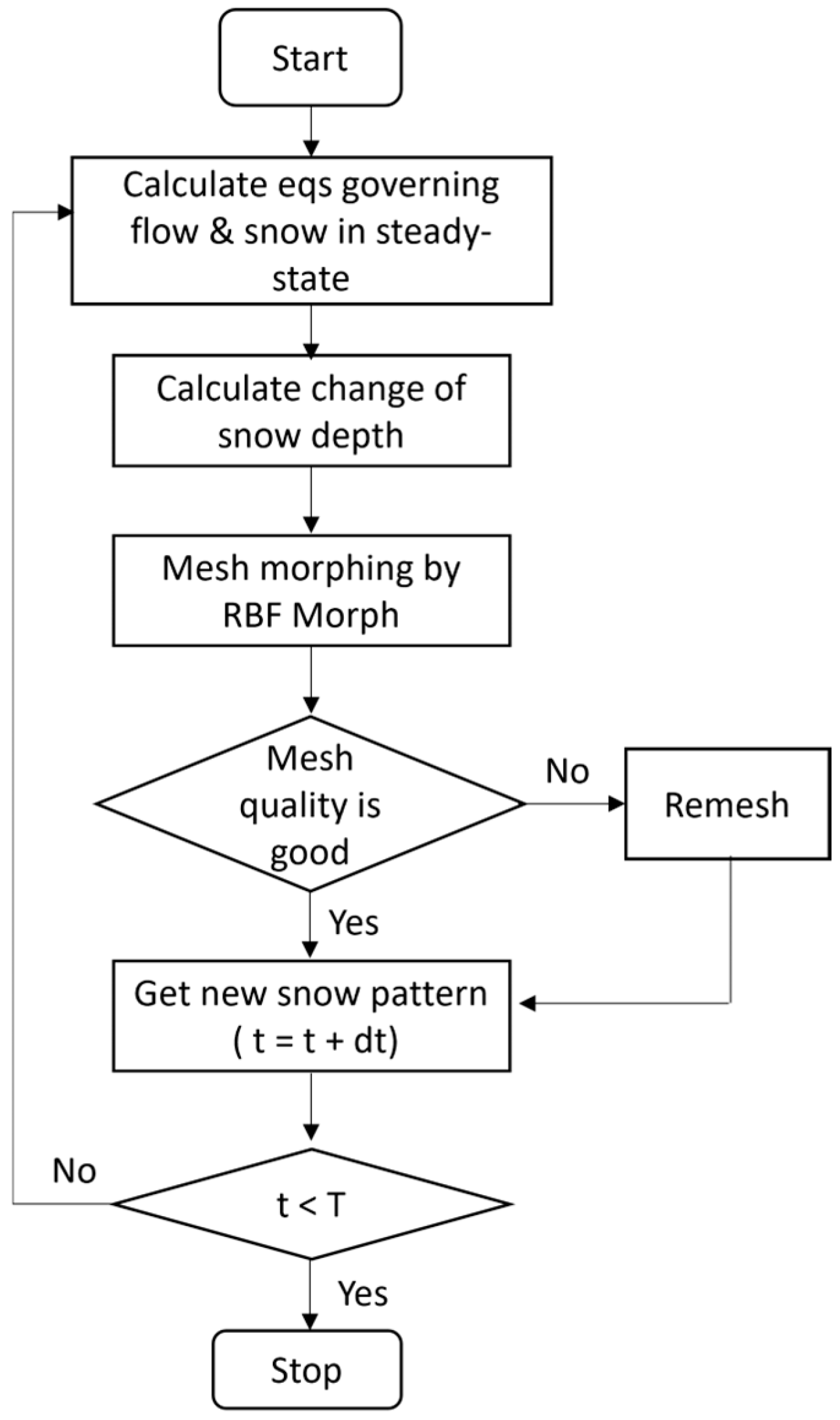
Figure 2 shows the calculation process of snow drifting based on the time-marching method using RBF interpolation.

2.5. Mesh-Morphing Method

The change in height of the cell vertices shown in Equation (21) is implemented on the wet surfaces and then extended to the other ones and to the volume elements of the computational grid using the RBF method. Displacements are applied along the geometry normal, prescribing a zero-motion field on the boundaries of fixed domains, obtaining a smooth displacement field in between. This approach can be obtained by exploiting one of the major characteristics of the RBF method, that is, its capability of performing a smooth interpolation of scalar information defined at points (source points), as a function of the distance [27]. The behavior of the interpolation between defined points depends on the kind of radial function employed, and the problem can be defined in an n-dimensional space by computing the distances between nodes as the Euclidean norm in the case of morphing [28]. By defining a deformation field of the mesh, the original grid topology is preserved during morphing [29,30]. To determine the system coefficients, a linear system of order equivalent to the number of utilized points [27] needs to be solved. Once these coefficients are obtained, the displacement of a specific node within the mesh can be calculated by superimposing the radial contributions from each source point. This applies to both interpolation (for nodes inside the domain) and extrapolation (for nodes outside the domain). The interpolation function is composed of a basis function $\varphi$ and a polynomial $h$ of the form $h\left(\mathrm{X}\right)={\beta }_1+{\beta }_2{x}_1+{\beta }_3{x}_2+\cdots +{\beta }_{n+1}{x}_n$. The degree of the polynomial term depends on the type of basis chosen. The inclusion of the polynomial term ensures problem uniqueness and polynomial precision, enabling the recovery of rigid body translations with accuracy. If N is the total number of source points, it can be written as follows:

$$s\left(\mathrm{X}\right)=\sum _{i=1}^N{\gamma }_i\varphi \left(‖\mathrm{X}-{\mathrm{X}}_{k_i}‖\right)+h\left(\mathrm{X}\right)$$

(22)

where $\mathrm{X}$ is the vector defining the coordinates at which the value is interpolated, and ${\mathrm{X}}_{k_i}$ is the i-th source point’s coordinate vector.

An interpolation exists if there are coefficients ${\gamma }_i$ for the RBF kernel and weights $\beta$ for the polynomial term, guaranteeing the exact value at source points during interpolation. In this case, the polynomial contribution should be zero. The RBF problem can be easily solved by resorting to matrix notation. In this case, the problem can be written as follows:

$$\left[\begin{array}{cc}M& P\\ P^{ᵀ}& 0\end{array}\right]\left\{\begin{array}{c}\gamma \\ \beta \end{array}\right\}=\left\{\begin{array}{c}g\\ 0\end{array}\right\}$$

(23)

where $g$ is the vector of known terms for each source point, and $M$ is the interpolation matrix with the radial distances between source points:

$$M_{ij}=\phi \left(\parallel x_{ki}-x_{kj}\parallel \right), 1\le i\le N, 1\le j\le N$$

(24)

$P$ is the constraint matrix containing the coordinates of source points in the space:

$$P=\left(\begin{array}{cccc}1& x_{k1}& y_{k1}& z_{k1}\\ 1& x_{k2}& y_{k2}& z_{k2}\\ ⋮& ⋮& ⋮& \\ 1& x_{kN}& y_{kN}& z_{kN}\end{array}\right)$$

(25)

Once the weights and coefficients of the system have been obtained, displacement values for the three directions can be easily obtained. For a three-dimensional case, in which the interpolated scalar is the mesh deformation, the following can be used to retrieve nodal displacements for a given point $\mathrm{X}$:

$$\left\{\begin{array}{c}{S}_x\left(\mathrm{x}\right)={\sum }_{i=1}^N{\gamma }_i^x\varphi (\Vert \mathrm{x}-{\mathrm{x}}_{k_i}\Vert )+{\beta }_1^x+{\beta }_2^x{x}_1+{\beta }_3^x{x}_2+{\beta }_4^x{x}_n\\ S_y\left(\mathrm{x}\right)={\sum }_{i=1}^N{\gamma }_i^y\varphi (\Vert \mathrm{x}-{\mathrm{x}}_{k_i}\Vert )+{\beta }_1^y+{\beta }_2^y{x}_1+{\beta }_3^y{x}_2+{\beta }_4^y{x}_n\\ S_z\left(\mathrm{x}\right)={\sum }_{i=1}^N{\gamma }_i^z\varphi (\Vert \mathrm{x}-{\mathrm{x}}_{k_i}\Vert )+{\beta }_1^z+{\beta }_2^z{x}_1+{\beta }_3^z{x}_2+{\beta }_4^z{x}_n\end{array}\right.$$

(26)

Thanks to its analytical nature, the RBF kernel can be differentiated by using the Kansa method, as shown in [31]. It is worth noting that the mesh size has been optimized, as usual, according to standard practice to ensure a mesh-independent solution, with the more stringent requirement of having a baseline mesh quality good enough to accept the morphing deformations without losing accuracy.

3. Results and Discussion

3.1. Cubic Building

3.1.1. Overview of the Cubic Building Problem

This study focused on the flow field and snow depth distribution around a cubic building with a side length of 1 m, as conducted by Oikawa et al. [32]. The experimental case SN19, characterized by low wind velocity and stable wind conditions, was selected for analysis. Okaze et al. [20] performed simulations on SN19, assuming a snowfall duration of 9 h to achieve a snow depth increase of 0.1 m over one day, and they provided the snow mass concentration corresponding to this snowfall condition. In this paper, we adopted the same snowfall conditions for the analysis.

The computational domain is shown in Figure 3a. Additionally, Figure 3b illustrates the mesh around the cubic building. The mesh was created using Ansys Fluent Meshing 2022R2 with the Poly-Hexcore method, and the total mesh count was 1.76 million cells.

Table 1. Parameters related to snow particles for the cubic building problem.

Threshold friction velocity	0.164 (m/s)
Aerodynamic roughness height	1.0 × 10−4 (m)
Density of snow particle	100.0 (kg/m3)
Diameter of snow particle	1.0 × 10−4 (m)
Falling velocity of snow particle $w_{f\_sky}$	1.0 (m/s)
Falling velocity of snow particle $w_{f\_surf}$	0.3 (m/s)

presents the parameters related to the physical properties of snow particles. The threshold friction velocity $u_{*t}$ was calculated using Equation (22) derived by Bagnold [33]. Ice density and air density were calculated as 917 kg/m³ and 1.332 kg/m³, respectively. The main analysis conditions for the flow field and the analysis conditions for the snow mass concentration equation are provided in

Table 2. Analysis conditions for the cubic building problem.

Inlet	$V_{in}=3.7z^{0.14}$ (m/s) Average wind direction is a 10-degree rotation from the normal direction to the front of the cubic building
	Snow mass concentration $\phi =1.913580214\times {10}^{-4}$ (kg/m3)
	Snow mass concentration ${\phi }_s=0.0$ (kg/m3)
	Inlet fetch distance $x_{in}^{\prime }=0$ (m)
	Reynolds number 2.93 × 105
Side	Symmetry
Top	Slip wall
	Zero gradient in normal direction
Outlet	0 (Pa)
	Zero gradient in normal direction
Building, ground	No slip wall, standard wall function
	$-{\displaystyle \frac{{\nu }_t}{{\sigma }_s}}\left({\displaystyle \frac{\partial \phi }{\partial x_j}}\right)=0$
	$-{\displaystyle \frac{{\nu }_t}{{\sigma }_s}}\left({\displaystyle \frac{\partial {\phi }_s}{\partial x_j}}\right)={\displaystyle \frac{\left|q_{eroshear}\right|+q_{slt}}{Area}}$
Turbulence model	Realizable $k-\epsilon$
Advection scheme	Momentum: QUICK
	Others: Second-Order Upwind
Time-marching step size	30 (min)

. The snow depth is dimensionless and normalized with respect to the reference snow depth of 0.1 m.

$$u_{*t}=A\sqrt{{\displaystyle \frac{{\rho }_i-{\rho }_f}{{\rho }_f}}gd}$$

(27)

where $A$ is the threshold parameter, and we adopted $A=0.2$ according to Clifton et al. [34].

3.1.2. Comparison of Observation and Analysis Results of the Cubic Building Problem

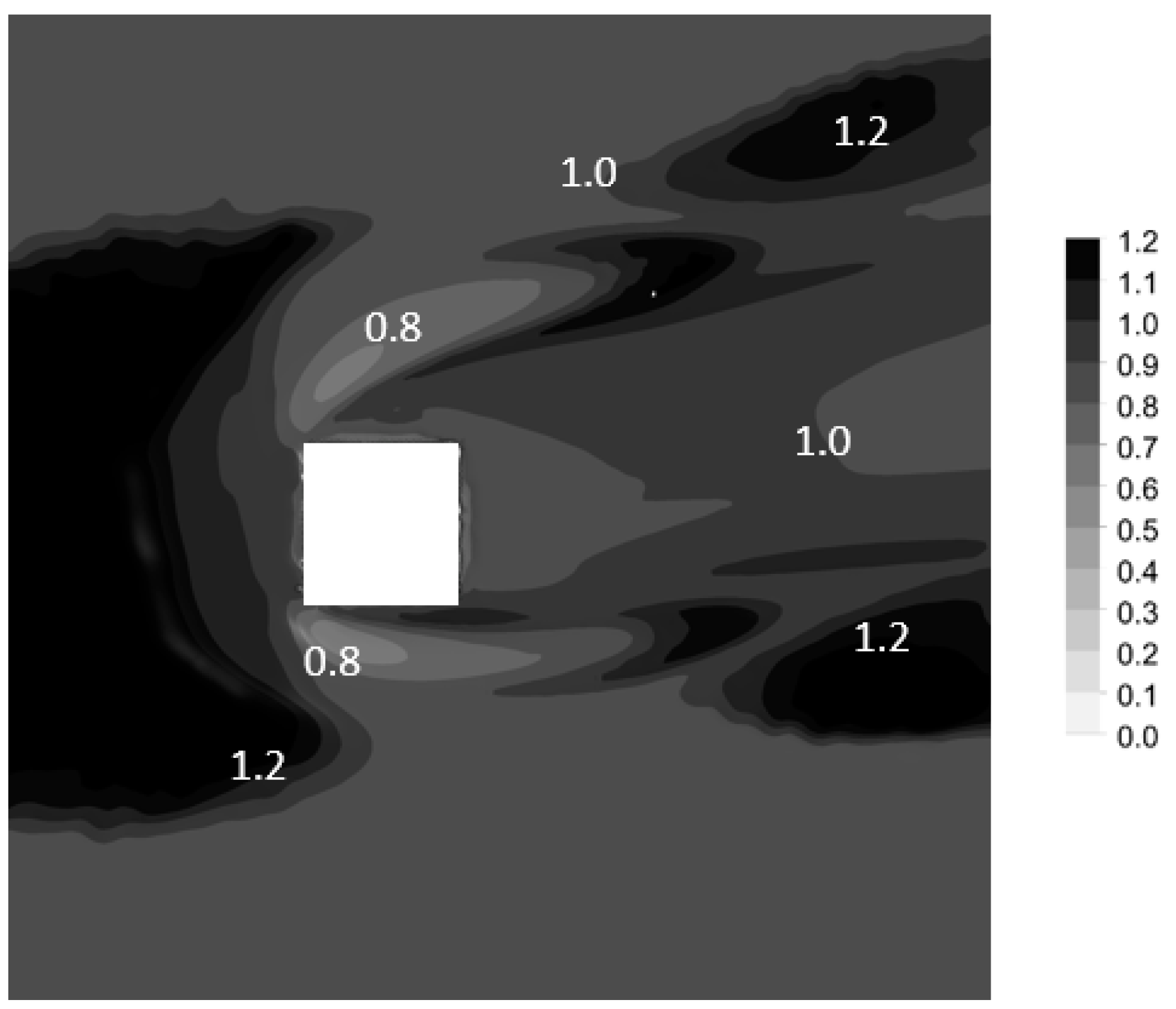
Figure 4a presents the observed snow depth distribution from Oikawa et al. [32], while Figure 4b shows the snow depth distribution obtained from the simulation results. In both cases, the snow depth decreases due to blowing snow in the detachment region on the side of the building, and overall quantitative agreement is achieved. Additionally, the formation of snowdrifts on the lee side is quantitatively captured in the results, indicating a good understanding of the trend. Figure 5 illustrates the snow depth distribution for the y/H = −1 cross-section and the x/H = 0 cross-section. The snow depth trend in the blowing region on the side of the building is captured, but the predicted snowdrift region is slightly displaced forward compared to the observed results. Furthermore, the reproduction of the snowdrift in front of the building is not achieved. The discrepancy between the analysis results and the observed snowdrifts in the stagnation region in front of the building can be attributed to the difference in wind speed characteristics. The analysis conditions were based on the average wind velocity over a 9 h snowfall period, while the observations revealed the presence of time intervals with higher wind velocity exceeding the average by approximately 1 m/s, as reported by Oikawa et al. [32]. The development of the saltation layer upstream and the occurrence of snowdrifts in the stagnation region are believed to be influenced by these periods of higher wind velocity. Since the analysis conditions did not accurately reproduce the specific wind velocity variations observed in Oikawa et al.’s data, the model failed to replicate the formation of snowdrifts in the stagnation region. Further refinement of the analysis conditions, taking into account the actual wind velocity variations observed during the measurements, may be necessary to improve the agreement between the analysis results and the observed snowdrift patterns.

In order to address the discrepancy and reproduce the formation of snowdrifts in the stagnation region, a new analysis was conducted. During the 9 h snowfall period, the first hour was set to a high-wind-velocity condition at a velocity of 4.5 m/s at a height of 1 m above ground level. Subsequently, for the remaining 8 h, the average wind velocity was set to 3.7 m/s, and for the last 8 h, it was adjusted to 3.6 m/s. By analyzing the high-wind-velocity condition, the aim was to investigate the occurrence of saltation and its influence on the formation of snowdrifts in front of the object. This approach was expected to provide a more accurate representation of the wind velocity variations observed in Oikawa et al. [32] and potentially lead to improved agreement between the simulation results and the observed snowdrift patterns.

In the observations conducted by Oikawa et al. [32], the cubic building was positioned on university campus grounds. Consequently, the development of the saltation layer from the campus grounds to the cubic building was expected to extend up to approximately 200 m. Therefore, in this study, the analysis was carried out assuming that the saltation layer started developing at a distance of 100 m upstream of the computational domain, and the inlet fetch distance was set to 100 m for the analysis. By considering the inlet fetch distance of 100 m, the analysis aimed to take into account the development of the saltation layer up to that point, which was expected to provide a more realistic representation of the conditions leading to snowdrift formation around the cubic building.

Figure 6 shows the snow depth distribution, while Figure 7 displays the snow depth distribution for the y/H = −1.0 cross-section and the x/H = 0 cross-section. Observing Figure 6, it can be seen that the snowdrift patterns on the lateral side of the cubic building and the accumulation on its lee side are consistent with the observed trends. Furthermore, the snowdrift in front of the cubic building is well reproduced, with its distribution extending over a wide area, similar to the observation results. Figure 7 also demonstrates that the snow depth distribution for the y/H = −1.0 cross-section, including the blowing snow on the building’s side and the accumulation on its lee side, is in good quantitative agreement with the observations. Moreover, the snowdrift in front of the object is successfully reproduced. The x/H = 0 cross-section also generally exhibits trends similar to the observation results. This suggests that the development of the saltation layer significantly impacts the snow depth distribution. The results indicate that the presence or absence of a developed saltation layer has a profound influence on the snowdrift patterns, highlighting the importance of considering saltation in the simulation of snow accumulation around the cubic building. In order to accurately assess snow depth, it is essential to consider more detailed field data regarding wind speed, wind direction, and saltation fetch distance. By incorporating such data into simulations, a more realistic representation of the conditions can be achieved, and it is anticipated that this would lead to an improvement in the overestimation of snow depth in front of the cubic building. Obtaining more precise field data, covering various wind conditions and terrain configurations, would enhance the reliability of the analyses and allow for more appropriate snowdrift analysis around buildings. Further research and data collection are crucial for deepening our understanding of this field.

3.2. Porous Fence

3.2.1. Overview of the Porous Fence Problem

Snow fences are structures designed to concentrate accumulated snow in specific areas, minimizing snow accumulation in other locations. They are commonly installed alongside highways to prevent snow from accumulating on the roads, thereby improving road visibility. In this study, we focused on the flow patterns around porous snow fences and the subsequent snowdrift phenomena, based on the measurements conducted by Tabler [35] and Iversen [36] around snow fences. Beyers [23] conducted a quantitative comparison with measurement results using a porous snow fence as the subject of analysis, and in this paper, we followed Beyers’ analysis conditions for our own simulations.

The analysis aims to understand the flow dynamics around snow fences and how they influence the formation of snowdrifts in their vicinity. By studying the interaction between the porous fences and the surrounding airflow, valuable insights can be gained for optimizing the design and placement of snow fences to effectively control snow accumulation and enhance winter road safety.

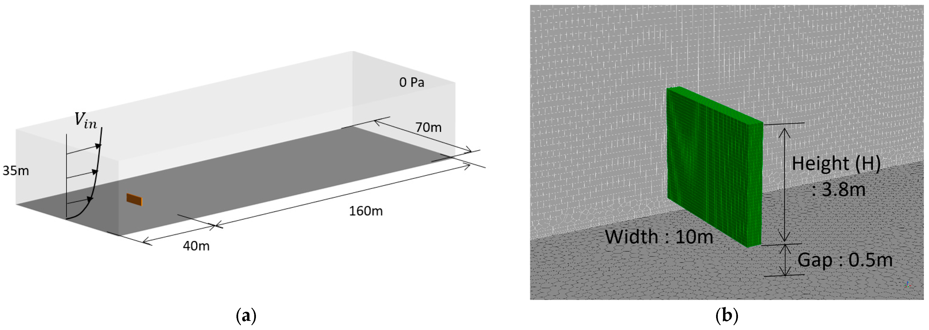
The computational domain and the mesh around the porous snow fence are shown in Figure 8, and the mesh was generated using Ansys Fluent Meshing 2022R2 with Poly-Hexcore, and the total mesh count was 1.96 million cells.

Table 3. Parameters related to snow particles for the porous fence problem.

Threshold friction velocity	0.28 (m/s)
Aerodynamic roughness height	1.0 × 10−4 (m)
Density of snow particle	150.0 (kg/m3)
Diameter of snow particle	1.1 × 10−4 (m)
Falling velocity of snow particle $w_{f\_sky}$	0.45 (m/s)
Falling velocity of snow particle $w_{f\_surf}$	0.3 (m/s)

presents parameters related to the physical properties of snow particles. The main analysis conditions for the flow field and the analysis conditions for the snow mass concentration equation are provided in

Table 4. Analysis conditions for the porous fence problem.

Inlet	$V_{in}=u_{*in}\left({\displaystyle \frac{1}{\kappa }}\mathit{ln}\left({\displaystyle \frac{z{u}_{*}}{\nu }}\right)+B-\Delta B(k_s^{+})\right)$ $u_{*in}=0.35,$ $B=5.5,$ $\Delta B\left(k_s^{+}\right)={\displaystyle \frac{1}{\kappa }}\left(1+0.3k_s^{+}+9.53s^{+}\right)$
	Snow mass concentration $\phi =1.0\times {10}^{-4}$ (kg/m3)
	Snow mass concentration ${\phi }_s={\displaystyle \frac{Q_{slt}\left(x^{\prime }\right)}{h_s{u}_p}}$ (kg/m3)
	Inlet fetch distance $x_{in}^{\prime }=300$ (m)
	Reynolds number 2.85 × 106
Side	Symmetry
Top	Slip wall
	Zero gradient in normal direction
Outlet	0 (Pa)
	Zero gradient in normal direction
Building, ground	No slip wall, standard wall function
	$-{\displaystyle \frac{{\nu }_t}{{\sigma }_s}}\left({\displaystyle \frac{\partial \phi }{\partial x_j}}\right)=0$
	$-{\displaystyle \frac{{\nu }_t}{{\sigma }_s}}\left({\displaystyle \frac{\partial {\phi }_s}{\partial x_j}}\right)={\displaystyle \frac{\left|q_{eroshear}\right|+q_{slt}}{Area}}$
Turbulence model	Realizable $k-\epsilon$
Advection scheme	Momentum: QUICK
	Others: Second-Order Upwind
Time-marching step size	30 (min)

. In this simulation, the inlet velocity $V_{in}$ was assumed to be greater than the threshold friction velocity, indicating the development of a saltation layer from the upstream region of the computational domain. The fetch distance for this assumption was set to 300 m. Additionally, the snow mass concentration at the inlet of the computational domain was determined using Equation (17), along with the mean saltating particle velocity $u_p$ and saltation height $h_s$. The mean saltating particle velocity $u_p$ is proportional to the threshold friction velocity, as shown by Pomeroy [37] and Pomeroy and Gray [6]:

$$u_p=c{u}_{*t}$$

(28)

with $c=2.3$, and this velocity remains constant during saltation. And the saltation height is defined as per Greeley and Iversen [38] as the ratio between the measured total snow transport and the mean snow mass flux, which is given by

$$h_s={\displaystyle \frac{1.6}{2g}}{u}_{*}^2$$

(29)

The momentum source due to the porous media is defined by the following equation:

$$S_i=-C_2{\displaystyle \frac{1}{2}}{\rho }_f\left|v_i\right|v_i$$

(30)

The parameter $C_2$ was set to 2.413, following the study by Byers [23].

3.2.2. Comparison of Observation and Analysis Results of the Porous Fence Problem

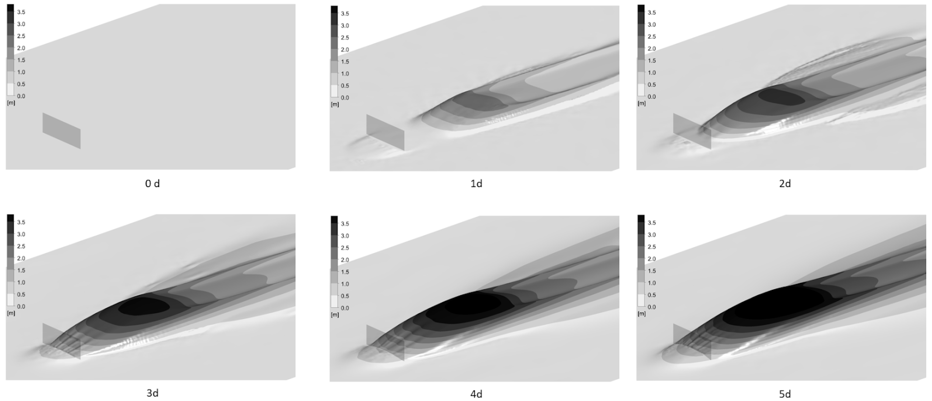
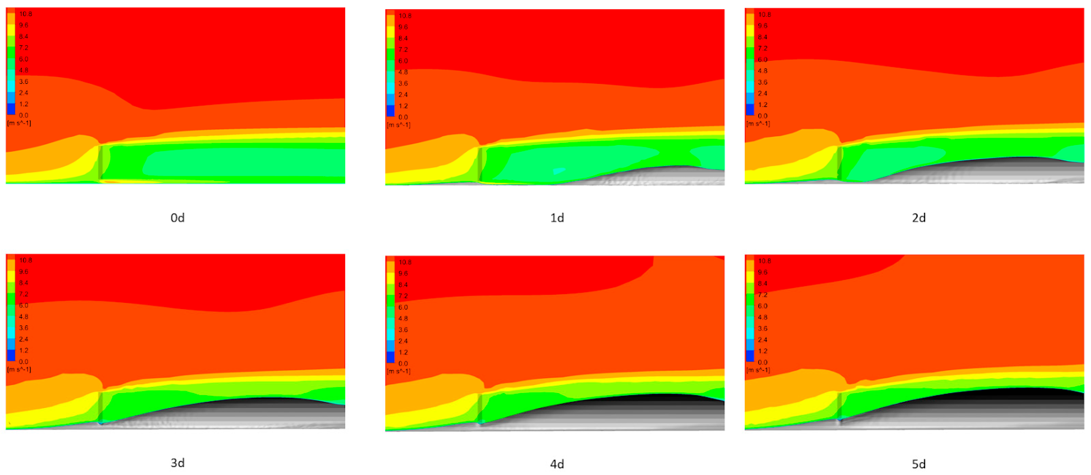
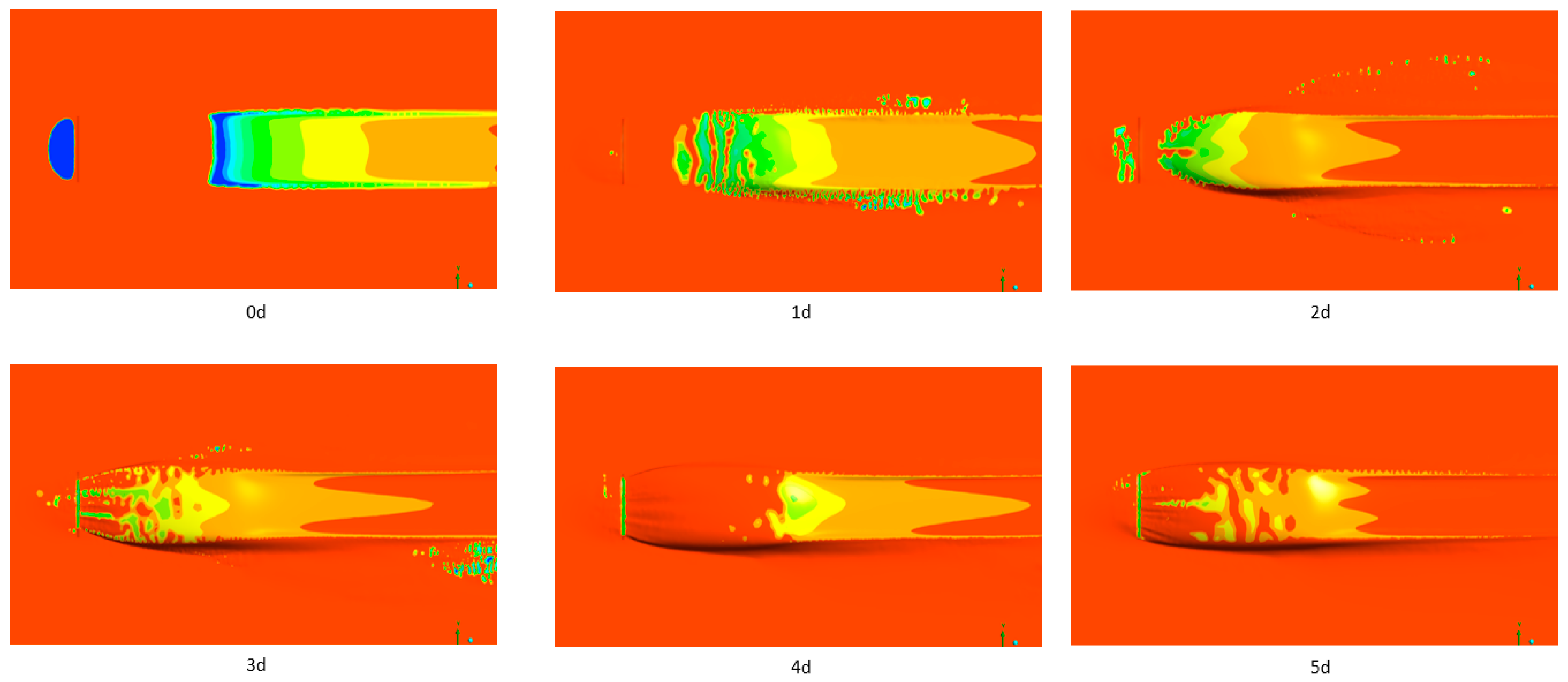
Figure 9 shows the snow depth contours, while Figure 10 shows the velocity contours. In the initial stage, it is observed that the flow is accelerated due to the presence of the porous snow fence and gaps on the snow surface, resulting in a blowing region. Downstream of this region, snowdrifts are formed. Additionally, upstream of the porous snow fence, where the flow decelerates, a weak snowdrift is formed. It is evident that this snowdrift undergoes changes in snow depth over time, gradually filling the gaps between the snow fence and the snow surface. As the gaps become smaller, the velocity decreases, leading to a gradual reduction in the blowing region downstream of the snow fence. Consequently, the snowdrift region downstream of the snow fence tends to extend upstream over time. Figure 11a shows the drifted snow profile on the xz plane at y = 0.0 m. The drifted snow profile from the snow fence to the snowdrift peak position closely matches the results of the snowdrift measurements conducted by Tabler [35] and Iversen [36]. However, it is evident that the snow depth is underestimated from the snowdrift peak position to x/H = 20. Moreover, the significant negative gradient of snow depth from the snowdrift peak position to x/H = 10, as indicated in the results, is not observed in the actual measurements. Figure 11b presents the temporal variation in snow depth at y = 0 and in Figure 12 the relative contours. Upon examining the change in snow depth, it is evident that initially, the snow depth transitions with a gentle negative gradient from the peak position, and this gradient increases over time. According to Equation (17), the saltation transport rate $Q_{slt}\left(x^{\prime }\right)$ within the saltation layer is a function of the saltation fetch distance, and the distribution of snow depth at snowdrift locations can vary depending on its value. In this analysis, we assumed that the snow fence was installed in an open and wide space based on data from Beyers [23], setting the saltation fetch distance to 300 m. However, it is expected that the saltation transport rate will significantly change, and consequently, the snow depth distribution will be affected by the choice of this value. Determining the appropriate value for the saltation fetch distance requires more detailed data, such as the degree of saltation development. To understand the cause of the underestimation of snow depth, a more in-depth investigation is necessary for further research and efforts.

3.3. Two-Level Flat Roof

3.3.1. Overview of the Two-Level Flat Room Problem

When observing snow accumulation on building rooftops, in the case of a simple flat roof, the snow imbalance on the rooftop is relatively small, making it less problematic when evaluating snow loads. But in the case of roofs with stepped setbacks, it is known that snowdrifts can form on the lower sections of the roof. In this paper, we focused on a model simulating a building with a stepped roof shape and conducted a comparison with the field observation results of Tsuchiya et al. [39].

The computational domain and the mesh around the porous snow fence are shown in Figure 13, and the mesh was generated using Ansys Fluent Meshing 2022R2 with Poly-Hexcore, and the total mesh count was 779,000 cells.

Table 5. Parameters related to snow particles for the two-level flat room problem.

Threshold friction velocity	0.20 (m/s)
Aerodynamic roughness height	2.0 × 10−3 (m)
Density of snow particle	250.0 (kg/m3)
Diameter of snow particle	1.1 × 10−4 (m)
Falling velocity of snow particle $w_{f\_sky}$	0.20 (m/s)
Falling velocity of snow particle $w_{f\_surf}$	0.20 (m/s)

presents parameters related to the physical properties of snow particles. The main analysis conditions for the flow field and the analysis conditions for the snow mass concentration equation are provided in

Table 6. Analysis conditions for the two-level flat room problem.

Inlet	$V_{in}={\displaystyle \frac{u_{*in}}{\kappa }}\mathit{ln}\left({\displaystyle \frac{z}{z_0}}+1\right)$ $u_{*in}=1.0, z_0=0.002, \kappa$ is the Karman constant
	Snow mass concentration $\phi =0$ (kg/m3)
	Snow mass concentration ${\phi }_s=0$ (kg/m3)
	Inlet fetch distance $x_{in}^{\prime }=0$ (m)
	Reynolds number 2.25 × 106
Side	Symmetry
Top	Slip wall
	Zero gradient in normal direction
Outlet	0 (Pa)
	Zero gradient in normal direction
Building, ground	No slip wall, standard wall function
	$-{\displaystyle \frac{{\nu }_t}{{\sigma }_s}}\left({\displaystyle \frac{\partial \phi }{\partial x_j}}\right)=0$
	$-{\displaystyle \frac{{\nu }_t}{{\sigma }_s}}\left({\displaystyle \frac{\partial {\phi }_s}{\partial x_j}}\right)={\displaystyle \frac{\left|q_{eroshear}\right|+q_{slt}}{Area}}$
Turbulence model	Realizable $k-\epsilon$
Advection scheme	Momentum: QUICK
	Others: Second-Order Upwind
Time-marching step size	120 (min)

. In this simulation, to disregard the effects of changes in snow depth around the two-level flat roof, alterations in the snow surface on the ground were not considered. Additionally, snowfall was assumed to be absent.

In order to approximate the real snow drifting phenomenon to some extent, the characteristic length was set to H = 3.0 m. The initial snow depth was 0.5 m on the lower roof. These values were determined with reference to the analysis conditions of Zhu et al. [14].

3.3.2. Comparison of Observation and Analysis Results of the Two-Level Flat Room Problem

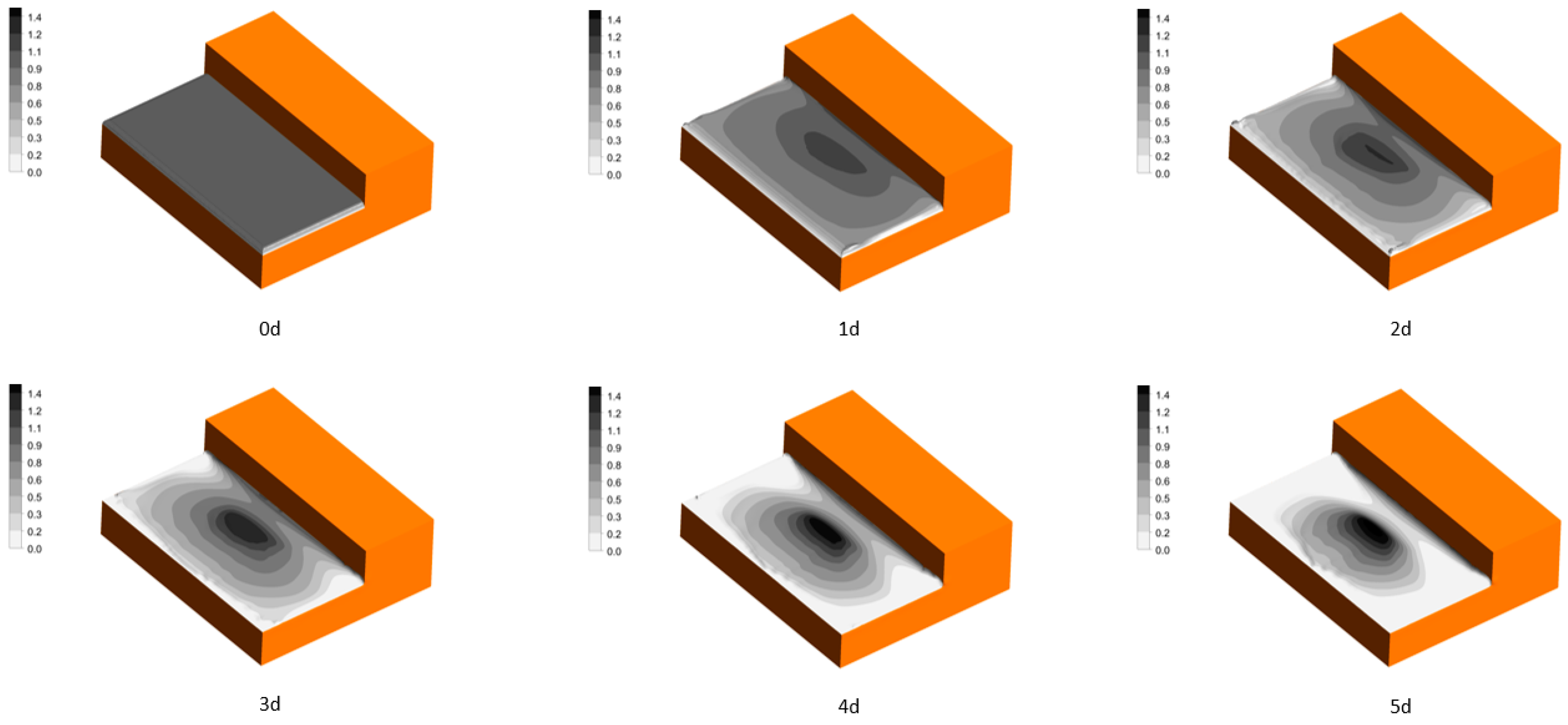
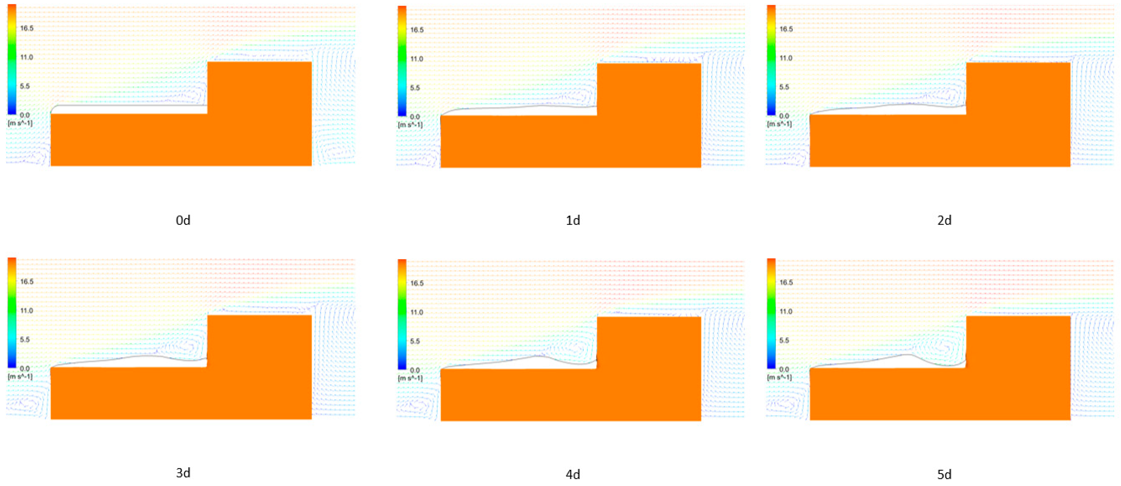
Figure 14 shows the distribution of snow depth normalized by the initial snow depth of 0.5 m on the lower roof, while Figure 15 displays the velocity vectors at the cross-section passing through the center of the two-level flat roof, y/H = 0. At the initial stage of the analysis, it is evident that strong flow separation occurs at the lower end of the stepped roof. As a result, the snow surface near the lower end experiences erosion due to the strong shear forces, leading to a decrease in snow depth from the end. On the other hand, in the central area of the lower section of the roof, the formation of a snowdrift can be observed. This is believed to have resulted from the erosion of the snow surface upstream of the snowdrift, where snow particles were lifted from the surface and deposited, leading to the accumulation of snow and the formation of the snowdrift, as indicated in Figure 16a,b. At the stepped section, flow separation vortices indeed occur, and as time progresses, it becomes evident that the developing snowdrift causes even stronger flow separation vortices to form. These flow separation vortices lead to the erosion of the snow surface at the stepped section. Figure 17a depicts the snow depth distribution on the lower section of the roof at y/H = 0, compared with the field observation results of Tsuchiya et al. [39]. The simulation results accurately capture the trend of the monotonically increasing snow depth distribution from x/H = 0 to x/H = 1.5, just like the field observations. It is evident that the snow depth peaks around x/H = 1.8, slightly upwind compared to the field observations. However, around x/H = 2.7, erosion due to vortices occurs, and the peak position and snow depth are well captured quantitatively as well as qualitatively. Figure 17b represents the 5-day variation in the snow distribution on the lower section of the roof at y/H = 0. From x/H = 0 to x/H = 1, it can be observed that there is significant erosion of the snow surface at the initial stage of the calculations. As a consequence of this erosion, snow particles are lifted and accumulate, leading to the formation of snowdrifts. Additionally, around x/H = 2.7, flow separation vortices have developed, accelerating the erosion at the stepped section due to their influence.

4. Conclusions

• In this study, we conducted a numerical simulation of snowdrifts considering the fetch distance of the saltation layer to predict drifting snow phenomena around buildings. We performed a snowdrift analysis to quantitatively compare the simulation results with actual measurements of snow depth near the buildings;
• In the case of studying drifting snow phenomena around cubic buildings, it was observed that without the development of a saltation layer under the average wind velocity, the snowdrifts in front of the cube were not reproduced accurately in the simulation. However, when considering the conditions for the development of a saltation layer, the snowdrifts were successfully reproduced, leading to relatively good agreement between the simulation results and actual measurements;
• In the snow porous fence, the measured snow profile matches previous studies up to the snowdrift peak position but underestimates the snow depth beyond that point. The snow depth initially decreases gently from the peak position and then increases over time. The saltation transport rate $Q_{slt}\left(x^{\prime }\right)$ can change the snow depth distribution at the blowdown location. Therefore, the value of the saltation transport rate can vary greatly depending on the value of the saltation fetch distance, but more detailed data such as the degree of saltation development are considered necessary to determine its value;
• In the case of studying drifting snow phenomena around a two-level flat roof, the snow particles lifted by the erosion of the snow surface at the lower end of the stepped roof during the initial calculations contributed to the formation of snowdrifts downstream. As the snowdrifts formed, flow separation vortices developed downstream, which further accelerated the erosion. Overall, the distribution of snow depth showed relatively good qualitative and quantitative agreement between the simulation and actual measurements.

References

1. Mitsuhashi, H. Snowdrifting on building and wind tunnel experiment using model snow. J. Jpn. Soc. Snow Ice 2003, 65, 287–295. [Google Scholar]
2. Shuji, S.; Osamu, A.B.E.; Osamu, J.O.H. Wind Tunnel on effect of roof wind pressure of buildings on shaping roof snow accumulations. J. Struct. Constr. Eng. 2009, 74, 451–458. [Google Scholar]
3. Oikawa, S.; Tomabechi, T.; Ishihara, T. Study of wind tunnel similarity on snowdrift around buildings. Nagare 2007, 26, 319–324. [Google Scholar]
4. Uematsu, T.; Nakata, T.; Takeuchi, K.; Arisawa, Y.; Kaneda, Y. Three-dimensional numerical simulation of snowdrift. Cold Reg. Sci. Technol. 1991, 20, 65–73. [Google Scholar]
5. Iversen, J.D.; Greeley, R.; White, B.R.; Pollack, J.B. Eolian erosion of the Martian surface, part 1: Erosion rate similitude. Icarus 1980, 26, 321–331. [Google Scholar]
6. Pomeroy, J.W.; Gray, D.M. Saltation of snow. Water Resour. Res. 1990, 26, 1583–1594. [Google Scholar]
7. Okaze, T.; Mochida, A.; Yoshino, H.; Tominaga, Y.; Nemoto, M.; Sato, T.; Ito, Y. Modeling of snowdrift in non-equilibrium flowfields around buildings—(Part2) Universal relation between the streamwise distance and the transport rate of drifting snow. In Summaries of JSSI and JSSE Joint Conference on Snow and Ice Research; The Japanese Society of Snow and Ice/Japan Society for Snow Engineering: Tokyo, Japan, 2008; Volume 2008, p. 217. [Google Scholar]
8. Liston, G.E.; Sturm, M. A snow-transport model for complex terrain. J. Glaciol. 1998, 44, 498–516. [Google Scholar]
9. ANSYS Fluent; 2022R2; ANSYS Fluent Theory Guide; ANSYS Inc.: Canonsburg, PA, USA, 2022.
10. Beyers, M.; Waechter, B. Modeling transient snowdrift development around complex three-dimensional structures. J. Wind Eng. Ind. Aerodyn. 2008, 96, 1603–1615. [Google Scholar]
11. Thiis, T.; Ferreira, A.D. Sheltering effect and snow deposition in arrays of vertical pillars. Environ. Fluid Mech. 2015, 15, 27–39. [Google Scholar]
12. Zhou, X.; Kang, L.; Gu, M.; Qiu, L.; Hu, J. Numerical simulation and wind tunnel test for redistribution of snow on a flat roof. J. Wind Eng. Ind. Aerodyn. 2016, 153, 92–105. [Google Scholar]
13. Franke, R. Scattered data interpolation: Tests of some methods. Math. Comput. 1982, 38, 181–200. [Google Scholar]
14. Zhu, F.; Yu, Z.; Zhao, L.; Xue, M.; Zhao, S. Adaptive-mesh method using RBF interpolation: A time-marching analysis of steady snow drifting on stepped flat roofs. J. Wind Eng. Ind. Aerodyn. 2017, 171, 1–11. [Google Scholar] [CrossRef]
15. Groth, C.; Costa, E.; Biancolini, M.E. RBF-based mesh morphing approach to perform icing simulations in the aviation sector. Aircr. Eng. Aerosp. Technol. 2019, 91, 620–633. [Google Scholar] [CrossRef]
16. Mochida, A.; Yoshino, H.; Okaze, T.; Tominaga, Y.; Lto, Y. Modeling of snowdrift in non-equilibrium flowfields around buildings—(Part 3) New snowdrift model incorporating the effects of drifting snow particles on turbulent flow. In Summaries of JSSI and JSSE Joint Conference on Snow and Ice Research; The Japanese Society of Snow and Ice/Japan Society for Snow Engineering: Tokyo, Japan, 2008; Volume 2008, p. 218. [Google Scholar]
17. Lto, Y.; Tominage, Y.; Okaze, T.; Mochida, A.; Nemoto, M. Modeling of snowdrift in non-equilibrium flowfields around buildings–(Part1) Wind tunnel measurements of spatial distribution of mass flux of drifting snow in developing snow boundary layer. In Summaries of JSSI and JSSE Joint Conference on Snow and Ice Research; The Japanese Society of Snow and Ice/Japan Society for Snow Engineering: Tokyo, Japan, 2008; Volume 2008, p. 216. [Google Scholar]
18. Naaim, M.; Naaim-Bouvet, F.; Martinez, H. Numerical simulation of drifting snow: Erosion and deposition models. Ann. Glaciol. 1998, 26, 191–196. [Google Scholar] [CrossRef]
19. Launder, B.E.; Spalding, D.B. The numerical computation of turbulent flows. Comput. Methods Appl. Mech. Eng. 1974, 3, 269–289. [Google Scholar] [CrossRef]
20. Okaze, T.; Tominaga, Y.; Mochida, A. Development of new snowdrift model based on two transport equations of drifting snow density: Numerical prediction of snowdrift around buildings using CFD (Part 2). J. Environ. Eng. 2013, 78, 149–156. [Google Scholar] [CrossRef]
21. Sato, T.; Mochizuki, S.; Kosugi, K.; Nemoto, M. Effects of particle shape on mass flux measurement of drifting snow by snow particle counter. J. Jpn. Soc. Snow Ice 2005, 67, 493–503. [Google Scholar] [CrossRef]
22. Moore, I. Numerical Modeling of Blowing Snow Around Buildings. Ph.D. Thesis, Department of Applied Mathematical Studies, University of Leeds, Leeds, UK, 1995. [Google Scholar]
23. Beyers, J.H.M. Numerical Modeling of the Snow Flow Characteristics Surrounding SANAE IV Research Station, Antarctica. Ph.D. Thesis, Department of Mechanical Engineering, University of Stellenbosch, Stellenbosch, South Africa, 2004. [Google Scholar]
24. Nemoto, M.; Nishimura, K.; Kobayashi, S.; Izumi, K. Numerical study of the time development of drifting snow and its relation to the spatial development. Ann. Glaciol. 2004, 38, 343–350. [Google Scholar] [CrossRef]
25. Xu, Y.; Xu, Y.; Mustafa, M.Y.; Mustafa, M.Y.; Solvang, W.D.; Solvang, W.D. CFD aided cognitive capabilities for analyzing snowdrift development around a porous fence. In Proceedings of the 2014 5th IEEE Conference on Cognitive Infocommunications (CogInfoCom), Vietri sul Mare, Italy, 5–7 November 2014. [Google Scholar]
26. Shao, Y.; Li, A. Numerical modeling of saltation in the atmospheric surface layer. Bound.-Layer Meteorol. 1999, 91, 199–225. [Google Scholar] [CrossRef]
27. Buhmann, M.D. Radial basis functions. Acta Numer. 2000, 9, 1–38. [Google Scholar] [CrossRef]
28. de Boer, A.; van der Schoot, M.S.; Bijl, H. Mesh deformation based on radial basis function interpolation. Comput. Struct. 2007, 85, 784–795. [Google Scholar] [CrossRef]
29. Beckert, A.; Wendland, H. Multivariate interpolation for fluid-structure-interaction problems using radial basis functions. Aerosp. Sci. Technol. 2001, 2, 125–134. [Google Scholar] [CrossRef]
30. Biancolini, M.E. Fast Radial Basis Functions for Engineering Applications; Springer: Berlin/Heidelberg, Germany, 2018. [Google Scholar]
31. Chiappa, A.; Groth, C.; Biancolini, M.E. A two-scale RBF meshless method for the interface stress retrieval in simply bended and torqued long-fibres laminates. Compos. Struct. 2023, 306, 116600. [Google Scholar] [CrossRef]
32. Oikawa, S.; Tomabechi, T.; Ishihara, T. One-day observations of snowdrifts around a model cube. J. Snow Eng. Jpn. 1999, 15, 3–11. [Google Scholar] [CrossRef]
33. Bagnold, R.A. The Physics of Blown Sand and Desert Dunes; Methuen and Co.: London, UK, 1941. [Google Scholar]
34. Clifton, A.; Rüedi, J.-D.; Lehning, M. Snow saltation threshold measurements in a drifting-snow wind tunnel. J. Glaciol. 2006, 52, 585–596. [Google Scholar] [CrossRef]
35. Tabler, R.D. Geometry and density of drift formed by snow fences. J. Glaciol. 1980, 26, 405–419. [Google Scholar] [CrossRef]
36. Iversen, J.D. Comparison of wind tunnel model and full scale snow fence drifts. J. Wind Eng. Ind. Aerodyn. 1981, 8, 231–249. [Google Scholar] [CrossRef]
37. Pomeroy, J.W. A process-based model of snow drifting. Ann. Glaciol. 1989, 13, 237–240. [Google Scholar] [CrossRef]
38. Greeley, R.; Iversen, J.D. Wind as a Geological Process on Earth, Mars, Venus and Titan; Cambridge University Press: Cambridge, UK, 1985. [Google Scholar]
39. Tsuchiya, M.; Tomabechi, T.; Hongo, T.; Ueda, H. Characteristics of wind flow acting on snowdrift on a stepped flat roof. J. Struct. Constr. Eng. AIJ 2002, 67, 53–59. [Google Scholar] [CrossRef]
Figure 1. Control volume with the near-surface snow mass conservation.
Fluids 10 00075 g001
Figure 2. Flow chart of calculation.
Fluids 10 00075 g002
Figure 3. (a) Computational domain; (b) mesh around the cubic building.
Fluids 10 00075 g003
Figure 4. Snow depth patterns which are made dimensionless with the reference snow depth of 0.1 (m): (a) field observations by Oikawa et al. [32]; (b) simulation results.
Fluids 10 00075 g004
Figure 5. Comparison of snow depth between field observation results and numerical simulation results computed considering a constant wind speed: (a) cross-section passing through the center of the building, x/H = 0.0 [32]; (b) streamwise section near the building, y/H = −1.0 [32].
Fluids 10 00075 g005
Figure 6. Snow depth patterns which are made dimensionless with the reference snow depth of 0.1 (m).
Fluids 10 00075 g006
Figure 7. Comparison of snow depth between field observation results and numerical simulation results computed considering variable wind speed: (a) cross-section passing through the center of the building, x/H = 0.0 [32]; (b) streamwise section near the building, y/H = −1.0 [32].
Fluids 10 00075 g007
Figure 8. (a) Computational domain; (b) mesh around the porous fence.
Fluids 10 00075 g008
Figure 9. Five-day variation in snow depth patterns around the porous snow fence.
Fluids 10 00075 g009
Figure 10. Five-day variation in velocity contour around the porous snow fence.
Fluids 10 00075 g010
Figure 11. Snow depth normalized by snow fence height H = 3.8 m at cross-section passing through the center of the porous fence, y/H = 0: (a) comparison of snow depth between field observation results and numerical simulation results [35,36]; (b) 5-day variation in snow depth patterns.
Fluids 10 00075 g011
Figure 12. Five-day variation in saltation deposit flux contour on snow surface.
Fluids 10 00075 g012
Figure 13. (a) Computational domain; (b) mesh around the two-level flat roof.
Fluids 10 00075 g013
Figure 14. Five-day variation in snow depth patterns on the lower roof.
Fluids 10 00075 g014
Figure 15. Five-day variation in velocity vectors around the two-level flat roof.
Fluids 10 00075 g015
Figure 16. (a) Erosive flux contour; (b) saltation deposit flux contour.
Fluids 10 00075 g016
Figure 17. Snow depth normalized by the initial snow depth of 0.5 m at the cross-section passing through the center of the two-level flat roof, y/H = 0: (a) comparison of snow depth between field observation results and numerical simulation results [39]; (b) 5-day variation in snow depth patterns.
Fluids 10 00075 g017