Abstract
Understanding the rheological properties of fresh cement slurries is essential to maintain optimal pumpability, achieve dependable zonal isolation, and preserve long-term well integrity in oil and gas cementing operations and the 3D printing cement and concrete industry. However, accurately and efficiently modeling the rheological behavior of cement slurries remains challenging due to the complex fluid properties of fresh cement slurries, which exhibit non-Newtonian and thixotropic behavior. Traditional numerical solvers typically require mesh generation and intensive computation, making them less practical for data-scarce, high-dimensional problems. In this study, a physics-informed neural network (PINN)-based framework is developed to solve the governing equations of steady-state cement slurry flow in a tilted channel. The slurry is modeled as a non-Newtonian fluid with viscosity dependent on both the shear rate and particle volume fraction. The PINN-based approach incorporates physical laws into the loss function, offering mesh-free solutions with strong generalization ability. The results show that PINNs accurately capture the trend of velocity and volume fraction profiles under varying material and flow parameters. Compared to conventional solvers, the PINN solution offers a more efficient and flexible alternative for modeling complex rheological behavior in data-limited scenarios. These findings demonstrate the potential of PINNs as a robust tool for cement slurry rheological modeling, particularly in scenarios where traditional solvers are impractical. Future work will focus on enhancing model precision through hybrid learning strategies that incorporate labeled data, potentially enabling real-time predictive modeling for field applications.
1. Introduction
The rheological modeling of cement slurries is critical for ensuring effective placement and long-term durability in the cement and petroleum industries [1,2]. Computational models help predict parameters such as shear stress, viscosity, and yield point under varying temperatures, pressures, and additive compositions, which are essential for optimizing pumpability and zonal isolation, as shown in our previous work [1,2,3,4,5,6,7]. Cement slurries typically behave as complex, non-Newtonian thixotropic fluids whose nonlinear, stress-dependent characteristics are revealed through detailed stress analysis [8]. Their behavior is described using empirical models, including the power law model at high shear rates and the Bingham plastic model [9]. The power law model is useful for describing the behavior of various fluids, including cement slurries, despite its limitations at extreme shear rates. Several more realistic models with two parameters are used to describe the rheological properties of cement slurries, including the Casson (1959) [10], Vocadlo [11], and Herschel–Bulkley [12] models. The three-parameter Bingham plastic model can be more flexible under certain situations compared with two-parameter models. However, the third parameter (often empirical) in three-parameter models may not always correspond to a clear physical mechanism, making interpretation and generalization difficult. Laboratory measurements using pressurized viscometers and rheometers are conducted to obtain rheological parameters (plastic viscosity, yield point, and gel strength) at various temperatures and pressures [7,8]. These data are then used to parameterize the empirical models for simulation. Simulation methods for cement slurry rheology modeling typically involve a combination of experimental measurements, empirical models, and advanced computational techniques to predict and analyze slurry behavior under various conditions. Simulations for cement slurry rheology study have been conducted in previous studies, including steady flow [3], Poiseuille flow [4], and particle effects [6]. Despite significant advances in empirical and computational modeling, there remains a notable shortage in simulation accuracy and predictive power for cement slurry rheology, especially under complex, real-world conditions such as high pressure, high temperature, and variable additive compositions [3,7]. Empirical models often fail to fully capture the dynamic and nonlinear behavior of cement slurries, particularly when faced with extreme environmental changes or the presence of multiple additives [13,14]. Laboratory measurements provide essential data, but translating these into robust simulations for field-scale applications remains challenging due to the complexity of slurry behavior and the limitations of existing constitutive models [2].
Machine learning approaches offer promising potential to address these gaps. By leveraging large datasets from laboratory and field experiments, machine learning algorithms, such as artificial neural networks (ANNs), can learn complex relationships between slurry composition, environmental conditions, and rheological properties [15]. Early investigations into the use of neural networks for solving differential equations were conducted in the late 20th century, highlighting the longstanding interest in data-driven approaches to numerical analysis. Dissanayake et al. [16] transformed the solution of partial differential equations into an unconstrained minimization problem and used neural networks to solve a linear Poisson equation and a nonlinear thermal conduction equation. Lagaris et al. [17] used ANNs to fit the solution of PDEs with complex boundary conditions. Aarts et al. [18] combined single-hidden-layer feedforward networks to represent different-order differential operators and trained them together to solve partial differential equations. However, those machine learning methods were mainly based on data-driven methods, that is, obtaining exact solutions to partial differential equations in advance (often called “labeled data”), which caused great limitations because the analytic solution was usually hard to obtain. With the development of deep learning approaches and environments such as TensorFlow 1.10 and PyTorch1.0, researchers have started to make progress in solving complex physical and mathematical problems. The most groundbreaking work in this field was the PINN approach proposed by Raissi [19]. Physics-informed neural networks (PINNs) represent a powerful fusion of machine learning and classical physics-based modeling, designed to tackle complex ordinary and partial differential equations (ODEs and PDEs) that govern systems in fluid mechanics and civil engineering [16,17]. By embedding the governing equations directly into the loss function of a neural network, PINNs enforce physical laws during training, ensuring that the network’s predictions are consistent with fundamental conservation principles such as mass and momentum [20,21]. This approach allows PINNs to learn from both sparse and noisy experimental data while providing continuous solutions across the domain, even in scenarios where high-resolution reference data are unavailable. The solution of PDEs was approximated by inputting physical information into the neural network. The entire solution process only required control equations and boundary condition forms that could reflect physical information and did not require the “labeled data” mentioned above.
Based on the ideas of PINNs, researchers have proposed new methods of neural networks. Bandai et al. [22] used a PINN framework composed of three DNNs to perform parameter inversion of the Richardson–Richards equation and estimated the water retention curve and hydraulic conduction function. Han et al. [23] introduced a neural network method, the Derivative-Free Loss Method. When computing the training loss, this method did not require the explicit calculation of the derivatives of the neural network to the input neurons. It has been proved to be a powerful tool for solving elliptic PDEs. Almajid et al. [24] implied that though PINN could effectively capture the general pattern of the solution for PDEs, the precision and reliability of the solution would significantly increase when some labeled data were considered as a part of the loss function. Meanwhile, Cuomo [25] summarized variants of PINN, such as physics-constrained neural networks, variational hp-adaptive Variational PINN, and conservative PINN. Meng et al. [26] proposed an improved PINN method, Parareal PINN, which decomposed a long-term problem into multiple independent short-time problems to speed up the solution of partial differential equations.
While current PINN methodologies could offer a feasible solution to relatively straightforward problems, they often fail to combine with physical phenomena when confronted with some complex engineering problems. Thus, Krishnapriyan et al. [27] proposed two approaches, called curriculum regularization and sequence-to-sequence learning. The results demonstrated that the proposed methods could achieve lower error by up to 1–2 orders of magnitude compared to simple PINN. Furthermore, when faced with multi-scale, chaotic, or turbulent problems, Wang et al. [28] proposed a process to re-formulate the loss functions of PINN using a self-defined hyper-parameter that determines the “slope” of weights of loss functions. It shows superiority in addressing complex PDEs. Lawal et al. [29] collected abundant articles on computational sciences and engineering and proposed the three most promising development directions for PINN, which were extended PINN, hybrid PINN, and the minimization of its loss function.
In recent years, with the growth of data and the development of computation methods, PINN methods have been studied in fluid mechanics, offering possibilities to explore new solutions [30,31]. Lu et al. [32] proposed a new paradigm using PINN methods to understand the shear migration of particles in viscous flow. It demonstrates that PINNs significantly broaden the practical utility and adaptability of traditional phenomenological models by solving forward and inverse problems concurrently. Zhang et al. [33] introduced a PINN-based framework to embed complex PDEs into a well-designed architecture, linking macroscopic viscous flow behaviors and microstructural changes. It shows the great superiority of PINNs in analyzing rheological and thixotropic problems with accumulating computational costs needed in simulating numerous parameters in equations.
Despite these advances, applications of PINNs to non-Newtonian cement slurry flow remain unexplored. Key challenges include formulating a PINN that simultaneously solves momentum and continuity equations with appropriate rheological constitutive laws, balancing physics-based and data-driven loss components to avoid over- or under-fitting, and reducing computational cost while maintaining accuracy under high-pressure–high-temperature and multi-additive conditions. To address these gaps, this paper makes the following contributions: (1) A boundary-value problem for the steady, laminar flow of cement slurry between two tilted plates is formulated, incorporating temperature- and pressure-dependent rheological parameters. (2) A customized PINN architecture is designed, integrating the coupled momentum and continuity equations, rheological constitutive relations, and sparse experimental labels into the loss function. (3) A comprehensive parametric study evaluates the impact of network depth, width, activation functions, and physics–data weightings on predictive accuracy for shear stress and viscosity profiles. (4) PINN predictions are benchmarked against classical empirical models (Bingham, Casson, and Herschel–Bulkley) and computational fluid dynamics (CFD) simulations, demonstrating superior data efficiency and error reduction under complex high-pressure–high-temperature scenarios. (5) The versatility of the proposed framework is discussed, highlighting its adaptability to changing slurry formulations with minimal re-training and potential for GPU-accelerated, high-performance implementations.
This paper is organized as follows. Section 2 defines the problem statement with the fundamental governing equations and constitutive laws to model the rheology of cement slurries between two plates. Section 3 introduces the PINN methodology in this study with details of the network architecture and loss formulation and defines the performance metrics. Section 4 presents the results of a parametric study of various fluid parameters on the rheology of cement slurries with the PINN approach. Section 5 concludes the findings, challenges, and future directions.
2. Problem Statement
Cement slurry is widely used in civil and petroleum engineering applications. It exhibits complex solid-like behavior due to the suspended cement particles and chemical hydration reactions [34,35]. CFD approaches have been applied to simulate these flows [36,37,38], but they are often resource-intensive and depend heavily on meshing and discretization schemes. To ensure practical application and enhance reproducibility, representative material properties are adopted on Portland-based oilwell cements [2]. The slurry is characterized by a particle size distribution ranging from 0.1 to 100 μm, a bulk density of approximately 1.442 g/cm3, and a maximum solid volume fraction () of 0.65, consistent with the Krieger–Dougherty model for densely packed suspensions. Chemically, the cement consists primarily of tricalcium silicate (C3S, 40–70%) dicalcium silicate (C2S, 15–45%), tricalcium aluminate (C3A, 1–15%), and tetracalcium aluminoferrite (C4AF, 0–18%), along with small amount of magnesium oxide (2%) and free lime (2%). These mineral components are known to influence hydration kinetics, yield stress development, and early-age flow behavior by controlling the rate and sequence of exothermic reactions, particle flocculation, and the formation of a solid microstructure. While specific chemical additives and admixtures are not explicitly included in the current model, their net effects on viscosity and particle interaction are accounted for through empirical fitting parameters within the constitutive equations. This generalized formulation enables the parametric study of cement slurry behavior and enhances the engineering practices in the oilwell cementing industry.
In recent years, PINNs have been prominent as a robust approach to address both forward and inverse problems governed by differential equations. To implement a PINN model that captures the key physics of cement slurry flow, it is necessary to formulate the coupled equations for momentum and particle transport, as well as their boundary conditions. In this study, the slurries are treated as non-homogeneous, non-Newtonian fluids confined between two inclined plates. The PINN-based framework is built upon the governing equations and constitutive relations of oilwell cement slurries in our previous work [3].
2.1. Governing Equations
In this study, cement slurries are considered non-Newtonian fluids. Four governing equations in fluid mechanics are used to describe the nonlinear flow behavior of cement slurries. As shown in Equations (1)–(4), governing equations of motion include the conservation of mass conservation, linear and angular momentum, and a convection–diffusion equation describing the flux of concentration [39].
- Conservation of Mass:
- Conservation of Linear Momentum:
- Conservation of Angular Momentum:
Under the assumption of negligible couple stresses, the stress tensor remains symmetric:
- Convection–Diffusion Equation:
A convection–diffusion equation is used to model particle transport [40]:
where is the diffusive particle flux and denotes the volume fraction of suspended cement particles in slurries.
2.2. Constitutive Relations
Equations (1)–(4) represent the governing equations of motion for cement slurry. We still need constitutive relations for and . The stress tensor is modeled using a modified second-grade (Rivlin–Ericksen) fluid model that captures both shear-rate dependent viscosity and normal stress effects [41,42].
- Stress Tensor:
- Particle Flux:
The particle flux is influenced by shear gradients, viscosity gradients, and Brownian motion, expressed as
where denotes the characteristic particle length, is the local shear rate, and and are empirical coefficients. is the diffusion coefficient, depending on both shear and concentration effects [44]. The three terms on the right-hand side of Equation (8) represent the flux terms from cement particle collisions, spatially varying viscosity, and Brownian motion, respectively.
2.3. Flow Between Two Plates
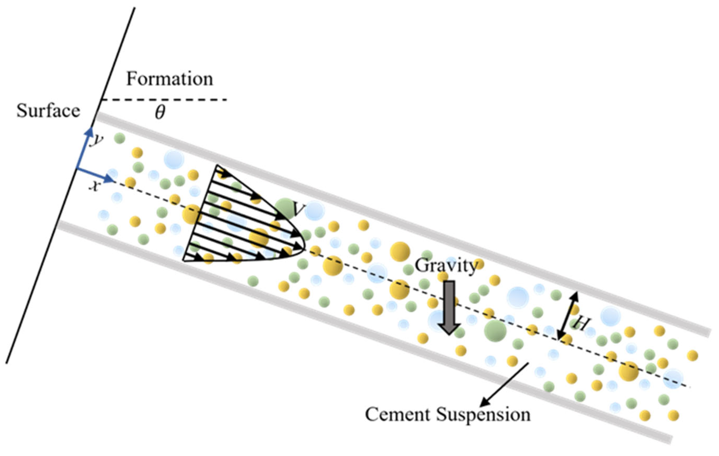
In this study, we consider a representative industrial scenario to evaluate the performance of the proposed model. Drilling operations are typically carried out in either vertical or horizontal orientations. As illustrated in Figure 1, the cement slurry flow is modeled in an inclined channel at an inclination angle with the horizontal axis. The motion of the flow between the two plates of the channel is considered to be fully developed at the steady state.
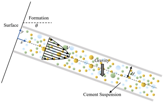
Figure 1.
Flow of cement slurries in the inclined channel.
In the configuration of flow between two inclined plates, the velocity vector is in the e x direction according to the flow motion, and the magnitude of velocity is a function of . The volume fraction is a function of y as well. Equation (9) defines the two variables that need to be solved in the problem.
where represents the unit vector in the motion direction of the cement slurry flow (x-direction). This assumption satisfies the mass conservation Equation (1) and simplifies the momentum and diffusion equations. Equations (1)–(9) are solved, and the dimensionless length and velocity are introduced as:
where H shows the distance between two plates and V is the reference velocity. These equations are finally cast into non-dimensional form:
where is the maximum packing fraction of solid particles, is an experimental parameter (set as 1.82 in this study [45]), and is the power-law exponent. The Heaviside function is defined as for , for . is the coefficient of shear rate, which is related to the magnitude of non-Newtonian behavior such as shear-thickening and shear-thinning; reflects the integrated effect of viscosity and pressure gradient; is the gravitational term; and , , and quantify how the particle volume fraction affects the Brownian diffusive flux in Equation (8). The following dimensionless numbers are defined as
For the boundary conditions of the velocity of cement slurries, a no-slip condition is defined for the velocities at both plates. In dimensionless form, the no-slip boundary conditions at the lower () and upper () plates are shown in Equation (14):
For the boundary condition of the volume fraction of cement slurries, an average quantity is defined, which is expressed as an integral over the cross-sectional area of the flow [46], shown in Equation (15):
The derived equations provide the complete physical framework for constructing the PINN loss function, where the neural network is trained to minimize the residuals of Equations (11) and (12) over the domain and to satisfy boundary constraints (14)–(15). This hybrid approach enables efficient and data-consistent modeling of cement slurry flows under varying operating conditions.
3. Methodology
In this study, the PINN algorithm is applied to analyze the parameters’ influence on the differential equations above. We use a device with an RTX 4060 Ti as the graphics card. The basic environment is built with the Python 3.9, PyTorch 2.1.0, and CUDA 11.8 libraries. The modular interface torch.nn.Module is used to define the network structure. As a starting point, labeled data loss is not considered. We investigate the impact on the results by changing various settings of the neural network, including the structure of the neural networks, training epochs, and learning rate. Then, we conduct a parametric study to evaluate the effect of parameters on the rheological performance (viscosity and volume fraction) of the flow. The parameters include . Finally, we propose the improved methods, including using labeled data and two neural networks trained simultaneously.
3.1. PINN Settings
Figure 2a shows the schematics of the classic PINN algorithms, detailing the PINN employed to solve the non-dimensional Equations (11) and (12) governing cement slurry flow in the tilted channel. The PINN is formulated as a fully connected deep neural network that receives the normalized vertical coordinate as input and predicts the dimensionless velocity and volume fraction as outputs. Figure 2b illustrates the data transformation process between adjacent layers. To calculate the value of for the ith neuron at layer, the weighted sum of the values at layer, together with bias, is multiplied by the nonlinear activation function. By trying various functions such as ReLU, Sigmoid, a hyperbolic tangent () is found to have the optimal performance. Thus, is used as the activation function in all hidden layers. This procedure is expressed in Equation (16):
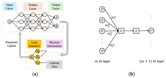
Figure 2.
Schematics of PINN algorithm in solving the non-dimensional ODE system: (a) processes from input data to loss function; (b) data transferring from one layer to the next layer.
Once all the parameters are set, an initial solution from the output layer can be obtained when the data makes the first forward propagation. These solutions are polynomials consisting of weight , bias , and activation function . The objective is to determine the optimal parameters and by minimizing a composite loss function, which combines the residuals of the governing differential equations with the supervised error on any available labeled data. The best solution of and can be achieved by minimizing the loss function. To ensure that the learned solutions respect the underlying physics, the loss function combines three primary components:
- Loss of governing equations (): the residuals of the governing Equations (11) and (12), evaluated across collocation points on the equation solution domain ;
- Loss of boundary conditions (): penalties for violations of the boundary conditions specified in Equations (14) and (15);
- Loss of labeled data (): optional supervised loss using labeled data when available, such as from simulations or experiments, evaluated across known labeled data points for velocity and volume faction
3.2. Performance Metrics
In this study, the mean absolute error of normalized profiles (MAENP) is used to evaluate the trend consistency between two sets of velocity. In contrast to traditional mean absolute error (MAE), which reflects raw magnitude differences. MAENP operates on data that has been individually normalized to the [0, 1] range. This normalization removes scale effects and allows for a pure comparison of shape or trend. This metric is defined as
where and denote the normalized value at a dimensionless position from the PINN prediction and numerical solution, respectively, and is the total number of sampling points across the profile. By focusing solely on the relative trends, MAENP is particularly beneficial in the context of surrogate modeling or neural network predictions, where capturing the global structure of a profile may be more critical than precise pointwise accuracy.
The uniformity of volume fraction in cement slurry plays a critical role in determining the consistency, stability, and mechanical performance of the hardened material. A consistent volume fraction ensures stable viscosity and yield stress throughout the slurry, which is crucial for workability, pumpability, and flow behavior during placement. In this study, the uniformity is measured by a direct metric, defined as the range between the maximum () and minimum () values of volume fraction:
The Uni metric is then used to measure the performance of PINN when compared with other numerical solution by the MAE, as shown in Equation (23):
where is the uniformity of the volume fraction from PINN, is the corresponding uniformity from numerical results, and K is the number of different values for a specific parameter when conducting the parameter study. Uni directly impacts the rheological behavior and microstructural development during setting and hardening, and the MAE metric will help to measure how the PINN captures this important property.
4. Results and Discussion
This section evaluates the performance of the PINN under varying neural network configurations and physical parameter settings. Results are analyzed based on model accuracy, convergence behavior, and agreement with known physical trends.
4.1. Network Architecture Tuning
In this section, the parameters of the ODEs are fixed with
Some settings of neural networks and training methods are chosen as follows: training is performed using the Adam optimizer, which updates network weights based on gradient information. To improve convergence and prevent local minima, a learning rate scheduler is implemented to decay the learning rate over time.
4.1.1. Neural Network Structure
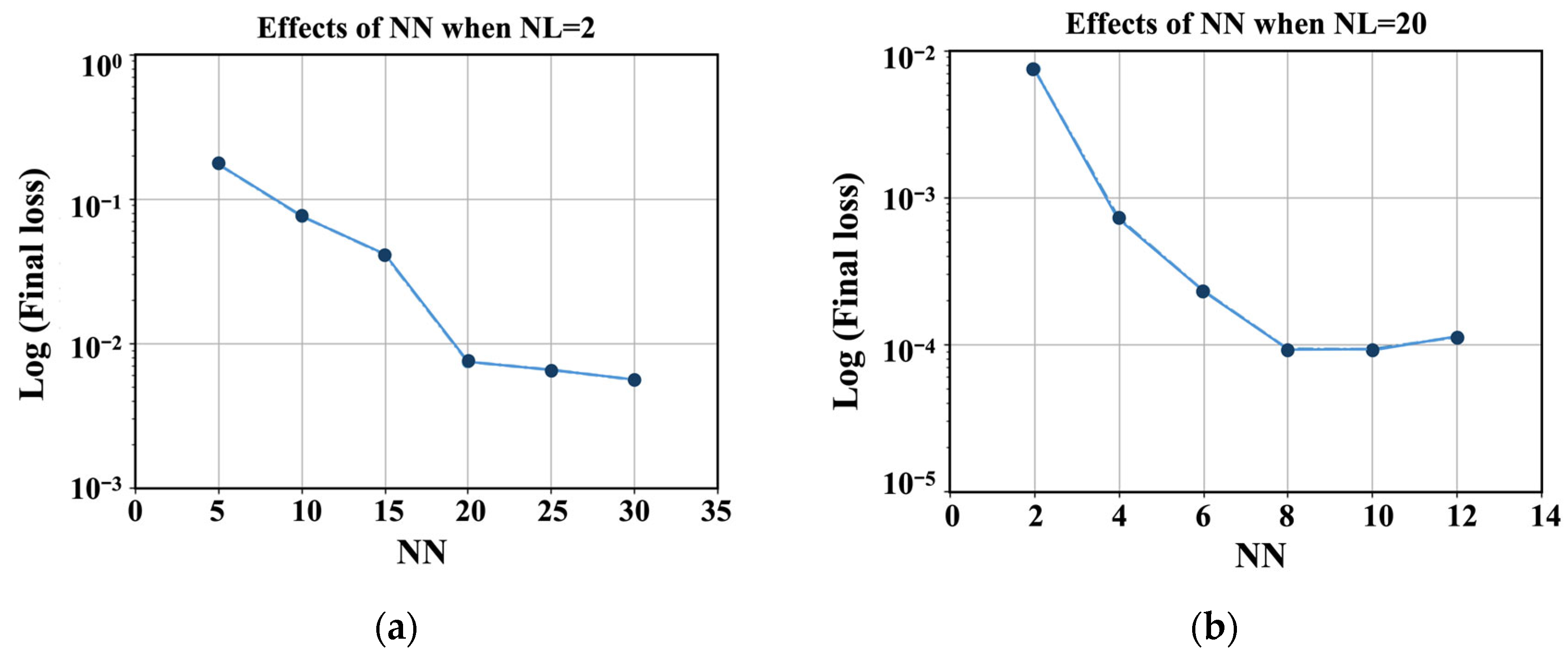
The fitting performance of a PINN mainly depends on the number of hidden layers and how many neurons are there in each layer. We examine the influence of two hyperparameters by parameter tuning. The number of layers (NL) is first set as 2, and the number of neurons (NN) is adjusted. Figure 3a shows how the final loss changes with more neurons in each layer. To express this more clearly, is used to process the final loss. As can be seen in Figure 3, the final loss decreases slowly after NN = 20. For computational efficiency reasons, the number of neurons is set to be 20. It seems the best model still has loss if NL =2 is chosen. To obtain a more accurate solution, the number of hidden layers should also be added. Figure 3b illustrates the trend of the final loss with the change in layer complexity. The total loss can reach when NL = 8 and 10. However, after that, the final loss increases when NL = 12, which may be due to overfitting. Based on these observations, an 8-layer, 20-neuron configuration is adopted for all subsequent experiments.
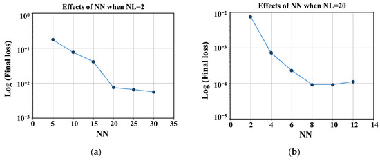
Figure 3.
Effects of NN and NL, with (a) NL = 2 and (b) NN = 20.
4.1.2. Training Epochs and Learning Rate
We also investigate how different learning rates impact training stability and convergence. Minimizing the total loss function requires proper training epochs and learning rate to work together. Small epochs may result in the model training being insufficient or having slow training efficiency. However, while it is too large, the loss function will keep fluctuating near the lowest point. Thus, 5000 training epochs with , , and learning rates are chosen in this portion.
Figure 4 compares the training dynamics of the PINN model under different learning rate settings. The model trained with a learning rate of exhibits rapid initial loss reduction, ultimately failing to converge to a stable solution. In contrast, the learning rate of offers a trade-off between convergence speed and stability, yielding relatively low but fluctuating losses. The most stable and accurate convergence is achieved with a learning rate of which maintains smooth loss decay and achieves the lowest final error. These results suggest that a small learning rate is essential for ensuring stable convergence in PINN training. A dynamic learning rate schedule, starting at and decaying by a factor of 0.9 every 500 steps, yields optimal performance.
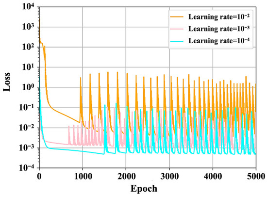
Figure 4.
Training loss over 5000 epochs under learning rate = .
Compared with conventional numerical schemes in the CFD approach, PINN algorithms do not require mesh generation, which simplifies implementation, especially for problems with complex or moving geometries. It has the potential to highly improve the computational cycle and benefits the flexible adjustment. Furthermore, the PINN approach in this study enables continuous and differentiable approximation for the solutions over the entire domain and reduces the requirement for interpolation between discrete nodes in conventional CFD schemes.
4.2. Parametric Studies on Cement Rheology with PINN
We conduct a systematic study to examine how varying key physical parameters affect the flow characteristics. The neural network architecture consists of 8 hidden layers with 20 neurons per layer. A total of 100 training points are uniformly distributed across 1-unit dimensionless distance. The hyperbolic tangent ( is employed as the activation function. The model is optimized using the mean squared error (MSE) loss function, and training begins with a learning rate of by the Adam optimizer.
The indicator for ending training is that the loss function reaches or the 18,000 iteration process are completed. After training the PINN model, all the final loss functions are less than , which indicates relatively good results. All hyperparameters are kept consistent throughout the experiments to ensure comparability.
The parameters we study include the maximum volume fraction , the ratio of empirical coefficients , the inclination angle , the material parameter , and the dimensionless parameters . The following parts show what effects these parameters have with the rest of the parameters fixed.
4.2.1. Effect of
Figure 5 indicates the influence of varying maximum particle volume fraction, , on the trends of velocity and volume fraction. Five values of (0.45, 0.50, 0.55, 0.60, and 0.65) are examined. In all cases, the velocity profile retains its parabolic shape, and the volume fraction consistently concentrates near the mean value at a lower , primarily caused by the first term of the particle flux in Equation (8) of the particle flux. While increases, the dimensionless velocity will increase, and the volume fraction will be more nonuniform. As defined earlier, is the maximum packing fraction of solid particles, where the volume fraction of cement particles aggregates in closest-packing, at which the relative viscosity approaches infinity. At higher , more particles tend to concentrate at the center, resulting in larger velocity and more nonuniformity of cement particles between the two plates. This trend obtained from PINN fits well with the numerical results in reference [3] in a qualitative way. The MAENP value for dimensionless velocity is low at 0.013, suggesting that the PINN reliably captured the overall flow profile trends. The MAE for the uniformity under these five occasions also reaches 0.008, indicating good prediction results. Similar trends in velocity and concentration profiles are reported in reference [47].
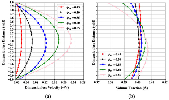
Figure 5.
Effect of on (a) the velocity and (b) the volume fraction, resulting from the PINN solution with , , , , , , , , , , .
4.2.2. Effect of
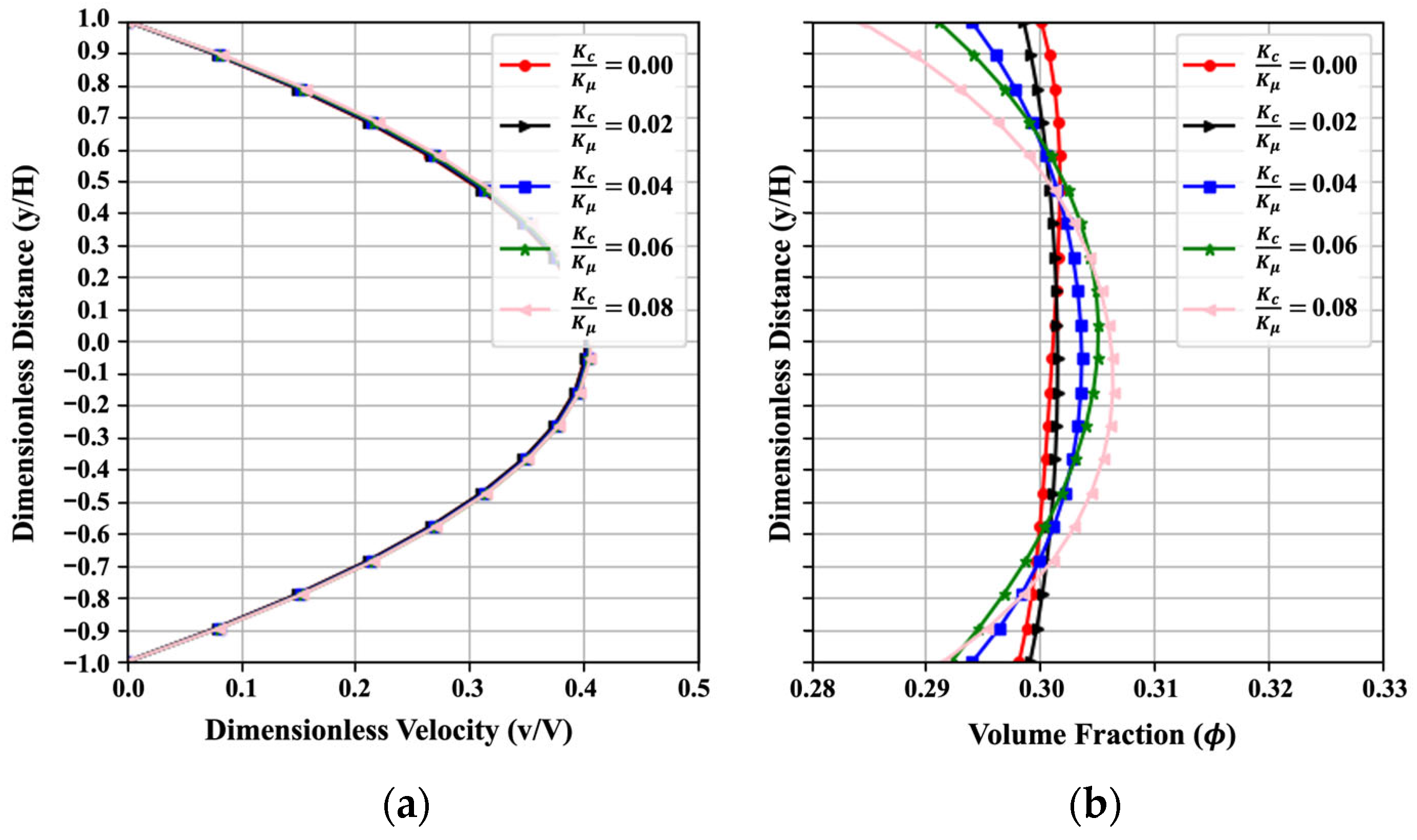
Figure 6 illustrates the influence of the ratio of empirical coefficients on the trends of velocity and volume fraction. As explained in Section 2.2, and are related to the flux terms in cement particle collisions and spatially varying viscosity in Equation (8). A higher value of indicates a higher effect of particle collision compared to the spatial variation of the viscosity. A total of five values within the change from 0.00 to 0.08 are selected for the parametric study. Generally, the velocity shows a parabolic distribution, and the volume fraction tends to concentrate near the value of when is 0. With the increase in , velocity has a very slight increase, and the volume fraction exhibits more nonuniform behavior. An increase in the values of indicates that particles tend to move toward the centerline due to the higher effect of particle collisions. This trend obtained from PINN fits well with the numerical results in reference [3] in a qualitative way. The MAENP value for the dimensionless velocity is as low as 0.003, indicating that the PINN effectively captured the overall flow profile trends. Meanwhile, the MAE for uniformity across the five cases is 0.011, reflecting a satisfactory level of prediction accuracy. And similar trends in velocity and concentration profiles are also reported in reference [47].
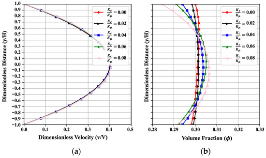
Figure 6.
Effect of on (a) the velocity and (b) the volume fraction, resulting from the PINN solution with , , , , , , , , , , .
4.2.3. Effect of
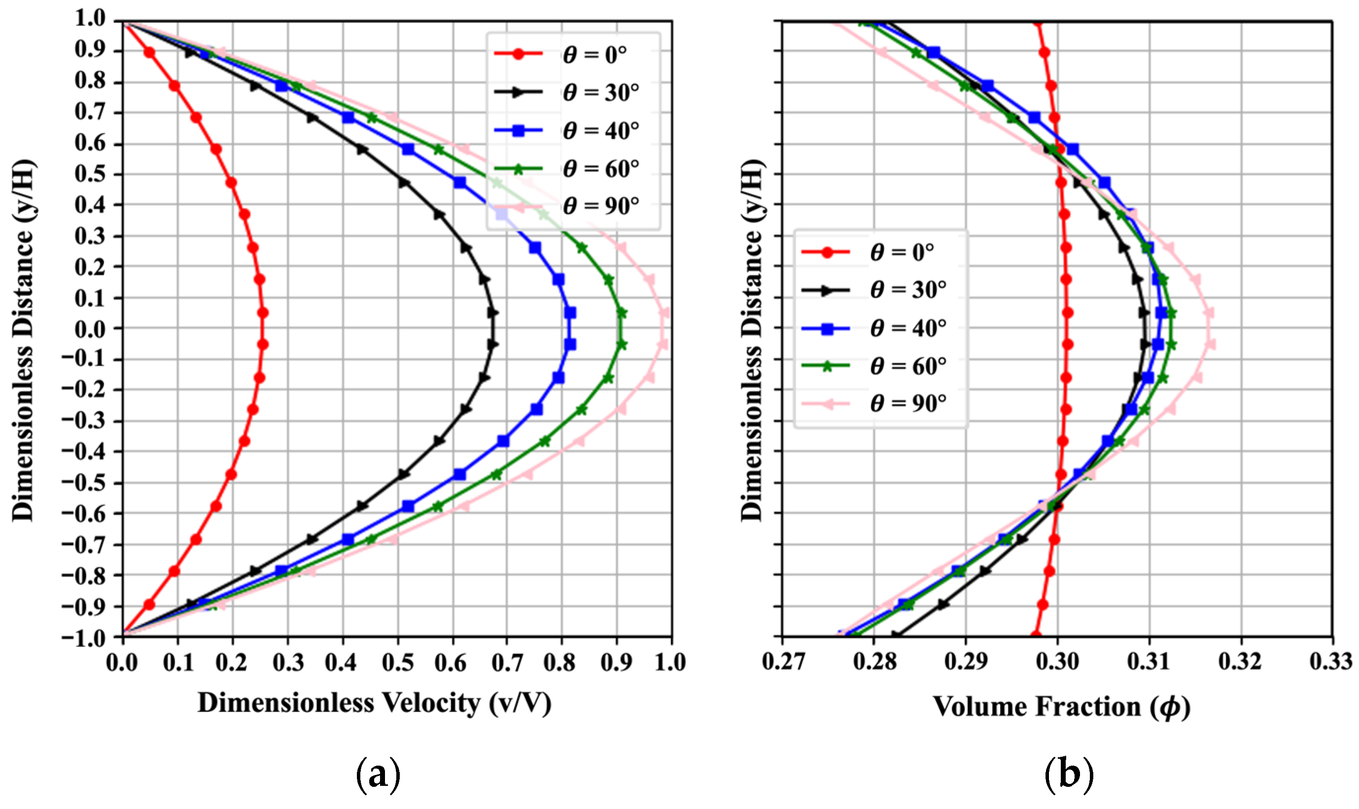
Figure 7 indicates the influence of the inclination angle on the trends of velocity and volume fraction profiles. A total of five values ranging from to are used for the parametric study. For the horizontal setting of two plates, the inclination angle , and when the two plates are in the vertical direction, . The volume fraction tends to concentrate near the value of in the horizontal channel. A larger indicates the increasing gravitational force in the x-direction, which leads to a larger velocity and a more nonuniform volume fraction. Thus, larger plate inclinations result in faster cement slurry flow with increased velocities between the two plates. The cement particles in the flow become more active with higher nonuniformity in the channel. The parametric results can be used to design the channels of offshore oil rigs for better cementing operations with optimal flow behavior of oilwell cement slurries. This trend obtained from PINN fits well with the numerical results in the reference [3] in a qualitative way. A low MAENP of 0.004 for dimensionless velocity demonstrates the PINN’s ability to accurately capture the overall flow pattern. Additionally, the MAE for uniformity under the five scenarios reaches 0.017, showing reliable prediction performance.
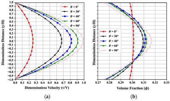
Figure 7.
Effect of on (a) the velocity and (b) the volume fraction, resulting from the PINN solution with .
4.2.4. Effect of
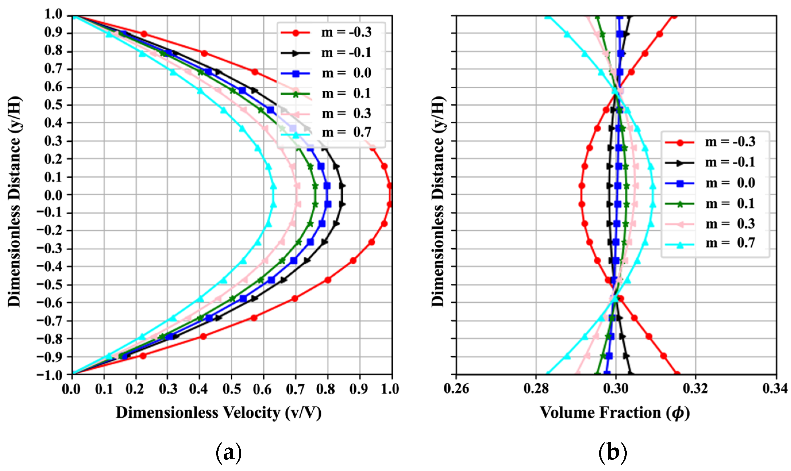
Figure 8 indicates the influence of the material parameter on the trends of velocity and volume fraction with the change from to . To assess the effect of the rheological behavior, both positive and negative values of are investigated. At m = 0, the slurry behaves as a Newtonian fluid, with the viscosity independent of volume fraction; for , it exhibits shear-thinning behavior; and for , it exhibits shear-thickening behavior. Obviously, the velocity curve retains its parabolic shape, and the volume fraction tends to concentrate near the value of at (Newtonian fluid). As m increases from negative to positive, the velocity at the centerline decreases, and the direction of the volume fraction reverses. A larger absolute value of indicates more nonuniform particle concentration. Higher nonlinear behavior (either shear-thinning or shear-thickening) of cement slurries would affect the particle movement and concentration. The results can be a guide for the design of oilwell cement and 3D printing cement by considering the effect of the non-Newtonian fluid behavior of the fresh cement. This trend obtained from PINN fits well with the numerical results in reference [3] in a qualitative way. With an MAENP of just 0.005 for dimensionless velocity, the PINN shows strong capability in reproducing the overall flow behavior. The MAE of 0.032 for uniformity across six cases further confirms the robustness of its predictions. And similar trends in velocity and concentration profiles are also reported in references [47,48].
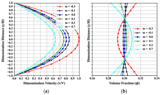
Figure 8.
Effect of on (a) the velocity and (b) the volume fraction, resulting from the PINN solution with .
4.2.5. Effect of
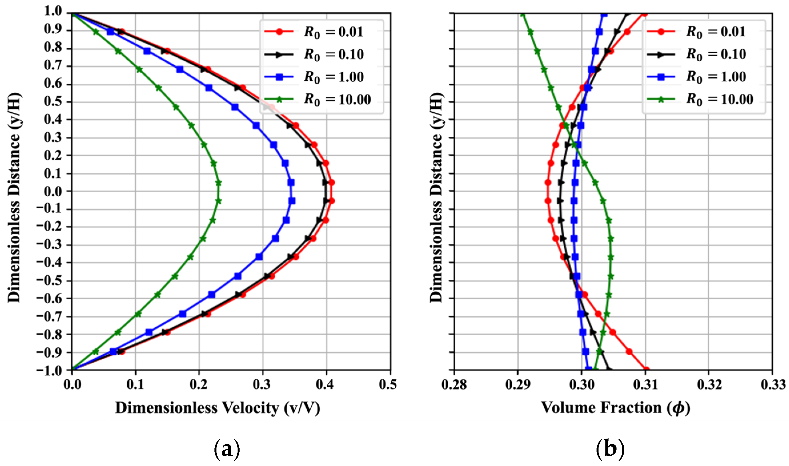
Figure 9 illustrates the influence of the dimensionless parameter on the trends of velocity and volume fraction with the change from to . As defined earlier, corresponds to the shear-rate coefficient that is related to the magnitude of non-Newtonian behavior such as shear-thickening and shear-thinning. Higher indicates weaker non-Newtonian behavior. The velocity generally shows a parabolic distribution. While increases, the dimensionless velocity will decrease, and the distribution of the volume fraction tends to be more nonuniform. The results can be used to determine and optimize the shear rate during oilwell cementing and 3D printing cement and concrete construction practices. This trend obtained from PINN fits well with the numerical results in the reference [3] in a qualitative way. The low MAENP (0.012) for dimensionless velocity suggests that the PINN successfully learned the general flow characteristics. Furthermore, the MAE of 0.012 for uniformity across the four instances indicates that the predictions are both accurate and consistent.
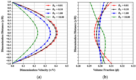
Figure 9.
Effect of on (a) the velocity and (b) the volume fraction, resulting from the PINN solution with .
4.2.6. Effect of
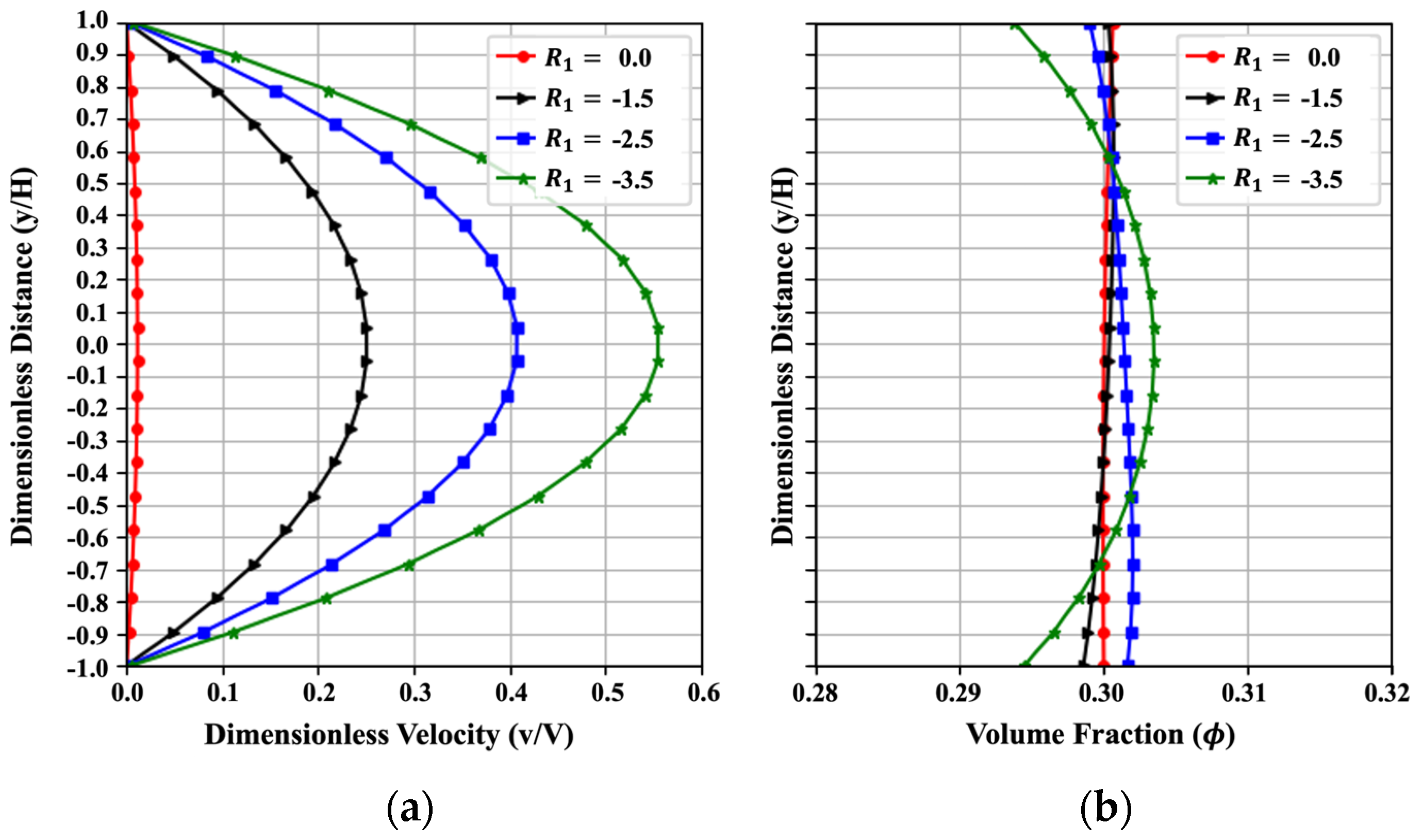
Figure 10 indicates the influence of the dimensionless parameter on the trends of velocity and volume fraction with the change from to . The coefficient quantifies the contributions from viscosity and the pressure gradient. It is related to the effect of the pressure gradient in the x-direction. Generally, the velocity shows a parabolic distribution and the volume fraction tends to concentrate near the value of . While the absolute value of increases, velocity has a significant decrease, and the volume fraction will be more uniform. When , the pressure gradient vanishes, and the volume fraction profile remains uniform. The effect from the pressure gradient term can be used to determine the pumping and vibration rate in cement construction and oilwell cementing. This trend obtained from PINN fits well with the numerical results in the reference [3] in a qualitative way. The dimensionless velocity yields a low MAENP of 0.013, demonstrating that the PINN effectively captured the key flow dynamics. Similarly, an MAE of 0.017 for uniformity in all four scenarios supports the conclusion of reliable and accurate predictions. Similar trends on this pressure gradient effect are shown in References [48,49].
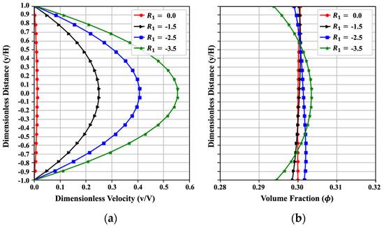
Figure 10.
Effect of on (a) the velocity and (b) the volume fraction, resulting from the PINN solution with .
4.2.7. Effect of
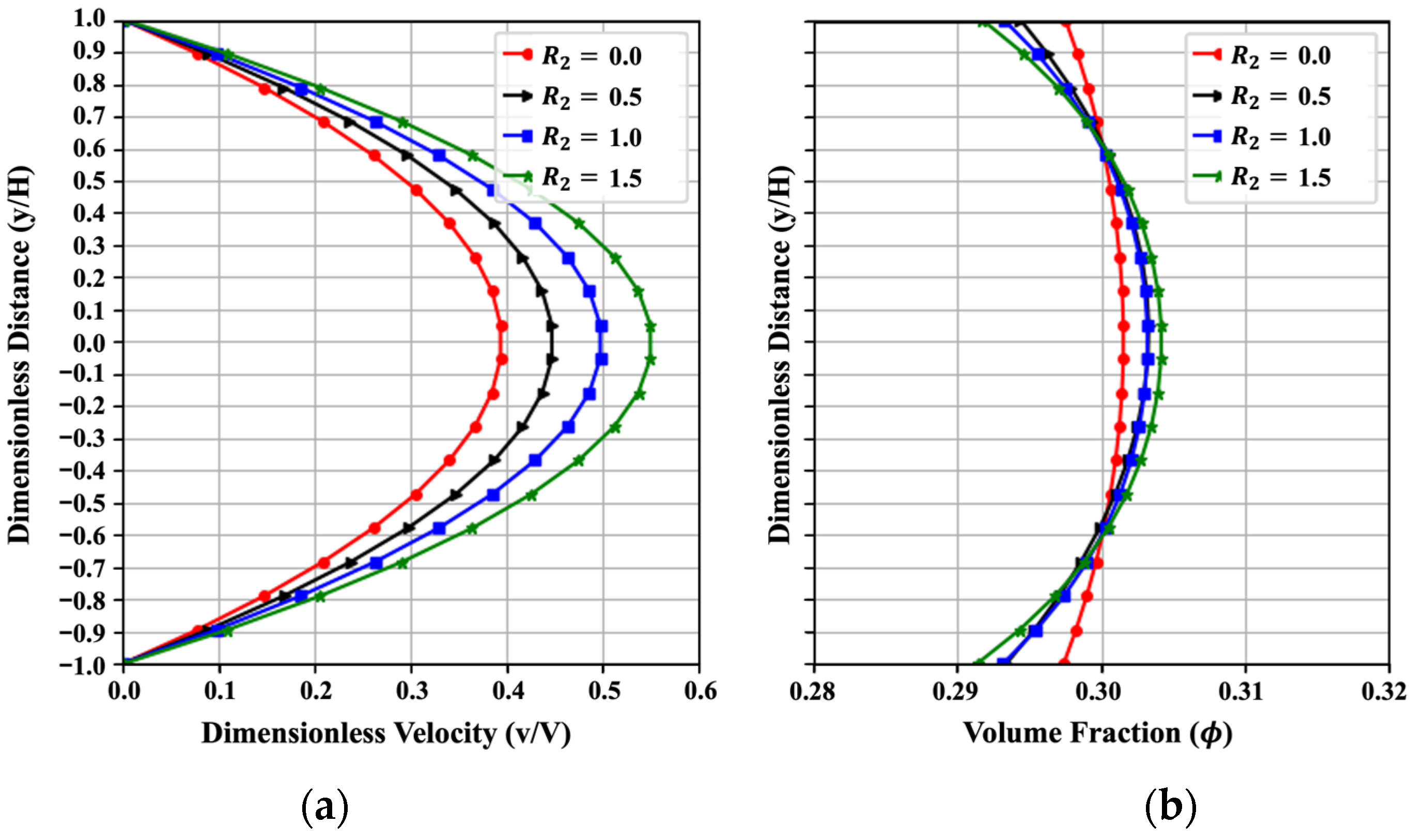
Figure 11 indicates the influence of the dimensionless parameter on the trends of velocity and volume fraction with the change from to . is the gravitational term related to the weight of cement slurries. Generally, the velocity shows a parabolic distribution, and the volume fraction tends to concentrate near the value of at low . With the increase in , the centerline of velocity is higher, and the volume fraction becomes slightly more nonuniform. A higher gravity of cement slurry results in faster flow and higher activation of cement particles, resulting in the phenomenon of velocity and volume fraction profiles. The results would provide insights to determine the pumping or printing frequency to achieve the optimal amount of fresh cement in oilwell cementing and construction. This trend obtained from PINN fits well with the numerical results in references [3] in a qualitative way. The MAENP value for the dimensionless velocity is as low as 0.014, indicating that the PINN effectively captured the overall flow profile trends. Additionally, the MAE for uniformity under the four scenarios reaches 0.009, showing reliable prediction performance. A similar result is also shown in reference [48].
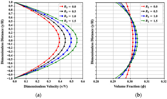
Figure 11.
Effect of on (a) the velocity and (b) the volume fraction, resulting from the PINN solution with .
As shown in Figure 5, Figure 6, Figure 7, Figure 8, Figure 9, Figure 10 and Figure 11, we plot both the dimensionless velocity and volume fraction as predicted by the PINN model and numerical solution. Both of them indicate a regular trend with the change of , , , , and . The trends align with known expectations [3], which proves that these PINNs can capture the trend when conducting a parameter study for cement slurry, through it currently does not have the ability to predict the exact value at different distances . The next section mentions some potential methods that may help to obtain a better result. In general, PINN is a method that combines the advantages of neural networks and physical models, which can effectively solve some complex scientific and engineering problems without labeled data.
4.3. Further Improvements of PINN
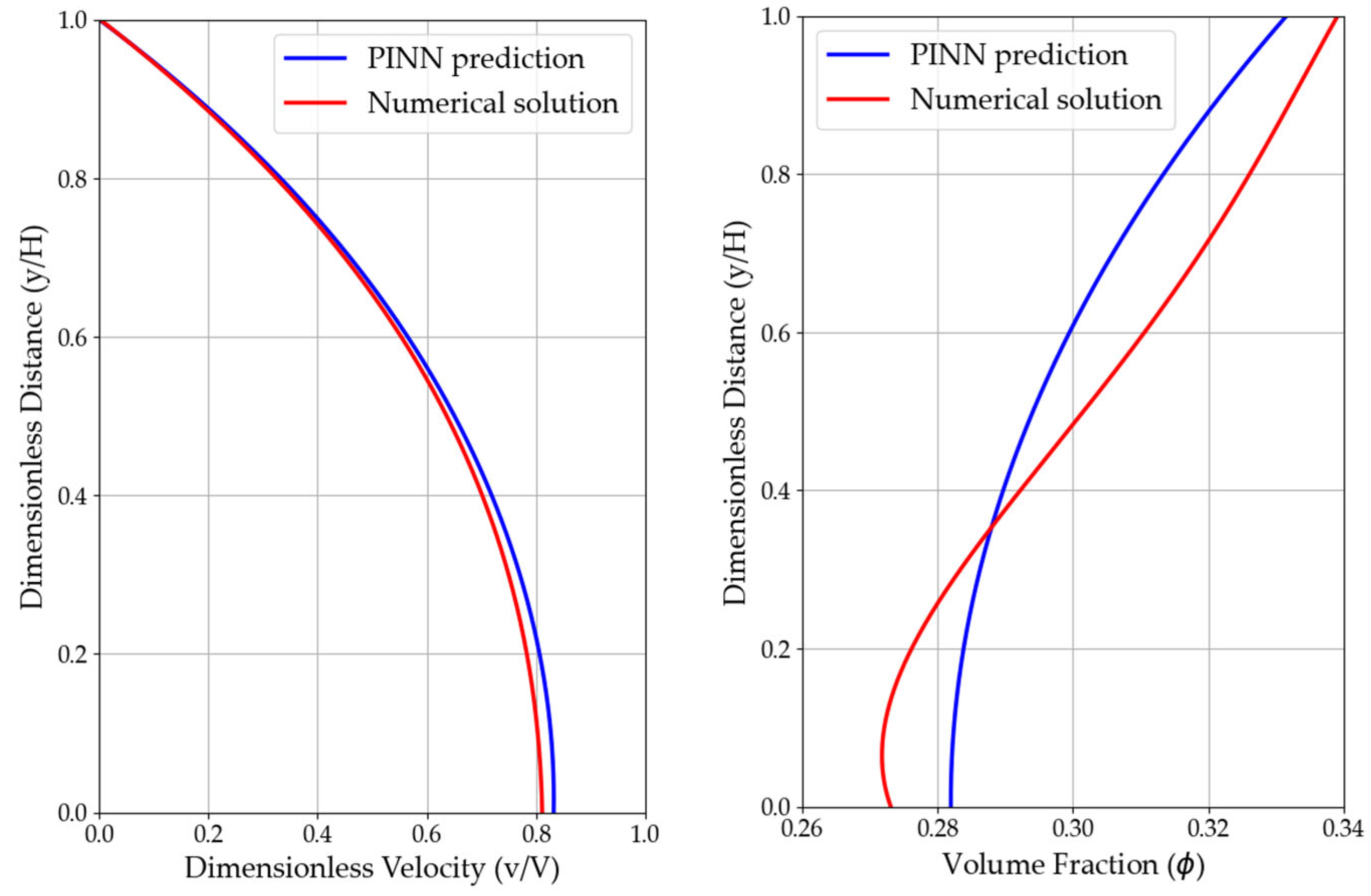
As mentioned before, the precision and reliability of the solution from PINN will be significantly enhanced when some labeled data are considered as a part of the loss function. In this case, we incorporate two known values (centerline velocity and centerline volume fraction) into the loss function, which are obtained from a previous study’s numerical solution [3]. In addition, we experiment with using two separate neural networks () simultaneously instead of using one neural network to simulate two solutions. Figure 12 compares these enhanced models with the original PINN used in previous sections. The MAENP for the velocity prediction reaches 0.003 when compared with the previous research [3], which indicates that the PINN model is capable of accurately reconstructing the dimensionless velocity profile. The most exciting result is that even without the normalization process, the MAE for the velocity prediction can still reach 0.014, indicating the improvement from labeled data and the dual-neural network structure. Meanwhile, the MAE for uniformity is 0.017, reflecting a satisfactory level of prediction accuracy. The dual-network, data-assisted configuration produces smoother curves and better captures profile curvature near the walls. However, it also increases training time and requires additional supervision, which may not always be available.
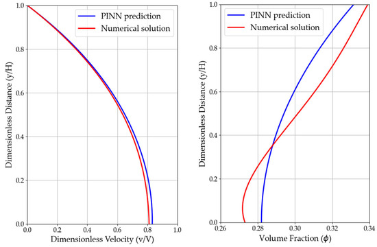
Figure 12.
Improved results of PINN (blue line) compared with a numerical solution (red line).
5. Conclusions and Future Work
This work demonstrates the application of PINN to the steady-state rheological modeling of cement slurry in inclined channel flows. By embedding governing equations, including mass and momentum conservation, non-Newtonian constitutive laws, and particle transport mechanisms into the loss function of a deep neural network, the proposed PINN framework offers a mesh-free, data-efficient approach to solving nonlinear fluid problems relevant to civil engineering. Our study indicates that the PINN successfully captures complex cement slurry behavior governed by material parameters and environmental factors, which is validated through parametric studies against classical numerical solutions. The MAENP for dimensionless velocity remained below 0.014 in all parametric studies, with the best case reaching 0.003. An enhanced model using a dual-network structure and two labeled data points further reduced velocity MAENP to 0.003 and raw MAE to 0.014, demonstrating the benefit of supervised hybrid strategies in improving accuracy. For the prediction of volume fraction uniformity, the PINN achieved MAE values as low as 0.008, confirming its ability to capture critical microstructural variations in cement slurry. In oilwell cementing practice, fundamental understanding and accurate prediction of flow behavior of oilwell cement slurry from the parametric study would help optimize the cement design by enhancing the pumpability, workability, zonal isolation, and long-term oilwell integrity. Key contributions and advantages of the proposed PINN framework include
- Mesh-free modeling: Unlike conventional CFD approaches that rely on meshing and discretization, the PINN approach inherently avoids mesh generation, reducing preprocessing complexity and enabling efficient solutions in geometrically flexible domains.
- Robust trend prediction: Across a variety of parametric conditions, including maximum volume fraction, inclination angle, material coefficients, and dimensionless rheological numbers, the PINN consistently reproduces expected flow and particle concentration profiles with low mean absolute error.
- Data efficiency: The model demonstrates strong generalization without requiring labeled data, yet it allows for precision enhancement by incorporating sparse experimental labels. This balance makes it suitable for data-limited industrial scenarios.
- Modularity and extensibility: The dual-network architecture and hybrid loss function formulation provide a customizable and scalable solution framework for modeling other complex non-Newtonian slurry systems.
Despite the success in steady-state modeling, several opportunities remain for further development. Future work will explore adapting the model for complex annular geometries to better simulate real-world drilling and cementing scenarios. Moreover, combining PINNs with more data-driven surrogate models or transfer learning from CFD datasets may help to accelerate convergence and reduce sensitivity to network hyperparameters. In summary, this work highlights the capability of PINNs to serve as a flexible, accurate, and computationally efficient modeling tool for non-Newtonian cement slurries. The methodology holds promise for advancing intelligent, data-integrated workflows in the design of drilling and construction materials, where physical laws and sparse data must be integrated under practical constraints.
Author Contributions
Conceptualization: C.T.; methodology: H.Y., J.D. and C.T.; PINN modeling: H.Y.; validation: C.T., H.Y. and J.D.; writing—original draft preparation: H.Y., C.T. and J.D.; writing—review and editing: C.T., H.Y. and J.D.; supervision: C.T.; funding acquisition: C.T. All authors have read and agreed to the published version of the manuscript.
Funding
The research was funded by the ACI Foundation (ACIF) Program through its Concrete Research Council (CRC) through Grant No. P0068; the National Science Foundation (NSF) I-Corps through Grant No. TI-2243641; the American Chemical Society Petroleum Research Fund through Grant No. PRF #67005-DNI9; and an Early-Career Research Fellowship from the Gulf Research Program of the National Academies of Sciences, Engineering, and Medicine through Grant No. SCON-10000955. The findings and opinions expressed in this study are those of the authors only and do not necessarily reflect the views of the sponsors.
Data Availability Statement
The original contributions presented in this study are included in the article. Further inquiries can be directed to the corresponding author.
Conflicts of Interest
The authors declare no conflicts of interest.
References
- Tao, C.; Rosenbaum, E.; Kutchko, B.G.; Massoudi, M. A Brief Review of Gas Migration in Oilwell Cement Slurries. Energies 2021, 14, 2369. [Google Scholar] [CrossRef]
- Tao, C.; Kutchko, B.G.; Rosenbaum, E.; Massoudi, M. A Review of Rheological Modeling of Cement Slurry in Oil Well Applications. Energies 2020, 13, 570. [Google Scholar] [CrossRef]
- Tao, C.; Kutchko, B.G.; Rosenbaum, E.; Wu, W.-T.; Massoudi, M. Steady flow of a cement slurry. Energies 2019, 12, 2604. [Google Scholar] [CrossRef]
- Tao, C.; Rosenbaum, E.; Kutchko, B.; Massoudi, M. Pulsating Poiseuille flow of a cement slurry. Int. J. Non-Linear Mech. 2021, 133, 103717. [Google Scholar] [CrossRef]
- Tao, C.; Watts, B.; Ferraro, C.C.; Masters, F.J. A Multivariate Computational Framework to Characterize and Rate Virtual Portland Cements. Comput.-Aided Civ. Infrastruct. Eng. 2019, 34, 266–278. [Google Scholar] [CrossRef]
- Tao, C.; Massoudi, M. On the Flow of a Cement Suspension: The Effects of Nano-Silica and Fly Ash Particles. Materials 2024, 17, 1504. [Google Scholar] [CrossRef]
- Tao, C.; Wang, Q.; Ahmadi, G.; Massoudi, M. Numerical Analysis of Cement Placement into Drilling Fluid in Oilwell Applications. Materials 2025, 18, 3098. [Google Scholar] [CrossRef]
- Dvoynikov, M.V.; Nikitin, V.I.; Kopteva, A.I. Analysis of Methodology for Selecting Rheological Model of Cement Slurry for Determining Technological Parameters of Well Casing. Int. J. Eng. 2024, 37, 2042–2050. [Google Scholar] [CrossRef]
- Guillot, D. 4 Rheology of Well Cement Slurries. In Developments in Petroleum Science; in Well Cementing; Nelson, E.B., Ed.; Elsevier: Amsterdam, The Netherlands, 1990; Volume 28. [Google Scholar] [CrossRef]
- Casson, N. Flow Equation for Pigment-oil Suspensions of the Printing Ink-type. In Rheology of Disperse Systems; Pergamon Press: Oxford, UK, 1959; pp. 84–104. [Google Scholar]
- Parzonka, W.; Vočadlo, J. Méthode de la caractéristique du comportement rhéologique des substances viscoplastiques d’après les mesures au viscosimètre de Couette (modèle nouveau à trois paramètres). Rheol. Acta 1968, 7, 260–265. [Google Scholar] [CrossRef]
- Herschel, W.H.; Bulkley, R. Konsistenzmessungen von Gummi-Benzollösungen. Kolloid-Z. 1926, 39, 291–300. [Google Scholar] [CrossRef]
- Memon, K.R.; Mahesar, A.A.; Baladi, S.A.; Sukar, M.T. Analyzing Cement Rheological Properties Using Different Additive Schemes at High Pressure and High Temperature Conditions. Mehran Univ. Res. J. Eng. Technol. 2020, 39, 466–474. [Google Scholar] [CrossRef]
- Memon, K.R.; Shuker, M.T. Investigating Rheological Properties of High Performance Cement System for Oil Wells. Res. J. Appl. Sci. Eng. Technol. 2013, 6, 3865–3870. [Google Scholar] [CrossRef]
- Tariq, Z.; Murtaza, M.; Mahmoud, M. Development of New Rheological Models for Class G Cement with Nanoclay as an Additive Using Machine Learning Techniques. ACS Omega 2020, 5, 17646–17657. [Google Scholar] [CrossRef] [PubMed]
- Dissanayake, M.W.M.G.; Phan-Thien, N. Neural-network-based approximations for solving partial differential equations. Commun. Numer. Methods Eng. 1994, 10, 195–201. [Google Scholar] [CrossRef]
- Lagaris, I.E.; Likas, A.C.; Papageorgiou, D.G. Neural-network methods for boundary value problems with irregular boundaries. IEEE Trans. Neural Netw. 2000, 11, 1041–1049. [Google Scholar] [CrossRef]
- Aarts, L.; van der Veer, P. Solving nonlinear differential equations by a neural network method. In Proceedings of the Computational Science International Conference, San Fransisco, CA, USA, 28–30 May 2001; pp. 181–189. [Google Scholar]
- Raissi, M.; Perdikaris, P.; Karniadakis, G.E. Physics-informed neural networks: A deep learning framework for solving forward and inverse problems involving nonlinear partial differential equations. J. Comput. Phys. 2019, 378, 686–707. [Google Scholar] [CrossRef]
- Eivazi, H.; Wang, Y.; Vinuesa, R. Physics-informed deep-learning applications to experimental fluid mechanics. Meas. Sci. Technol. 2024, 35, 075303. [Google Scholar] [CrossRef]
- Lee, J.; Shin, S.; Kim, T.; Park, B.; Choi, H.; Lee, A.; Choi, M.; Lee, S. Physics informed neural networks for fluid flow analysis with repetitive parameter initialization. Sci. Rep. 2025, 15, 16740. [Google Scholar] [CrossRef]
- Bandai, T.; Ghezzehei, T.A. Physics-Informed Neural Networks with Monotonicity Constraints for Richardson-Richards Equation: Estimation of Constitutive Relationships and Soil Water Flux Density From Volumetric Water Content Measurements. Water Resour. Res. 2021, 57, e2020WR027642. [Google Scholar] [CrossRef]
- Han, J.; Nica, M.; Stinchcombe, A.R. A derivative-free method for solving elliptic partial differential equations with deep neural networks. J. Comput. Phys. 2020, 419, 109672. [Google Scholar] [CrossRef]
- Almajid, M.M.; Abu-Al-Saud, M.O. Prediction of porous media fluid flow using physics informed neural networks. J. Pet. Sci. Eng. 2022, 208, 109205. [Google Scholar] [CrossRef]
- Cuomo, S.; Di Cola, V.S.; Giampaolo, F.; Rozza, G.; Raissi, M.; Piccialli, F. Scientific Machine Learning Through Physics–Informed Neural Networks: Where we are and What’s Next. J. Sci. Comput. 2022, 92, 88. [Google Scholar] [CrossRef]
- Meng, Z.; Qian, Q.; Xu, M.; Yu, B.; Yıldız, A.R.; Mirjalili, S. PINN-FORM: A new physics-informed neural network for reliability analysis with partial differential equation. Comput. Methods Appl. Mech. Eng. 2023, 414, 116172. [Google Scholar] [CrossRef]
- Krishnapriyan, A.S.; Gholami, A.; Zhe, S.; Kirby, R.M.; Mahoney, M.W. Characterizing possible failure modes in physics-informed neural networks. arXiv 2021, arXiv:2109.01050. [Google Scholar] [CrossRef]
- Wang, S.; Sankaran, S.; Perdikaris, P. Respecting causality for training physics-informed neural networks. Comput. Methods Appl. Mech. Eng. 2024, 421, 116813. [Google Scholar] [CrossRef]
- Lawal, Z.K.; Yassin, H.; Lai, D.T.C.; Che Idris, A. Physics-Informed Neural Network (PINN) Evolution and Beyond: A Systematic Literature Review and Bibliometric Analysis. Big Data Cogn. Comput. 2022, 6, 140. [Google Scholar] [CrossRef]
- Reyes, B.; Howard, A.A.; Perdikaris, P.; Tartakovsky, A.M. Learning unknown physics of non-Newtonian fluids. Phys. Rev. Fluids 2021, 6, 073301. [Google Scholar] [CrossRef]
- Liu, K.; Luo, K.; Cheng, Y.; Liu, A.; Li, H.; Fan, J.; Balachandar, S. Parameterized physics-informed neural networks (P-PINNs) solution of uniform flow over an arbitrarily spinning spherical particle. Int. J. Multiph. Flow 2024, 180, 104937. [Google Scholar] [CrossRef]
- Lu, D.; Christov, I.C. Physics-informed neural networks for understanding shear migration of particles in viscous flow. Int. J. Multiph. Flow 2023, 165, 104476. [Google Scholar] [CrossRef]
- Zhang, T.; Wang, D.; Lu, Y. RheologyNet: A physics-informed neural network solution to evaluate the thixotropic properties of cementitious materials. Cem. Concr. Res. 2023, 168, 107157. [Google Scholar] [CrossRef]
- Banfill, P.F.G.; Kitching, D.R. 14 Use of a controlled stress rheometer to study the yield stress of oilwell cement. In Rheology of Fresh Cement and Concrete: Proceedings of an International Conference, Liverpool, 1990; CRC Press: London, UK, 1990; p. 125. [Google Scholar]
- Struble, L.; Sun, G.-K. Viscosity of Portland cement paste as a function of concentration. Adv. Cem. Based Mater. 1995, 2, 62–69. [Google Scholar] [CrossRef]
- Foroushan, H.K.; Ozbayoglu, E.M.; Miska, S.Z.; Yu, M.; Gomes, P.J. On the instability of the cement/fluid interface and fluid mixing. SPE Drill. Complet. 2018, 33, 63–76. [Google Scholar] [CrossRef]
- Skadsem, H.J.; Kragset, S.; Lund, B.; Ytrehus, J.D.; Taghipour, A. Annular displacement in a highly inclined irregular wellbore: Experimental and three-dimensional numerical simulations. J. Pet. Sci. Eng. 2019, 172, 998–1013. [Google Scholar] [CrossRef]
- Liu, L.; Fang, Z.; Qi, C.; Zhang, B.; Guo, L.; Song, K.-I. Numerical study on the pipe flow characteristics of the cemented paste backfill slurry considering hydration effects. Powder Technol. 2019, 343, 454–464. [Google Scholar] [CrossRef]
- Slattery, J.C. Advanced Transport Phenomena; Cambridge University Press: Cambridge, UK, 1999. [Google Scholar]
- Probstein, R.F. Physicochemical Hydrodynamics: An Introduction; John Wiley & Sons: Hoboken, NJ, USA, 2005. [Google Scholar]
- Rivlin, R.S. Further Remarks on the Stress-Deformation Relations for Isotropic Materials. In Collected Papers of R.S. Rivlin; Barenblatt, G.I., Joseph, D.D., Eds.; Springer: New York, NY, USA, 1997; pp. 1014–1035. [Google Scholar] [CrossRef]
- Truesdell, C.; Noll, W. The Non-Linear Field Theories of Mechanics. In The Non-Linear Field Theories of Mechanics; Antman, S.S., Ed.; Springer: Berlin/Heidelberg, Germany, 2004; pp. 1–579. [Google Scholar] [CrossRef]
- Massoudi, M.; Vaidya, A. On some generalizations of the second grade fluid model. Nonlinear Anal. Real World Appl. 2008, 9, 1169–1183. [Google Scholar] [CrossRef]
- Li, Y.; Wu, W.-T.; Liu, X.; Massoudi, M. The effects of particle concentration and various fluxes on the flow of a fluid-solid suspension. Appl. Math. Comput. 2019, 358, 151–160. [Google Scholar] [CrossRef]
- Phillips, R.J.; Armstrong, R.C.; Brown, R.A.; Graham, A.L.; Abbott, J.R. A constitutive equation for concentrated suspensions that accounts for shear-induced particle migration. Phys. Fluids Fluid Dyn. 1992, 4, 30–40. [Google Scholar] [CrossRef]
- Massoudi, M. Boundary conditions in mixture theory and in CFD applications of higher order models. Comput. Math. Appl. 2007, 53, 156–167. [Google Scholar] [CrossRef]
- Wu, W.-T.; Massoudi, M. Heat transfer and dissipation effects in the flow of a drilling fluid. Fluids 2016, 1, 4. [Google Scholar] [CrossRef]
- Miao, L.; Massoudi, M. Heat transfer analysis and flow of a slag-type fluid: Effects of variable thermal conductivity and viscosity. Int. J. Non-Linear Mech. 2015, 76, 8–19. [Google Scholar] [CrossRef]
- Gudhe, R.; Yalamanchili, R.C.; Massoudi, M. The flow of granular materials in a pipe: Numerical solutions. ASME Appl. Mech. Div.-Publ.-AMD 1993, 160, 41. [Google Scholar]


Disclaimer/Publisher’s Note: The statements, opinions and data contained in all publications are solely those of the individual author(s) and contributor(s) and not of MDPI and/or the editor(s). MDPI and/or the editor(s) disclaim responsibility for any injury to people or property resulting from any ideas, methods, instructions or products referred to in the content. |
© 2025 by the authors. Licensee MDPI, Basel, Switzerland. This article is an open access article distributed under the terms and conditions of the Creative Commons Attribution (CC BY) license (https://creativecommons.org/licenses/by/4.0/).