Article

DEM/CFD Simulations of a Pseudo-2D Fluidized Bed: Comparison with Experiments

1
IFP Energie Nouvelles, Rond-Point de l’échangeur de Solaize, BP 3, 69360 Solaize, France
2
CORIA, CNRS, INSA & Université de Rouen, 76801 Saint-Etienne-du-Rouvray, France
*
Author to whom correspondence should be addressed.
Fluids 2019, 4(1), 51; https://doi.org/10.3390/fluids4010051
Submission received: 12 February 2019 / Accepted: 4 March 2019 / Published: 15 March 2019
(This article belongs to the Special Issue Drop, Bubble and Particle Dynamics in Complex Fluids )

Abstract

:
The present work investigates the performance of a mesoscopic Lagrangian approach for the prediction of gas-particle flows under the influence of different physical and numerical parameters. To this end, Geldart D particles with 1 mm diameter and density of 2500 kg/m 3 are simulated in a pseudo-2D fluidized bed using a Discrete Element Method (DEM)/Large-Eddy Simulation (LES) solver called YALES2. Time-averaged quantities are computed and compared with experimental results reported in the literature. A mesh sensitivity analysis showed that better predictions regarding the particulate phase are achieved when the mesh is finer. This is due to a better description of the local and instantaneous gas-particle interactions, leading to an accurate prediction of the particle dynamics. Slip and no slip wall conditions regarding the gas phase were tested and their effect was found negligible for the simulated regimes. Additional simulations showed that increasing either the particle-particle or the particle-wall friction coefficients tends to reduce bed expansion and to initiate bubble formation. A set of friction coefficients was retained for which the predictions were in good agreement with the experiments. Simulations for other Reynolds number and bed weight conditions are then carried out and satisfactory results were obtained.

1. Introduction

Based on their effectiveness regarding gas-solid heat and mass transfers, fluidized beds are among the best options for developing economically and environmentally viable techniques for fossil-fuel-based energy generation. Such systems involve complex physical mechanisms such as momentum, heat and mass exchanges between the gas and the particulate phases. In addition, fluidized beds exhibit an unsteady and inhomogeneous behavior leading to wide characteristic length and time scales. Particle-particle and gas-particle interactions at the micro-scale (1 to 5 d p , where d p is the characteristic length of a particle) result in meso-scale structures, such as bubbles (10 to 100 d p ), which can affect the macro-scale gas-particle flow [1]. Further, different local behaviors can be observed depending on the local particle-particle, gas-particle and particle-wall interactions, and may profoundly modify the bed hydrodynamics. Therefore, various numerical approaches have been developed over the past decades to simulate those flows at microscopic, mesoscopic and macroscopic scales with the aim of elucidating the mechanisms underlying the origin and the evolution of the heterogeneous gas-particle flow pattern. The accurate prediction of the underlying physics makes possible to improve existing processes and to design more efficient new facilities. In this context, the development of reliable numerical approaches is an essential prerequisite.
Discrete Element Method (DEM) is among the most appropriate meso-scale approaches to simulate small scale fluidized beds, with O ( 10 6 ) particles [2]. In this technique the particle motion is given by the Newtonian equations. Particles interact with each others through collisions, that can be described using models from molecular dynamics [3], the so-called sphere models [4,5,6]. In this work the particles are considered as soft spheres that can overlap slightly and exert both normal and tangential forces on each other [4]. This model, known as the soft-sphere model, requires a contact force model in order to account for the inter-particle collision dynamics. The gas flow is solved on an Eulerian grid using a continuum approach based on a volume averaging of the Navier-Stokes equations [7]. Interphase momentum transfer terms are included in the modeling to account for the fluid-particle interactions [8]. In this work, the ability of a DEM/LES approach to reproduce the gas-particle flow behavior in a 2D-fluidized bed is assessed. A specific attention will be paid to the influence of numerical (grid cell size) and physical parameters (friction coefficient).
In Section 2, the modeling strategy is given. Detailed models, based on averaged Navier-Stokes equations for the gas phase, DEM technique for the particles and coupling procedure between the phases are provided in Section 2.1, Section 2.2 and Section 2.3, respectively. Detailed information about the numerical schemes can be found in Section 2.4. Finally, an overview of the simulation cases is presented in Section 3 and results discussed in Section 4.

2. Modeling Strategy

All the numerical simulations presented in this work are performed using the finite-volume code YALES2 [9], a Large-Eddy Simulation (LES) and Direct Numerical Simulation (DNS) solver based on unstructured meshes. This code solves the low-Mach number Navier-Stokes equations for turbulent reactive flows using a time-staggered projection method for constant [10] or variable density flows [11]. YALES2 is specifically tailored for solving these low-Mach number equations on massively parallel machines with billion-cell meshes thanks to a highly optimized linear solvers [12].
Recently, a meso-scale four-way coupling approach for the modeling of solid particles has been implemented in the YALES2 solver. This approach combines DEM approach to represent the solid phase with LES equations solved on an Eulerian unstructured grid for the fluid phase. The CFD/DEM solver has been thoroughly optimized for massively parallel computing. It features a dynamic collision detection grid for unstructured meshes and packing/unpacking of the halo data for non-blocking Message Passing Interface (MPI) exchanges.

2.1. Gas Phase Modeling

The governing equations for the averaged fluids flow are obtained from the filtering of the unsteady, low-Mach number Navier-Stokes equations, taking the local fluid and solid fractions into account. If G is a filtering kernel (see for instance [7]), the local fluid fraction ε is defined as:
ε ( x , t ) = V f G ( | x y | ) d y ,
where V f is the volume occupied by the fluid. Defining Φ ( x , t ) as a function of position and time, the volume filtered field < Φ > ( x , t ) refers to the regular spatial average and is computed by taking the convolution product with the filtering kernel G, giving:
ε < Φ > ( x , t ) = V f Φ ( y , t ) G ( | x y | ) d y .
Further details concerning the volume filtering operations can be found in [8]. The governing equations finally read:
ε t + · ε < u > = 0 ,
ρ t ε < u > + ρ · ε < u > < u > = < P > + · ε < τ > + ε ρ g + 1 Δ V < F > p f ,
u , ρ , P, and τ are the gas velocity, density, dynamic pressure respectively and viscous stress tensor. The closure used to calculate the turbulent viscosity μ t is the localized dynamic Smagorinsky model [13] proposed by [14,15]. The term F ¯ p f is the momentum source term due to particle displacement. Δ V is the local control volume. Details concerning the computation of this term can be found in Section 2.3. For the sake of clarity, the notation < > will be dropped for the averaged quantities in the following.
The use of the LES model for CFD/DEM simulations in case of dense granular flows is questionable. Indeed, there are very few publications dealing with the effect of inertial particles on a turbulent flow in a confined domain. It is thus very difficult to conclude whether the actual flow is turbulent or not. Nevertheless, previous publications (see, for instance, [8]) used this kind of model in fluidized bed simulations. In our case the bulk Reynolds number based on the bed width is relatively high ( 5600 R e 8000 ) so that, a single gas-phase flow in the same condition, is likely to be turbulent or at least in a transition regime. We performed a series of additional computations in order to assess the effect of the turbulent viscosity on the bed hydrodynamics. Results showed that, both qualitatively and quantitatively, such a model did not change significantly the hydrodynamics of the fluidized bed (see Appendix A). This tends to confirm that in the present configuration, the global behaviour of the flow is driven by the largest scales and by particle-particle contact.

2.2. Discrete Particle Modeling

The forces acting on a particle in motion can be divided into two categories, volume and surface forces. The unique volume force in the present situation is the weight whereas, the surface forces consist of hydrodynamic and contact forces. While the hydrodynamic forces arise from fluid-particle interactions, such as drag and lift forces, the contact forces are due to particle-particle and particle-wall interactions. Such forces can be further classified in collision and adhesive forces. In the present work, due to the high solid/gas density ratio, as reported in Table 1, buoyancy, lift and added mass forces are neglected. To date, theoretical expressions for the history force in dense regimes are still missing. Therefore, such a force is not taken into account in our modeling. Concerning the contact forces, only collision forces are accounted for. Adhesive effects that may originate from electrostatic or Van Der Vaals forces can safely be here neglected since, as it can be seen in Table 1, the simulated particles are relatively large (Geldart D particles).
Discrete particle models, in which each particle is tracked is tracked in a Lagrangian fashion, have clearly shown their ability to simulate the behavior of granular flows, and originate from molecular dynamics methods initiated in the 1950s [3]. A soft-sphere model [16] is employed to compute contact between each particle. They are allowed to overlap other particles or walls in a controlled manner. A resulting contact force accounting for particle-particle and particle-wall repulsion is thus added in the momentum balance of each particle. Particle movement is then given by Newton’s second law for translation assuming high solid/gas density ratio:
m p d u p d t = F D + F G + F P + F C with d x p dt = u p ,
where m p , u p , and x p are the particle mass, velocity, position respectively. F D is the drag force, F G is the gravity force, F P is the pressure gradient force and F C is the collision force. The relation between F D , F C in Equation (5) and F p f in Equation (4) is detailed in Section 2.3. Preliminary simulations including particle rotation provided similar results as those without rotation. As a consequence, for computational reason, the particle rotation is not accounted for in this paper.

2.2.1. Modeling of Collisions

The total collision force F C acting on particle a is computed as the sum of all forces f b a c o l exerted by the N p particles and N w walls in contact. As particles and walls are treated similarly during collisions, the b index refers to both:
F C = b = 1 N p + N w f b a c o l ,
f b a c o l = f n , b a c o l + f t , b a c o l .
Depending on the desired compromise between accuracy and numerical cost, a lot of soft sphere models can be found in the literature. Here, a linear-spring/dashpot [16] is used along with a simple Coulomb sliding model accounting for the normal f n , b a c o l and tangential f t , b a c o l components of the contact force, respectively, as in the work of Capecelatro [8]. For one particle (or wall) b acting on a particle a:
f n , b a c o l = k n δ a b n a b 2 γ n M a b u a b , n if δ a b > 0 , 0 else ,
f t , b a c o l = μ t a n | | f n , b a c o l | | t a b .
The term δ a b is defined as the overlap between the a and b entities expressed using each particle radius r p and center coordinates x p such as:
δ a b = r a + r b ( x b x a ) . n a b .
The system effective mass M a b is expressed using each particle mass m p such as:
M a b = 1 1 / m a + 1 / m b .
In case of a particle-wall collision, the wall is considered as a particle with infinite mass and null radius. This model requires three user-defined parameters; k n , γ n , and μ t a n respectively accounting for the spring stiffness, normal damping, and friction coefficient of the a b binary system. n a b and t a b respectively account for the unit normal vector from particle a towards entity b and the unit tangential vector. n a b is calculated as follows:
n a b = x b x a | | x b x a | | .
with u a b being the relative velocity of the colliding system, its normal and tangential components are then given by:
u a b , n = ( ( u a u b ) . n a b ) n a b ,
u a b , t = u a b u a b , n .
Finally, t a b is given by:
t a b = u a b , t | | u a b , t | | .
Using Newton’s third law and a projection on n a b yields the following ordinary differential equation for the overlap evolution of an a b binary system undergoing collision without taking any other force into account:
d 2 δ a b d t 2 + 2 γ n d δ a b d t + ω 0 2 δ a b = 0 ,
where ω 0 stands for the system’s natural frequency and is defined as:
ω 0 2 = k n M a b .
The damping parameter γ n accounting for the energy dissipation occurring during contact is calculated by the mean of a normal restitution coefficient e n verifying 0 < e n 1 such as:
γ n = ω 0 ln e n π 2 + ( ln e n ) 2 .
A contact time T C can also be analytically extracted from Equation (16) corresponding to the time during which the particle a and the entity b are overlapping:
T C = π ω 0 2 γ n 2 .

2.2.2. Closure for Drag

The drag force F D acting on a particle p is written:
F D = m p τ p ( u @ p u p ) ,
where u @ p is the local gas velocity interpolated at the center of the particle p and τ p is the drag relaxation time expressed as follows:
τ p = 4 ρ p d p 2 3 μ C D R e p with R e p = ε @ p ρ | | u @ p u p | | d p μ ,
where ρ p is the particle density, d p its diameter, μ the dynamic viscosity, ε @ p is the local fluid fraction interpolated at the center of the particle, and C D is the drag coefficient. In order to compute C D , the classical closures proposed by Ergun ( C D , E R ) [17] for high ε @ p values and Wen & Yu ( C D , W Y ) [18] for low ε @ p values are used along with the smoothing function ϕ g s introduced by Huilin & Gidaspow [19] to avoid discontinuities when switching models:
ϕ g s = 1 π arctan ( 150 × 1.75 ( 0.2 ( 1 ε @ p ) ) ) + 0.5 ,
in such a way that:
C D = ϕ g s C D , W Y + ( 1 ϕ g s ) C D , E R ,
with
C D , W Y = 24 R e p 1 + 0 . 15 R e p 0 . 687 ε @ p 2.7 for R e p < 10 3 , 0 . 44 ε @ p 2.7 for R e p 10 3 ,
and
C D , E R = 200 1 ε @ p R e p + 7 3 ε @ p 1 .

2.2.3. Other Forces

The gravity force F G acting on a particle p is written:
F G = m p g .
The pressure gradient force F P in Equation (5) reads as:
F P = V p P @ p ,
where V p is the particle’s volume and P @ p is the local pressure gradient interpolated at the center of the particle.

2.3. Phase Coupling

The coupling between the particle and fluid phases is a key point for the modeling of particle-laden flows, especially when the particle size approaches the Eulerian cell size. Many Eulerian fields have to be interpolated at the center of the particles for the numerous closures, as shown in Section 2.2. In the YALES2 solver, particles are located in a unique mesh cell (C) using the position of their center. For any Eulerian scalar or vector field Φ ( x , t ) , its value taken at the particle p center Φ @ p ( t ) obeys:
Φ @ p ( t ) = i C ω p , i Φ ( x , t ) with i C ω p , i = 1 .
Here i is a node index so that ‘ i C ’ means ‘all nodes composing the mesh cell C in which the particle p is located’. ω p , i is the interpolation weight of the particle p on cell node i and is calculated using a trilinear interpolation on tetrahedra and on hexahedra. The same interpolation weights are used for data transfer from grid to particles (interpolation step) and from particle onto the grid (projection step).
The conservative projection operator needed to compute F p f (see Equation (4)) is thus written on each node i as:
F p f , i = p S C i ω p , i ( F D + F P ) ,
and the fluid fraction at node i is written:
ε i = 1 Δ V i p S C i ω p , i V P .
Here Δ V i denotes the control volume of node i and ‘ p S C i ’ means ‘all particles belonging to any surrounding cell (SC) of node i’. Referring to Figure 1, it means that any particle belonging to one of the cells will be accounted for when computing ε (as well as F p f ) at node 3.
This method consisting in distributing particle quantities only in the cell where its center resides, referred to as Particle Centroid Method (PCM), can lead to large calculation errors in particular regarding the fluid fraction, as pointed out in [20]. This is partly due to the fact that many CFD/DEM codes feature a staggered grid where the fluid fraction is defined at cell centers, causing dramatic discontinuities in time and space derivatives when a particle enters or leaves a cell. On the contrary, in the YALES2 code the fluid fraction, as all the Eulerian fields, is computed at the grid nodes. As depicted in Figure 1, it is then straightforward that the particle crossing from the green cell to the red one won’t cause any discontinuity on the computation of neither ω p , 1 nor ω p , 3 involved in their interface. Moreover ω p , 2 won’t be much affected neither during the crossing because as the particle approaches the cell’s interface, ω p , 2 tends towards 0. This is still true in 3D cases and on Cartesian meshes.
Nevertheless, it is well known that the PCM method can induce inaccuracies and lead to numerical instabilities because it cannot prevent the fluid fraction from reaching unrealizable values, in particular when dealing with close to unity particle diameter/mesh cell size ratios. In such cases, the fluid fraction value can locally decrease below the theoretical packing limit. To cope with this limitation, a filtering operator well suited for distributed memory machines is used. Taking a 2D case as shown on the left in Figure 2, this filtering operator is built for any Eulerian scalar or vector field noted Φ i , its filtered value being Φ ^ i . At node i 1 , Φ ^ i reads:
Φ ^ i 1 = 1 3 Φ i 1 + 1 3 Δ V i 1 ( ( S 23 + S 34 ) Φ i 3 + ( S 34 + S 45 ) Φ i 4 + · · · + ( S 72 + S 23 ) Φ i 2 ) ,
where Δ V i 1 is the control volume associated to node i 1 and S m n is the part of Δ V i 1 contained in the face delimited by nodes i 1 , i m and i n , as shown on the left in Figure 2. If all the control volumes are equal, on a structured mesh for instance, Equation (31) becomes:
Φ ^ i 1 = 1 3 Φ i 1 + 1 9 m 2 ; 7 Φ i m .
The same type of filter can be derived in 3D. The following equation gives the value of Φ ^ i 1 in a 3D structured case with all equal control volumes as shown on the right in Figure 2, where RN is the abbreviation of Red Nodes, BN of Blue Nodes and GN of Green Nodes:
Φ ^ i 1 = 1 8 Φ i 1 + 1 64 4 m R N Φ i m + 2 m B N Φ i m + m G N Φ i m .
This fully conservative operation being performed on all volumes at the same instant provides a fully filtered field, and can be repeated several times to increase the filter width. In all the simulations presented in this paper, only one filtering step was used. It should be underlined that for the computation of ε ^ , the filtering step is applied before dividing by the local control volume in order to conserve total solid mass over the whole computational domain volume V:
Total   solid   mass = ρ p V ( 1 ε ) d V = ρ p V ( 1 ε ^ ) d V .
The properties of such a filtering operator, i.e., its moments, are not straightforward to determine on unstructured meshes but it can be noticed that it is based on direct neighbors and thus doesn’t need distant nodes, hence its attractiveness regarding parallelism. The main drawback is that the filter width can’t be directly obtained because it depends on the local mesh size. Thus, when using this filtering operator, the user cannot prescribe the filter width. Other projection methods have been developed to circumvent this drawback while ensuring interesting mathematical properties as moment conservation for instance. One can cite the work of Capecelatro [8], who used a Gaussian kernel filter in a method called mollification for the same kind of application as presented here, and the work of Mendez [21] in which a projection operator based on high-order moments conservation was built for deformable red cell membrane modeling purposes.

2.4. Numerical Schemes

2.4.1. Fluid Advancement Procedure

This section presents some numerical features of the YALES2 code. This code solves the filtered low-mach number Navier-Stokes equations presented in Section 2.1 with an explicit time advancement. Among the various implemented numerical schemes, a fourth-order central scheme was used for the spatial integration, and a fourth-order scheme called TFV4A [22] combining Runge–Kutta and Lax-Wendroff methods was used for the explicit time integration.
The time advancement uses a time-staggered projection method for variable density flows [11] described below in which the n superscript refers to discrete times:
  • Lagrangian phase advancement
    First, the particles are advanced. The full description of this step is available in Section 2.4.2. After being relocated on the grid, ε n + 3 / 2 can be computed using Equation (30).
  • Density prediction for scalar advancement
    The density predictor ( ε ρ ) is then determined by the mean of the mass conservation equation (Equation (3)):
    ( ε ρ ) ( ε ρ ) n + 1 / 2 Δ t = · ( ε ρ u ) n .
  • Velocity prediction
    Once ( ε ρ ) n + 1 is known, the velocity can be predicted reusing the dynamic pressure gradient of the previous time step:
    ( ε ρ u ) ( ε ρ u ) n Δ t = · ( ε ρ u ) n u n P 2 n 1 / 2 + · τ n .
  • Velocity correction
    Velocity correction is performed by updating the pressure gradient:
    ( ε ρ u ) n + 1 ( ε ρ u ) Δ t = ( P 2 n + 1 / 2 P 2 n 1 / 2 ) .
    The Poisson equation aiming at calculating P 2 n + 1 / 2 is obtained by taking the divergence of Equation (37) and inserting the condition imposed by the following equation of mass conservation written for u n + 1 :
    · ( ε ρ u ) n + 1 = ( ε ρ ) n + 3 / 2 ( ε ρ ) n + 1 / 2 Δ t .
    The Poisson equation finally reads:
    · P 2 n + 1 / 2 P 2 n 1 / 2 = ( ε ρ ) n + 3 / 2 ( ε ρ ) n + 1 / 2 Δ t 2 + · ( ε ρ u ) Δ t .
    This linear system requires an efficient and accurate iterative solver. For all our simulations, a Deflated Preconditioned Conjugate Gradient (DPCG) algorithm [23] is used.
The resulting time advancement is fully mass and momentum conserving. The time step for the fluid phase Δ t is calculated at each solver iteration by enforcing a maximum value of 0.2 for the Courant-Friedrichs-Lewy number (CFL) criterion and 0.15 for the Fourier number criterion for all the simulations.

2.4.2. Particle Advancement Procedure

A second-order explicit Runge–Kutta (RK2) algorithm is used to advance the position x p , the velocity u p (see Equation (5)) of the particles in time:
RK2 - 1st step : x p n + 1 / 2 = x p n + Δ t 2 u p n , u p n + 1 / 2 = u p n + Δ t 2 F n m p ,
RK2 - 2nd step : x p n + 1 = x p n + Δ t u p n + 1 / 2 , u p n + 1 = u p n + Δ t F n + 1 / 2 m p ,
where F refers to the summation of all forces acting on particle p (see Section 2.2).
At the particle scale, several phenomena need to be integrated properly by the mean of an associated characteristic time, among these: drag, gravity, etc. Thus, several stability criteria have to be computed on each particle to determine the smallest time step needed for the most constraining characteristic time. In dense fluidized beds simulations the collision time step is generally the limiting one, so it will be noted Δ t p from now on.
Δ t p must be inferior to the contact time T C described in Equation (19) in order to be able to solve collisions properly. Furthermore, it must be small enough to ensure numerical stability depending on the selected numerical scheme, without compromising the performances of the code. It can be noted that there is a unique value of T C because all the particles are identical. In our simulations, the following criterion was used:
Δ t p = T C / 6 .
This criterion has been tested against the following non-dimensional analytical solution of Equation (16) that can be found in [24] for a normal collision of a single particle on a wall with given collision parameters as shown in Figure 3:
δ a b ( t ) = δ a b ( t ) δ a b m a x = ω 0 Ω e x p γ n 1 Ω a r c s i n Ω ω 0 t s i n Ω t ,
u a b , n ( t ) = u a b , n ( t ) u 0 = 1 Ω e γ n t γ n s i n ( Ω t ) + Ω c o s ( Ω t ) ,
with
Ω = ω 0 2 γ n 2 .
The time evolution of both overlap and particle velocity during contact has been plotted in Figure 4a,b, respectively.
The agreement with the analytical solution is not perfect. However the scheme is stable and in this case the absolute error on the restitution velocity was found to lie below 5%.

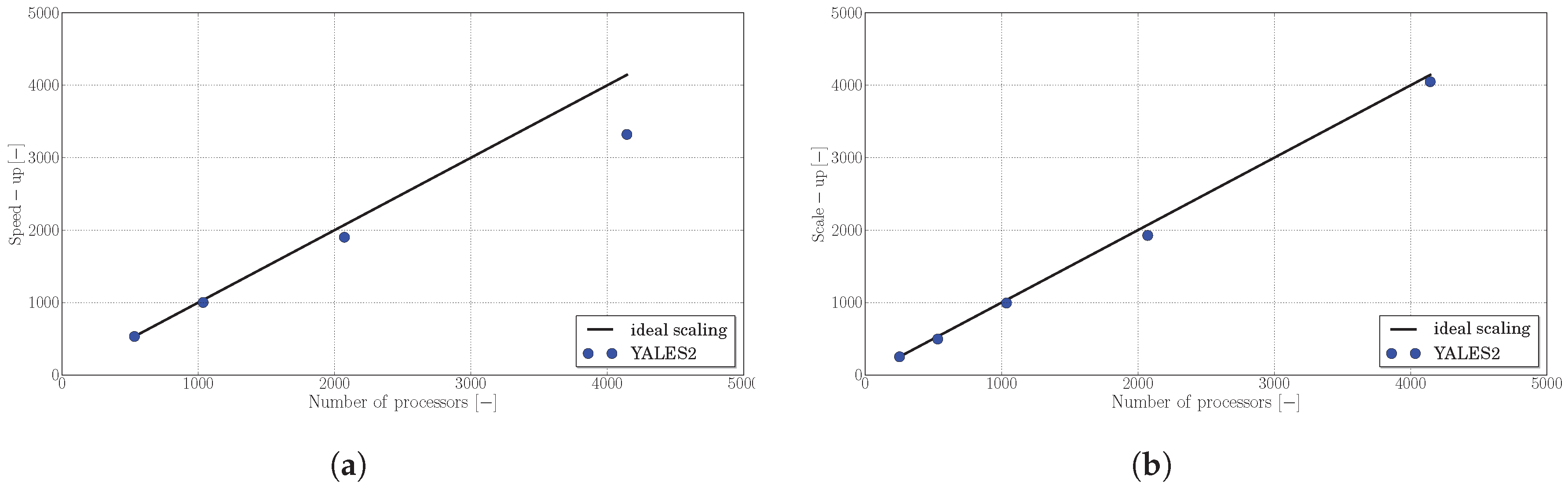
2.5. Performances and Parallelism

A critical point in the coupling between the gas and solid phase is the time advancement, as they can have very different time scales. The choice was made to sub-step the solid phase, of which time advancement is generally limited by the collision time step in dense fluidized beds, during a gas phase time step, which is itself governed by convective and diffusive time scales. The mean number of particle sub-steps observed during our simulations was approximately 3 for the refined mesh, 7 for the intermediate mesh and 16 for the coarse mesh (mesh details are described in the following section).
As the computation of the collision force requires a distance estimation for each particle pair a priori, solving Equations (40) and (41) can become critically time consuming. The work of Lubachevsky [25] provides an analysis of the linked-cell method to tackle this problem, which is the most commonly used method. The solution consists in the definition of a Cartesian grid superimposed on the grid mesh allowing each particle to search for its potential collision partners, as shown in Figure 5. First, each particle is located in one of the Cartesian grid cell. Then looping over the 8 surrounding cells plus the one where the particle stands ( 26 + 1 cells in 3D) provides a list of the closest particles, that are stored as potential collision partners. Eventually, during the computation of the collision force, only these particles are checked.
The linked-cell method is used even if the grid is Cartesian. This choice is justified by the fact that the cells of the detection grid should probably be (i) at least as big as the particle diameter (ii) as small as possible, in order to prevent too many neighboring particles from being detected. These requirements may be hard to guarantee if the Cartesian mesh is too coarse, or locally refined (which is one of the future aims of the code). For these reasons, a Cartesian grid is superimposed in any case.
Parallelism also requires special treatment for particles, as collision might occur between some of them although they don’t belong to the same processor domain. To cope with this requirement, a ghost particle method is used, which is also classical in CFD/DEM. Ghost particles are identified using a cell halo surrounding each processor domain as shown in Figure 6 for processor ranked # 1 in a cylindrical geometry discretized with an unstructured mesh. The particles belonging to the cell halo are exchanged between involved processors with the necessary data to compute collision force only by the mean of non-blocking Message Passing Interface (MPI) exchanges. The size of the cell halo is locally determined by the cell mesh size and particle diameter to avoid unwanted distant particles from being identified as ghost particles, which is not straightforward on unstructured meshes. On each processor, ghost particles are treated to be located as well on the afore mentioned Cartesian detection grid (see Figure 5).

2.6. Assessment of the Solver Performances

Assessments of the code global performances are first extracted from a canonical isothermal case, disregarding its physical relevance. This case consists of a cubic box meshed with tetrahedra. Particles are randomly seeded in the box, with a mean porosity of about 0.54 , and each tetrahedron contains roughly 11 particles. A fluid phase is present to account for the computational cost related to interpolation and projection steps. The particle timestep is chosen such that, ten particle timesteps are performed for each fluid timestep, which corresponds to a usual sub-stepping configuration. Code assessments are obtained from a single fluid timestep. All the tests were carried out on the regional supercomputer Myria of the CRIANN center (Centre Régional Informatique et d’Applications Numériques de Normandie, France), featuring a Intel Omni-Path interconnect. The processors used are Intel Broadwell 14 cores running at 2.4 GHz with 128 GB RAM (about 4 GB memory per core) for total peak power of 400 TFlop/s.
The speed-up is first obtained by running the same simulation on different numbers of cores, ranging from 532 (reference case) to 4144. Each simulation roughly gathers 38M tetrahedra and 410M particles. The reference CPU time t C P U r e f being associated with the temporal loop of the solver on N p r o c s r e f = 532 cores, the speed-up for a CPU time t C P U on N p r o c s is calculated by:
speed-up ( N p r o c s ) = N p r o c s r e f × t C P U r e f t C P U ,
and is illustrated on Figure 7a. The solver exhibits a good scalability up to 4144 cores, with a speed-up reaching 80 % of the ideal scaling.
Secondly, the scale-up of the solver is quantified by an evalutation of the performances at constant load per core on different numbers of cores, ranging from 252 (reference case) to 4144. The number of particles per core is about 99k, and the number of tetrahedra is about 9.1 k per core. The scale-up is given by:
scale-up ( N p r o c s ) = N p r o c s r e f × t C P U r e f N c r e f N c t C P U ,
where N c r e f and N c are the number of cells in the reference case and in the current case, respectively. The scale-up curve is represented on Figure 7b, which shows an excellent scaling.
Performances of the code are also assessed on an isothermal pressurized gas-fluidized bed carried out at the university of Birmingham [26]. The investigated case gathers 10M particles in a cylindrical domain meshed with 3.7 M tetrahedra. Here, the performances are extracted over 1 s of physical time after the stability of the bed fluidization has been assessed by monitoring both the bed height and the pressure loss across the system. Thus, this case deals with realistic conditions where the execution speed highly depends on the local physics (presence of dense or void zones), and where, the fluid and particle timesteps are recomputed throughout the simulation. The tests were carried out on the Curie supercomputer of the TGCC center (Trés Grand Centre de Calcul, France), featuring a InfiniBand QDR Full Fat Tree interconnect. The used nodes comprise two Intel Sandy Bridge octo-core processors running at 2.7 GHz with 64 GB RAM (about 4 GB per core).
The speed-up is obtained by running the simulation on various numbers of cores, ranging from 64 (reference case) to 1024 cores, and is illustrated on Figure 8. On the whole, the solver reaches 55 % of its ideal scaling value, which is acceptable given the high dispersion of the particles amongst the cores, causing their de-synchronizing.

3. Simulation Cases

3.1. Configuration and Meshes

In this work, CFD/DEM simulations of a fluidized bed, similar to that used in the experiments reported by Patil et al. [27], are performed. A sketch of the simulated configuration of the fluidized bed is shown in Figure 9 (left) including its dimensions. The bed contains inert glass particles fluidized by fresh nitrogen injected through the bottom of the bed at different gas flowrates. Physical properties of both gas and particles are summarized in Table 1. In the experiments, the bottom area of the bed was equipped with a small circular nozzle of 1.2 cm diameter, through which no gas was supplied during the experiments. In order to reproduce the effect of the switched nozzle as faithfully as possible, a zero gas flow was set through an area located at the center of the lower horizontal section of the bed. This area was considered as a wall for both gas and particles and is referred to as the bottom wall in the simulations. In the simulations, three different grid refinements were used and their characteristics are reported in Table 2, including that of the bottom wall retained for each mesh. As an example, a sketch of the intermediate mesh is illustrated in Figure 9 (right).

3.2. Description of the Simulation Cases

Several simulations based on different grid refinements, combined with different physical parameters, are investigated. In our modeling strategy, a friction coefficient, previously denoted as μ t a n in Section 2.2.1, is required to account for the tangential contact force during binary particle and particle-wall collisions. Since such a coefficient is not provided in the work of Patil et al. [27], we examined available values from the literature. As reported by Lorenz et al. [28], its value may depend on the state and history of the particle surfaces. The authors experimentally evaluated the friction coefficient, of glass particles having experienced a considerable time in granular flows, to 0.177 and 0.141 for inter-particle and particle-spent aluminum plate collisions, respectively. In the work of Goldschmidt et al. [29], values of 0.10 and 0.09 , as measured by Gorham et al. [30], were respectively used in the modeling of the particle-particle and the particle-wall frictional collisions in a dense gas-fluidized bed configuration. In Gorham et al., both the particles and the pseudo-2D bed were made of glass. In the following sections, we denote the particle-particle and the particle-wall friction coefficients as μ p and μ w , respectively. All the simulations are summarized in Table 3. A mesh sensitivity analysis, drawn from simulations C1, C2 and C3, for which μ p = μ w = 0.2 is assumed, is first presented. In a second step, various values of the friction coefficients, μ p and μ w , are investigated. This study refers to the sets of simulations C4 and C5, as shown in Table 3. The C4 simulations are performed using a constant value of μ p , with different values of μ w , whereas in the C5 simulations, the effect of μ p is investigated for a constant value of μ w . From these investigations, values for the friction coefficients are chosen by comparing numerical results of the volume fraction and the axial flux of the particulate phase with the available experimental measurements. Finally, additional Reynolds number and bed weight conditions are used as variable parameters for the simulations C6 and C7. It has to be mentioned that the inlet gas velocity, U f , given in Table 3 is the superficial velocity through the horizontal cross-sectional area of the bed (so, this area also includes the bottom wall). For each tested gas velocity, the corresponding particle Reynolds number, given as R e p = ρ U f d p / μ , is reported in the table, together with the Stokes number S t = ρ d p U f / ( 18 μ ) . It has to be noted that, the bulk Reynolds number based on the bed width is relatively high ( 5600 R e 8000 ). Therefore, for all the performed simulations, a turbulent viscosity based on Smagorinsky model is used. The additional parameter of interest is the restitution coefficient during particle-wall collisions, e w , which is considered equal to that of the particle-particle collisions, e n .

4. Results

Non-dimensional results are presented in this section. Since the lengths of the simulated configuration are different in all three directions a different length scale is defined in each direction. As a consequence, x -, y - and z -distances are divided by the bed width ( L = 0.08 m), the bed depth ( D = 0.015 m) and the bed height ( H = 0.25 m), respectively. The time scale is defined as t / ( d p / U f ) . The velocities are divided by the inlet gas velocity ( U f ) and the mass flowrates by the inlet gas mass flowrate ( ρ U f ). In order to characterize the bed hydrodynamics in an Eulerian fashion, the instantaneous fields of any Lagrangian variable, ψ p , are obtained by performing a spatial average over the grid cell. In addition, a 2D-behavior is considered for this fluidized bed configuration since the hydrodynamic variations in the depth direction are negligible. This can be observed in Figure 10, which displays the instantaneous particle volume fraction, α p , on different slices chosen at y / D = 0.2 (close to the back side), y / D = 0.5 (in the middle of the bed) and at y / D = 0.8 (close to the front side).
As an example, in Figure 11, profiles along the depth direction at the height z / H = 0.16 are also given for the time-averaged vertical velocity of the solid phase normalized by the inlet gas velocity ( U p , 3 ¯ / U f ). It can be observed that variations along the depth direction of such a quantity are not strong. Thus, two-dimensional variables are computed by averaging over the bed thickness (i.e., in the y-direction). In the present work, the 2D-variables corresponding to the computed field, < ψ p > , are denoted as < ψ p > x z . All the simulations are run for 20 s in order to reach a steady regime. In such a regime, particles and fluid hydrodynamic fields are statistically stationary and time-averaged quantities, < ψ k > ¯ , for which k denotes the gas (g) or the particulate (p) phase, may be computed for comparison with the experimental measurements.

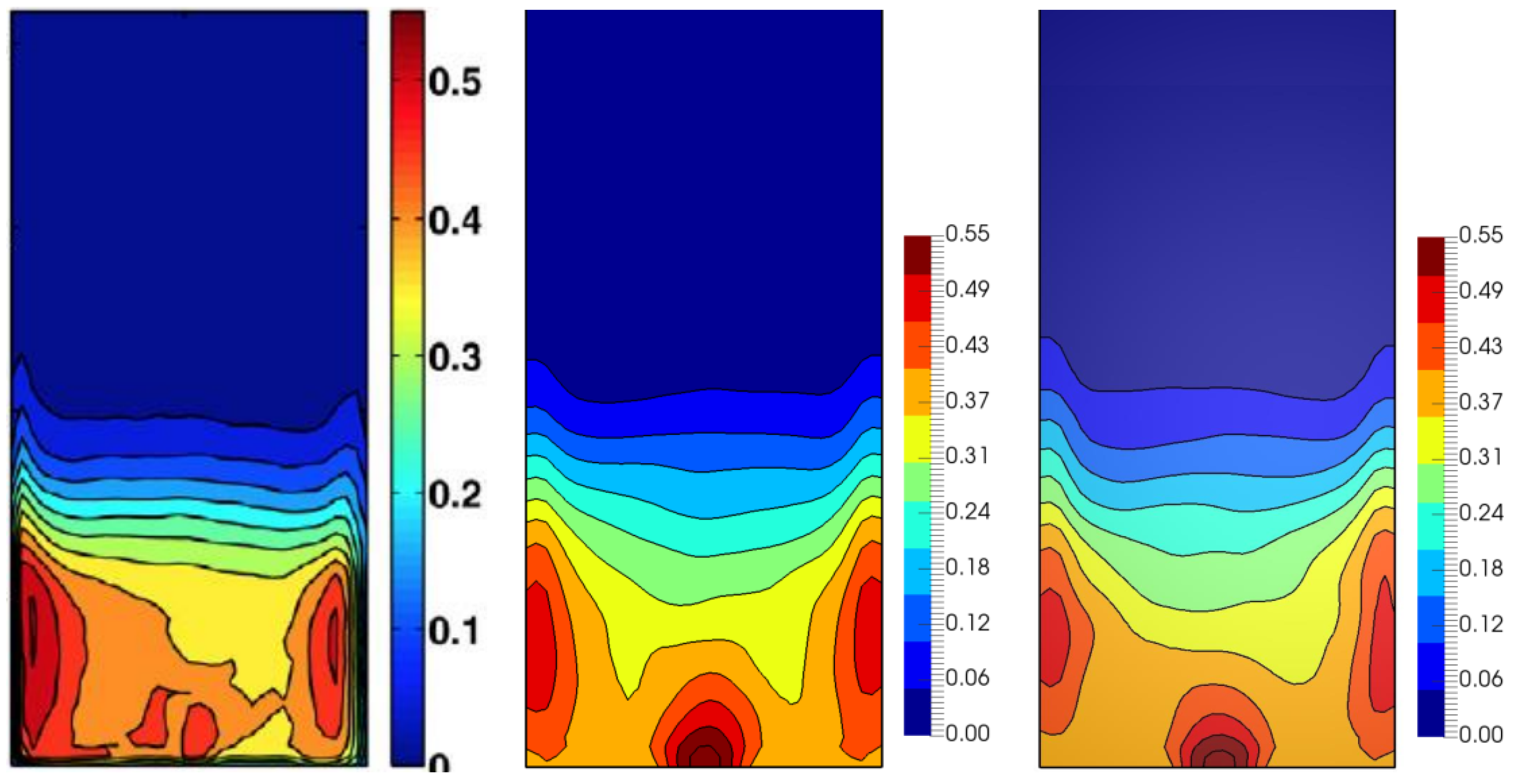
4.1. Effect of the Grid Refinement

In this section, the simulations C1, C2 and C3 are presented and discussed. The three simulations differ from each other by their mesh size, as shown in Table 2 and Table 3, and consequently by their filtering kernel length ( 4 Δ x ). However, because the kernel length is always larger than the particle diameter, the volume-averaged equations are well posed in the sense of Jackson [7]. Snapshots of the time-averaged fields concerning the volume fraction, < α p > x z ¯ , and the mass flux, < α p ρ p U p > x z ¯ , of the particulate phase are depicted in Figure 12 for the different grid refinements. Experimental results are also included in the right column. The simulations match quite well the experiments. The particle volume fraction exhibits high values (dense regions) close to the side and bottom walls and small values (dilute regions) in the center of the bed. However, the average height of the fluidized bed seems to be slightly overestimated by the simulations. The solid flux exhibits a macroscopic double mixing loop and, on average, the particles move upward at the center of the bed and downward close to the side walls. Comparison to experiments reveals that the center of the mixing loops, as predicted by the simulations, is located slightly higher than that experimentally observed. The three simulations indicate clearly that the mesh size affects the bed hydrodynamics prediction. The reason is that particles continuously interact with the gas flow through the drag and the pressure gradient forces, which then contributes to the particle dynamics evolution. Since the mesh resolution affects the hydrodynamics prediction of the gas phase, this consequently modifies the particle dynamics predictions. The upper panel of Figure 12, shows that the finest grid leads to the best predictions, as a result of an accurate resolution of the gas hydrodynamics. The high solid concentrations close to the side walls, as reported by the experiments, are reproduced with a relatively good accordance by the fine-grid simulation. Nevertheless, refining the mesh does not seem to have a significant effect on the height of these dense regions from the bottom of the bed, nor on the mean bed height. Indeed, refining the mesh “locally” improves the bed hydrodynamic predictions by improving the fluid velocity field around the solid particles, but it does not influence the predicted overall bed height. This latter is instead directly affected by the selected drag force model. This is the main reason why one-dimensional models are accurate regarding the prediction of the mean bed height, given a sufficiently appropriate drag model. The analysis of the time-averaged fields of the solid flux reveals, apart from the progressive intensification of these fields due to the increasing mesh resolution, that this latter did not influence the position of the observed double mixing loop.
Figure 13 shows profiles of the time-averaged vertical solid mass flux normalized by the gas mass flowrate, < α p ρ p U p , 3 > x z ¯ / ρ U f . The profiles are taken at the height z / H = 0.092 ( z = 2.3 cm) above the bottom of the bed, for which experimental data are available. We notice that the predictions are improved when the finest mesh is used, especially close to the side walls. However, at the center of the bed, the effect of the bottom wall on the axial solid flux is still poorly reproduced even when a finer mesh is used.
With the attempt to improve the numerical results, the wall boundary condition type on the gas phase was also investigated. Within the framework of Navier-Stokes equations, the wall boundary condition for the gas is no-slip. However, such a condition is questionable for averaged equations, as those employed in this work. In addition, the presence of the particles may profoundly modify the flow hydrodynamics. In the present work, slip and no-slip fine-grid simulation cases were run and compared to each other. The time-averaged results (not shown here) relative to the particulate phase were only very slightly affected by the selected wall condition of the gas phase. Such a behavior is inherent to inertial particles, as those simulated in the present work, for which the Stokes number is much greater than unity, as shown in Table 3.

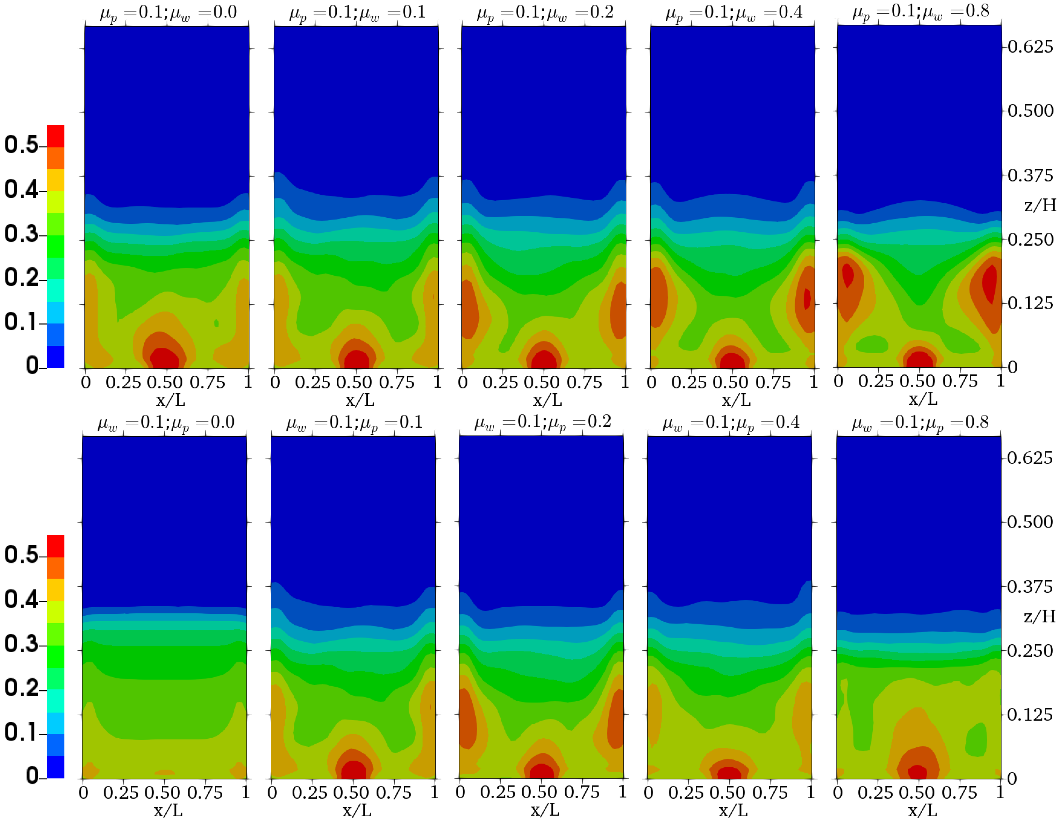
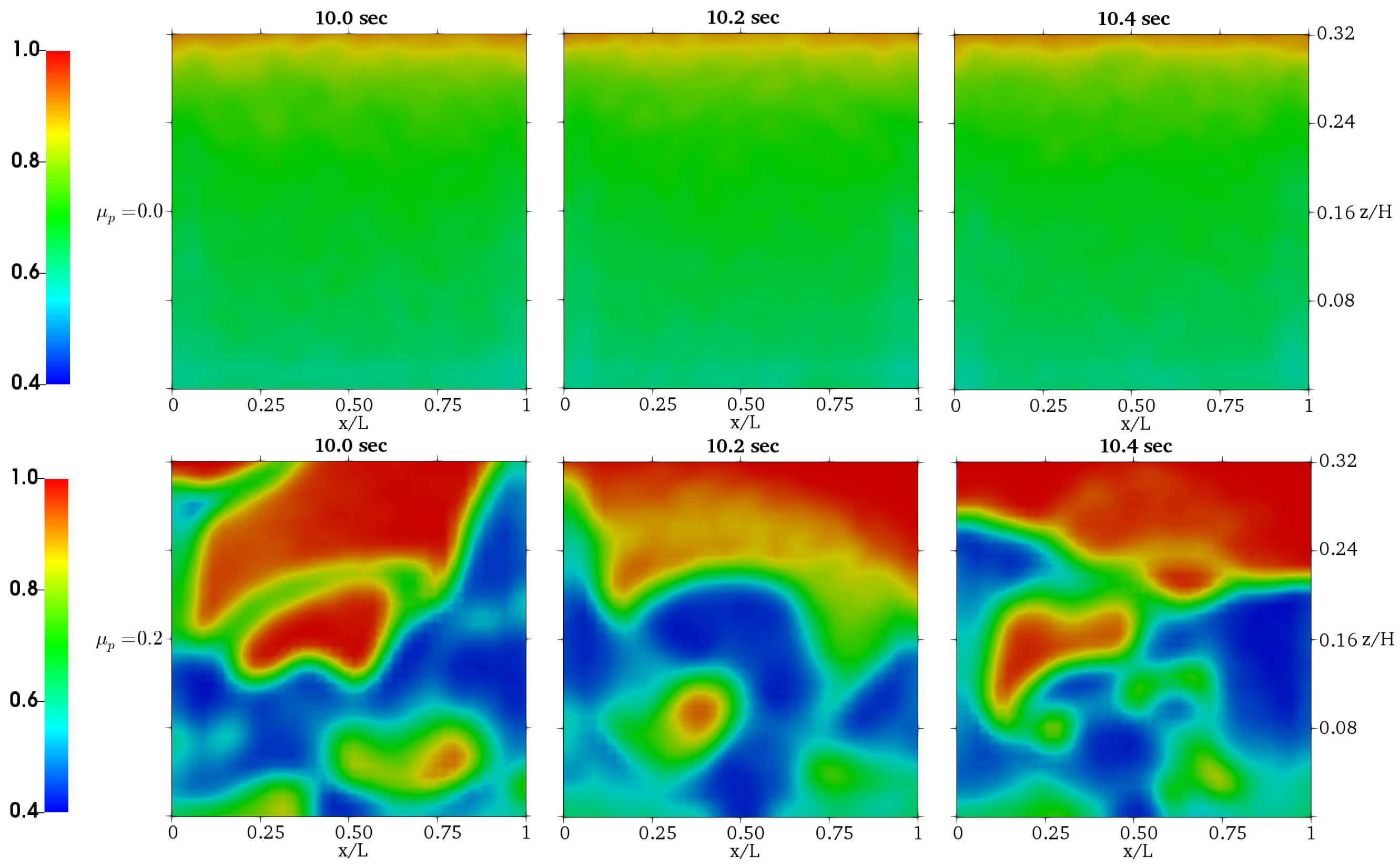
4.2. Investigation of the Frictional Effects

Effects of the inter-particle and the particle-wall friction coefficients on the bed hydrodynamics are here discussed. In the previous study, the computational time required by the fine-grid simulation was nearly twice higher than that of the intermediate-grid simulation. Therefore, the present study is carried out using the intermediate mesh.
The time-averaged fields concerning the particle volume fraction, as obtained from the sets of simulations C4 and C5 are shown in Figure 14. As previously mentioned, a dense region is observed close to the side and bottom walls, whereas, the center of the bed is characterized by a dilute solid concentration. In addition, the average height of the fluidized bed seems to decrease as the frictional effects become stronger. However, more subtle differences between the situations can be observed. The upper panel as obtained by the simulations C4, reveals that, for the same value of the particle friction coefficient, when the wall frictional effects become stronger, the dense regions become denser and larger near the side walls, while they are sligthly narrowing above the bottom wall. Results also show that such regions move slightly upwards as μ w increases. It has to be reminded that the influence of the wall friction coefficient is also exerted at the front and the back walls, but should be stronger in the confined parts of the bed, namely at the side walls, where the denser regions of the bed are observed. The bottom panel, obtained by the simulations C5, shows that, when μ p increases up to 0.2 , the bed hydrodynamics exhibit similar behavior as that observed when μ w varies and μ p is kept constant (simulations C4). Such results are in agreement with the work of Yang et al. [31], who showed the same trend of particle volume fraction distribution when μ p was increased from 0.05 to 0.15 , in their comparison study between two fluid model (TFM) and discrete particle model (DPM) simulations. However, unlike simulations C4, continuing to increase the particle-particle friction coefficient above the value of 0.2 in the simulations C5 resulted in decreasing the solid concentration near the side walls and increasing it above the bottom wall. The inter-particle friction acts on the whole bed volume and, as a consequence, high values of the inter-particle friction coefficient may considerably modify the bulk-bed hydrodynamic behavior. Finally, when the particle friction is not considered ( μ p = 0 for μ w = 0.1 ), a homogeneous fluidized bed is obtained, which is not the case for μ p 0 and μ w = 0 (simulations C4). These various bed behaviors inform about the effect of the particle friction on the bubble formation. As an exemple, snapshots of the instantaneous bed porosity (gas volume fraction), obtained at different instants by the simulations C5 for two values of μ p , are depicted in Figure 15. In the case of frictionless particles ( μ p = 0 ), no bubble formation occurs, whereas in the case of relatively frictional particles ( μ p = 0.2 ), a realistic bubble growth is observed. This is consistent with the work of Hoomans et al. [32], who showed the same bubble patterns in 2D-fluidized bed DPM simulations.
Time-averaged particle agitation energy, q p 2 , has been computed as q p 2 = u p , i u p , i ¯ , where u p , i = u p , i U p , i . In these expressions, u p , i and U p , i are the i t h components of the fluctuating and the mean particle velocities, respectively, with the mean particle velocity computed as U p , i = < u p , i > . The normalized results are shown in Figure 16 for the two sets of simulations. The first panel obtained from the set C4 shows that most of the particle agitation is produced at the approximate height z / h = 0.25 . This height corresponds to the average height of the dense bed ( α p > 0.2 ). Furthermore, it increases when friction at wall becomes stronger. Results of the simulations C5, as depicted in the bottom panel, show a decline, on average, of the particle agitation energy when the particle friction increases. In addition, some particle agitation is produced at the height z / h = 0.25 , similarly to what is observed in the C4 simulations. On the contrary, fewer amount of particle agitation is produced as the particle frictional effects become more significant. These results show that, for low friction between particles, the fluidized bed may be considerably heterogeneous when friction at wall is high and become homogeneous when friction between particles is strong. It has to be noted that, in all these simulations, the computed particle agitation energy in the upper part of the bed ( z / H 0.375 ), has a very low significance since, in this part, the particle volume fraction is nearly zero.
Figure 17 shows the time-averaged field of the solid mass flux for the two sets of simulations. From the visualizations, it appears that friction affects significantly the magnitude of the solid flux and the extent of the mixing loops. In some cases, it also affects their position from the bottom of the bed. As previously observed for the particle volume fraction distribution, the position of the centre of the double mixing loop moves upwards when μ w increases (upper pannel). This point is not straightforward when μ p is increased (bottom panel). However, qualitatively speaking, the magnitude of the solid flux exhibits a maximum for μ p = 0.2 in both sets of simulations.
A quantitative analysis of the solid flux may be performed via its vertical profiles at a given height of the bed. Profiles of the time-averaged normalized vertical solid mass flux are depicted in Figure 18a,b for the two sets of simulations. The profiles are taken at the height z / H = 0.092 ( z = 2.3 cm) above the bottom of the bed, for which experimental data are available. In all the simulations, two distinct parts for each profile can be observed. The first part corresponds to a nearly flat profile located in the region spanning the center of the bed and the second one is a sloped profile starting from the side walls. The expansion of one part to the detriment of the other depends on the values of the friction coefficients μ w and μ p . These coefficients also determine the maximum values of the upward and the downward mass fluxes in the flat and the sloped parts, respectively. The figures show that when μ w or μ p increases up to 0.2 , the downwarding flux increases and the upwarding flux, close to the center of the bed, decreases. This leads, at the same time, to a steeper slope of the solid mass flux profile in the sloped part and to a less broad flat part at the center of the bed. For a stronger friction, either at wall or between particles, larger sloped parts are still observed, but with less steep slopes, leading to the decrease of both the downwarding and the upwarding solid fluxes. Therefore, despite the differences observed concerning the volume fraction and the agitation energy of the particulate phase, simulations C4 and C5 predict similar characteristics (field and magnitude) of the solid mass flux. It is conjectured that, in this confined configuration, when the wall friction coefficient increases, the front and back walls may considerably contribute together with the side walls to propagate stronger wall frictional effects towards the bulk bed. This has already been shown in a previous CFD/DEM study of Li et al. [33] for bed thicknesses of 10 and 20 particle diameters in a bubbling fluidized bed. As a consequence, stronger wall friction may produce almost the same effect on the solid flux as that induced by the friction between particles.
Finally, comparison with the experimental measurements shows that, the case with μ p = μ w = 0.1 , is particularly interesting as it allows to reproduce the effect of the bottom wall on the axial solid flux (Figure 18) and to better predict the location of the solid mixing loops from the bottom of the bed (Figure 17 vs. experimental data from Figure 12). Nevertheless, the solid concentration close to the side walls seems to be slightly underestimated (Figure 14 vs. experimental data from Figure 12) and the solid loops more elongated than that experimentally reported. However, the predicted value of 0.1 for both the particle-particle and the particle-wall friction coefficients is noteworthy. In fact, the friction coefficient is a physical parameter that depends on the mechanical properties and the surface morphology of the solid particles, mainly Young’s modulus and the surface roughness. Its experimental measurement is also very sensitive to some environmental factors, such as wet or dry conditions and the exerted normal stress. For this reason, a wide range of values are reported in the literature for glass beads under various conditions. Values ranging from 0.139 to 0.464 have been determined by Ishibashi et al. [34] for 1.6 mm-sized particles under dry conditions and various normal forces. Sandeep and Senetakis [35] reported a unique value of 0.2 for glass particles of 2 mm diameter. Additionally, other values may also be found in the literature as this is previously discussed in Section 3.2. The predicted value of 0.1 in our simulations is deemed to be acceptable and it is in very good agreement with that used by Goldschmidt et al. [29] in their simulation of glass particles in a pseudo-2D dense fluidized bed.

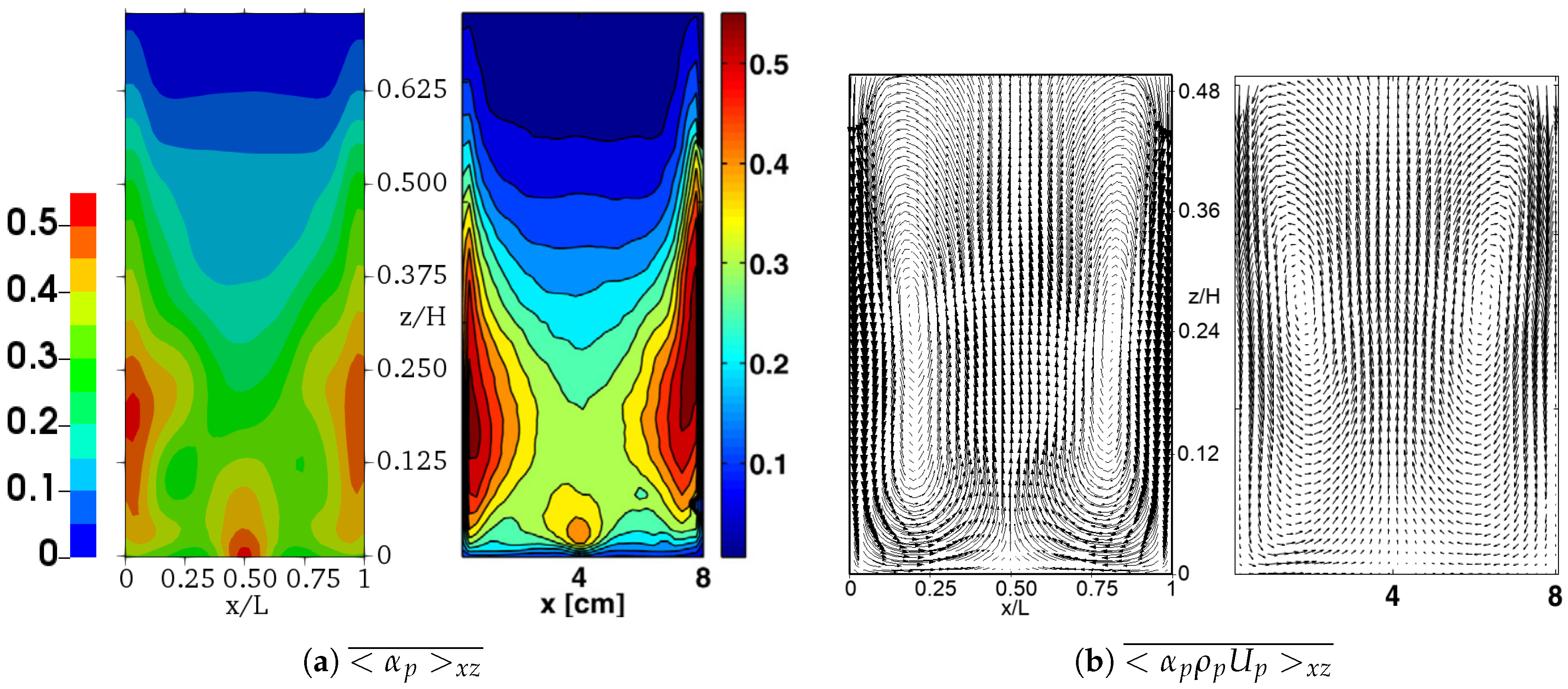
4.3. Application of the Results to Other Physical Configurations

In order to generalize the previous results to different physical configurations, other Reynolds number and bed weight conditions are investigated using the intermediate mesh. The same value of μ w and μ p and equal to 0.1 is used in the simulations since, as shown in Section 4.2, this leads to minor deviations from the experiments conducted for R e p = 70 . A gas no-slip condition at the wall is also retained. In the simulation C6, a superficial gas velocity of 1.71 m/s corresponding to R e p = 100 , as reported in Table 3, is imposed at the bottom of the bed. Predictions obtained by this simulation concerning the time-averaged fields of volume fraction and mass flux of the solid phase are reported in Figure 19a,b, respectively. Experimental measurements are also included for comparison purpose. One can see that the simulation reproduces very well the experimental solid distribution and the solid mass flux field. However, slight mismatches can be observed concerning the mean bed height and the position of the solid mixing loops. At the height z / H = 0.092 , numerical and experimental vertical mass fluxes are displayed on Figure 20. Globally, results are conveniently reproduced by the simulation and confirm the accuracy of the selection μ w = μ p = 0.1 .
Results of a fluidization experiment of 125 g of particles by nitogen injected at a velocity of 1.54 m/s, corresponding to R e p = 90 , have also been reported in Patil et al. [27]. This operating point is simulated in the present work (simulation C7) and results displayed in Figure 21a,b, together with the experimental data. Based on the investigations reported in Section 4.2, a value of the friction coefficient that allows to match as best as possible the experiments is retained. However, for all the simulations investigated so far, common deviations from the experiments are observed, namely concerning the mean bed height that appears overestimated, and the lateral solid recirculation zones which seem to be more elongated than that experimentally reported. The present simulation, using a higher bed weight, also does not sufficiently match the experiments, although the general pattern of the bed is globally well reproduced. Improvement of the numerical results should be achieved by, first, selecting an accurate drag law, which would allow to decrease the mean bed height, and then, by refining the mesh, which, as shown in Section 4.1, allows to accurately reproduce the solid concentration near the side walls.

5. Conclusions

In this work, a DEM/LES approach is used to simulate a confined fluidized bed configuration for several physical and numerical conditions. Results are compared with experimental data of [27]. This study shows that, compared with the experimental measurements, predictions regarding the volume fraction and the mass flux of the particulate phase, obtained from the fine grid, are slightly better than that of the coarse and the intermediate grids. This slight improvement is attributed to a better prediction of the gas-particle interactions through the drag and the pressure gradient forces. The present work is also dedicated to frictional effects between particles and between particles and walls on the bed hydrodynamics behavior. It is shown that, increasing either the coefficient of the inter-particle friction or that of the particle-wall friction, the average bed height decreases and the bubble formation is enhanced. At low friction between particles, increasing the wall friction coefficient leads to similar solid circulation patterns (fields and magnitudes) as in the simulations with increasing friction between particles. Thus, it is conjectured that, in such confined 2D-configuration, when the wall friction coefficient increases, the friction of the front and back walls may have a significant impact on the inner-flow hydrodynamics of the fluidized bed. This finally may lead to the same bed hydrodynamics behavior as that observed when the friction coefficient between particles increases. Nevertheless, this point has to be further investigated. Indeed, to clearly understand the contribution of the friction at the front and back walls, simulations with various bed thicknesses combined with different values of the friction coefficients have to be performed. Additional simulations, performed at higher Reynolds numbers and/or other bed weights, showed globally good agreement with the experiments, reproducing almost similar particle volume fraction and solid circulation patterns as the experiments. However, deviations from the experiments concerning the average height of the dense bed is still exhibited in all the simulations. This could be further enhanced by studying other modeling features, such as the drag law.

Author Contributions

Investigation, Z.H.; Methodology, Y.D.; Supervision, J.-L.P., R.B., G.L. and V.M.

Funding

Computations were performed on the IFPEN supercomputer ENER110 and on the supercomputer CURIE under the project GENCI A0032B07345. The ENER110 and GENCI supercomputers teams are gratefully acknowledged. This work is done in the frame of the MORE4LESS project funded by the French National Research Agency.

Acknowledgments

Olivier Simonin at Institut National Polytechnique de Toulouse (France) is gratefully acknowledged for fruitful discussions throughout this work.

Conflicts of Interest

The authors declare no conflict of interest. The funders had no role in the design of the study; in the collection, analyses, or interpretation of data; in the writing of the manuscript, or in the decision to publish the results.

Abbreviations

The following abbreviations are used in this manuscript:
CFLCourant-Friedrichs-Lewy
DEMDiscrete Element Method
DPCGDeflated Preconditioned Conjugate Gradient
DPMDiscrete Particle Model
DNSDirect Numerical Simulation
LESLarge-Eddy Simulation
MPIMessage Passing Interface
PCMParticle Centroid Method
RKRunge–Kutta
SCSurrounding Cell
TFMTwo Fluid Model
BNBlue Nodes
GNGreen Nodes
RNRed Nodes

Appendix A. Influence of LES Model on the Numerical Results

In order to clearly assess the influence of the LES model on the numerical simulations we performed additional simulations with and without LES model. The physical and numerical parameters corresponds to case C6 in Table 3. Figure A1 shows that there almost no difference between the case using a LES model and the case with no model. The closure law for small scale structures have a weak impact on the flow which means that the dissipation is mainly governed by the large scale structure and by particle-particle friction.
Figure A1. Time-averaged particle volume fraction. (Left): Experimental results, (middle): numerical results using Smagorinsky model, (right): numerical results without Smagorinsky model.
Fluids 04 00051 g0a1

References

  1. Tenneti, S.; Subramaniam, S. Particle-resolved direct numerical simulation for gas-solid flow model development. Annu. Rev. Fluid Mech. 2014, 46, 199–230. [Google Scholar] [CrossRef]
  2. Pepiot, P.; Desjardins, O. Numerical analysis of the dynamics of two-and three-dimensional fluidized bed reactors using an Euler–Lagrange approach. Powder Technol. 2012, 220, 104–121. [Google Scholar] [CrossRef]
  3. Alder, B.J.; Wainwright, T. Phase transition for a hard sphere system. J. Chem. Phys. 1957, 27, 1208–1209. [Google Scholar] [CrossRef]
  4. Cleary, P.W. Industrial particle flow modelling using discrete element method. Eng. Comput. 2009, 26, 698–743. [Google Scholar] [CrossRef]
  5. Deen, N.G.; Annaland, M.V.S.; Van der Hoef, M.A.; Kuipers, J.A.M. Review of discrete particle modeling of fluidized beds. Chem. Eng. Sci. 2007, 62, 28–44. [Google Scholar] [CrossRef]
  6. Sundaresan, S. Reflections on mathematical models and simulation of gas-particle flows. In Proceedings of the 10th International Conference on Circulating Fluidized Beds and Fluidization Technology; Knowlton, T., PSRI, Eds.; ECI Symposium Series; Princeton University: Princeton, NJ, USA, 2011. [Google Scholar]
  7. Jackson, R. The Dynamics of Fluidized Particles; Cambridge University Press: Cambridge, UK, 2000. [Google Scholar]
  8. Capecelatro, J.; Desjardins, O. An Euler–Lagrange strategy for simulating particle-laden flows. J. Comput. Phys. 2013, 238, 1–31. [Google Scholar] [CrossRef]
  9. Moureau, V.; Domingo, P.; Vervisch, L. Design of a massively parallel CFD code for complex geometries. C. R. Mécanique 2011, 339, 141–148. [Google Scholar] [CrossRef]
  10. Chorin, A.J. Numerical solution of the Navier-Stokes equations. Math. Comput. 1968, 22, 745–762. [Google Scholar] [CrossRef]
  11. Pierce, C.D.; Moin, P. Progress-variable approach for large-eddy simulation of non-premixed turbulent combustion. J. Fluid Mech. 2004, 504, 73–97. [Google Scholar] [CrossRef]
  12. Moureau, V.; Domingo, P.; Vervisch, L. From large-eddy simulation to direct numerical simulation of a lean premixed swirl flame: Filtered laminar flame-pdf modeling. Combust. Flame 2011, 158, 1340–1357. [Google Scholar] [CrossRef]
  13. Smagorinsky, J. General circulation experiments with the primitive equations: I. The basic experiment. Mon. Weather Rev. 1963, 91, 99–164. [Google Scholar] [CrossRef]
  14. Germano, M.; Piomelli, U.; Moin, P.; Cabot, W.H. A dynamic subgrid-scale eddy viscosity model. Phys. Fluids A Fluid Dyn. 1991, 3, 1760–1765. [Google Scholar] [CrossRef]
  15. Lilly, D.K. A proposed modification of the Germano subgrid-scale closure method. Phys. Fluids A Fluid Dyn. 1992, 4, 633–635. [Google Scholar] [CrossRef]
  16. Cundall, P.A.; Strack, O.D. A discrete numerical model for granular assemblies. Géotechnique 1979, 29, 47–65. [Google Scholar] [CrossRef]
  17. Ergun, S. Fluid Flow through Packed Columns. J. Chem. Eng. Prog. 1952, 48, 89–94. [Google Scholar]
  18. Wen, C.Y.; Yu, Y.H. A generalized method for predicting the minimum fluidization velocity. AlChE J. 1966, 12, 610–612. [Google Scholar] [CrossRef]
  19. Huilin, L.; Gidaspow, D. Hydrodynamics of binary fluidization in a riser: CFD simulation using two granular temperatures. Chem. Eng. Sci. 2003, 58, 3777–3792. [Google Scholar] [CrossRef]
  20. Sun, R.; Xiao, H. Diffusion-based coarse graining in hybrid continuum–discrete solvers: Applications in CFD-DEM. Int. J. Multiph. Flow 2015, 72, 233–247. [Google Scholar] [CrossRef]
  21. Mendez, S.; Gibaud, E.; Nicoud, F. An unstructured solver for simulations of deformable particles in flows at arbitrary Reynolds numbers. J. Comput. Phys. 2014, 256, 465–483. [Google Scholar] [CrossRef]
  22. Kraushaar, M. Application of the Compressible and Low-Mach Number Approaches to Large-Eddy Simulation of Turbulent Flows in Aero-Engines. Ph.D. Thesis, Institut National Polytechnique de Toulouse, Toulouse, France, 2011. [Google Scholar]
  23. Van der Vorst, H.A. Parallel iterative solution methods for linear systems arising from discretized pde’s. In Special Course on Parallel Computing in CFD; France Workshop Lecture Notes; 1995; Available online: https://www.semanticscholar.org/paper/Parallel-Iterative-Solution-Methods-for-Linear-from-Vorst/907dfb316057751b85e8620cf02d4fecb9ed731d (accessed on 12 February 2019).
  24. Van der Hoef, M.A.; Ye, M.; van Sint Annaland, M.; Andrews, A.T.; Sundaresan, S.; Kuipers, J.A.M. Multiscale modeling of gas-fluidized beds. Adv. Chem. Eng. 2006, 31, 65–149. [Google Scholar]
  25. Lubachevsky, B.D. How to simulate billiards and similar systems. J. Comput. Phys. 1991, 94, 255–283. [Google Scholar] [CrossRef]
  26. Fede, P.; Moula, G.; Ingram, A.; Dumas, T.; Simonin, O. 3D Numerical simulation and PEPT experimental investigation of pressurized gas-solid fluidized bed hydrodynamic. Presented at the ASME 2009 Fluids Engineering Division Summer Meeting, Vail, CO, USA, 2–6 August 2009. [Google Scholar]
  27. Patil, A.V.; Peters, E.A.J.F.; Kuipers, J.A.M. Comparison of CFD-DEM heat transfer simulations with infrared/visual measurements. Chem. Eng. J. 2015, 277, 388–401. [Google Scholar] [CrossRef]
  28. Lorenz, A.; Tuozzolo, C.; Louge, M.Y. Measurements of impact properties of small, nearly spherical particles. Exp. Mech. 1997, 37, 292–298. [Google Scholar] [CrossRef]
  29. Goldschmidt, M.J.V.; Beetstra, R.; Kuipers, J.A.M. Hydrodynamic modelling of dense gas-fluidised beds: Comparison and validation of 3D discrete particle and continuum models. Powder Technol. 2004, 142, 23–47. [Google Scholar] [CrossRef]
  30. Gorham, D.A.; Kharaz, A.H. Results of particle impact tests. In Impact Research Group Report IRG 13; The Open University: Milton Keynes, UK, 1999. [Google Scholar]
  31. Yang, L.; Padding, J.J.; Kuipers, J.H. Investigation of collisional parameters for rough spheres in fluidized beds. Powder Technol. 2017, 316, 256–264. [Google Scholar] [CrossRef]
  32. Hoomans, B.P.B.; Kuipers, J.A.M.; Briels, W.J.; van Swaaij, W.P.M. Discrete particle simulation of bubble and slug formation in a two-dimensional gas-fluidised bed: A hard-sphere approach. Chem. Eng. Sci. 1996, 51, 99–118. [Google Scholar] [CrossRef]
  33. Li, T.; Gopalakrishnan, P.; Garg, R.; Shahnam, M. CFD–DEM study of effect of bed thickness for bubbling fluidized beds. Particuology 2012, 10, 532–541. [Google Scholar] [CrossRef]
  34. Ishibashi, I.; Perry, C., III; Agarwal, T.K. Experimental determination of contact friction for spherical glass particles. Soils Found. 1994, 34, 79–84. [Google Scholar] [CrossRef]
  35. Sandeep, C.S.; Senetakis, K. Effect of Young’s modulus and surface roughness on the inter-particle friction of granular materials. Materials 2018, 11, 217. [Google Scholar] [CrossRef]
Figure 1. 2D representation of a particle p located in a triangular cell ( Fluids 04 00051 i001) moving towards a neighboring cell ( Fluids 04 00051 i002). Fluids 04 00051 i003: mesh nodes. Fluids 04 00051 i004: contour of node 3 control volume. ω p , i : interpolation weight of particle p on node i.
Fluids 04 00051 g001
Figure 2. On the left: 2D representation of an unstructured mesh. Fluids 04 00051 i003: mesh nodes. The control volumes of nodes i 1 ( Fluids 04 00051 i001), i 2 ( Fluids 04 00051 i005), i 3 ( Fluids 04 00051 i006), i 4 ( Fluids 04 00051 i007), i 5 ( Fluids 04 00051 i008), i 6 ( Fluids 04 00051 i009), i 7 ( Fluids 04 00051 i002) are shown. The control volume of node i 1 is composed of surfaces S 23 , S 34 , S 45 , S 56 , S 67 and S 72 . On the right: 3D representation of a regular Cartesian mesh part. Fluids 04 00051 i003: node i 1 . Fluids 04 00051 i010: nodes at faces’ center. Fluids 04 00051 i011: nodes at edges’ center. Fluids 04 00051 i012: nodes at corners.
Fluids 04 00051 g002
Figure 3. The simple test consists of a single particle colliding a wall in the normal direction. Only the collision force is accounted for and the parameters used for the resolution are visible on the right side. The contact starts at t = 0 .
Fluids 04 00051 g003
Figure 4. Non-dimensional overlap (a) and velocity (b) as a function of the non-dimensional time during the contact presented in Figure 3. Comparison between analytical method ( Fluids 04 00051 i013), Euler method with t p = T C / 80 ( Fluids 04 00051 i014) and RK2 method with t p = T C / 6 ( Fluids 04 00051 i015).
Fluids 04 00051 g004
Figure 5. Linked-cell method. Fluids 04 00051 i003: mesh nodes. Fluids 04 00051 i013: superimposed Cartesian grid. The particle of interest is noted p in the central cell ( Fluids 04 00051 i001). The particles of which center belongs to this cell or one of the surrounding ones ( Fluids 04 00051 i002) are stored as potential collision partners of particle p.
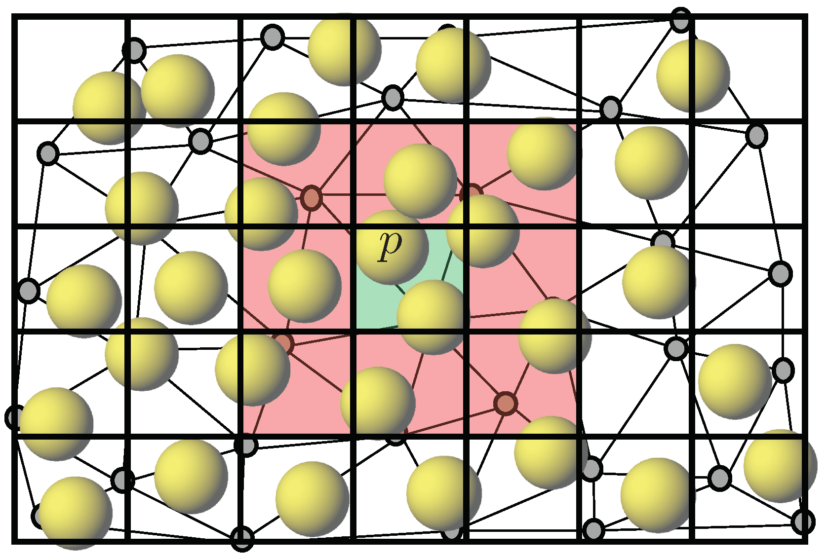
Fluids 04 00051 g005
Figure 6. Ghost particle method principle shown for a part of a cylindrical domain. The different processor domains are colored accordingly. The processor of interest is ranked # 1 ( Fluids 04 00051 i016) and its closest neighbors are ranked # 2 , # 3 , # 4 , # 5 and # 6 . A particle entering the white cell halo around # 1 will be sent to # 1 as a ghost particle by the processor it belongs to.
Fluids 04 00051 g006
Figure 7. Speed-up (a) and scale-up (b) curves extracted from the canonical case.
Fluids 04 00051 g007
Figure 8. Speed-up curve obtained on the Birmingham fluidized bed.
Fluids 04 00051 g008
Figure 9. Sketches of the simulated configuration (left) and of the intermediate mesh (right).
Fluids 04 00051 g009
Figure 10. Instantaneous particle volume fraction on different slices of the bed. Simulation C2, dimensionless time t / ( d p / U f ) = 12,000, μ w = μ p = 0.2 , R e p = 70 and bed weight 75 g.
Fluids 04 00051 g010
Figure 11. Profiles of the time-averaged normalized vertical velocity of the particulate phase ( U p , 3 ¯ / U f ) at different locations x / L . Simulation C2, μ w = μ p = 0.2 , R e p = 70 and bed weight 75 g.
Fluids 04 00051 g011
Figure 12. Numerical predictions of the time-averaged fields of the volume fraction, < α p > x z ¯ , (upper panel) and the mass flux, < α p ρ p U p > x z ¯ , (bottom panel) of the solid phase. From left to right, increasing grid refinement with μ w = μ p = 0.2 , and comparison with the experiments (right column). R e p = 70 and bed weight 75 g.
Fluids 04 00051 g012
Figure 13. Time-averaged normalized vertical mass flux of the solid phase, < α p ρ p U p , 3 > x z ¯ / ρ U f , at the height z / H = 0.092 above the bottom bed, for different grid refinements. μ w = μ p = 0.2 , R e p = 70 and bed weight 75 g.
Fluids 04 00051 g013
Figure 14. Time-averaged particle volume fraction, < α p > x z ¯ , for different values of the particle–wall μ w and the particle–particle μ p friction coefficients. Upper panel: constant μ p and different μ w . Bottom panel: constant μ w and different μ p . R e p = 70 and bed weight 75 g.
Fluids 04 00051 g014
Figure 15. Instantaneous gas volume fraction, with μ w = 0.1 . Upper panel: μ p = 0 . Bottom panel: μ p = 0.2 . R e p = 70 and bed weight 75 g.
Fluids 04 00051 g015
Figure 16. Time-averaged dimensionless particle agitation energy, q p 2 / U f 2 for different values of the particle-wall μ w and the particle-particle μ p friction coefficients. Upper panel: constant μ p and different μ w . Bottom panel: constant μ w and different μ p . R e p = 70 and bed weight 75 g.
Fluids 04 00051 g016
Figure 17. Time-averaged solid mass flux, < α p ρ p U p > x z ¯ , for different values of the particle–wall μ w and the particle–particle μ p friction coefficients. Upper panel: constant μ p and different μ w . Bottom panel: constant μ w and different μ p . R e p = 70 and bed weight 75 g.
Fluids 04 00051 g017
Figure 18. Time-averaged vertical solid mass flux normalized by the gas mass flow rate, < α p ρ p U p , 3 > x z ¯ / ρ U f , for different values of the particle–wall and particle–particle friction coefficients, and comparison with experiments. R e p = 70 and bed weight 75 g.
Fluids 04 00051 g018
Figure 19. Numerical (a) against experimental (b) time-averaged fields of the volume fraction and the mass flux of the solid phase. R e p = 100 and bed weight 75 g. In the simulation, μ w = μ p = 0.1 .
Fluids 04 00051 g019
Figure 20. Numerical against experimental time-averaged vertical mass flux, < α p ρ p U p , 3 > x z ¯ / ρ U f , of the solid at the height z / H = 0.092 above the bottom of the bed. R e p = 100 and bed weight 75 g. In the simulation, μ w = μ p = 0.1 .
Fluids 04 00051 g020
Figure 21. Numerical (a) againt experimental (b) time-averaged fields of the volume fraction and the mass flux of the solid phase. R e p = 90 and bed weight 125 g. In the simulation, μ w = μ p = 0.1 .
Fluids 04 00051 g021
Table 1. Gas and particle properties [27].
Gas Properties (at 20 C)
Density, ρ 1.165 kg/m 3
Viscosity, μ 2 × 10 5 Pa·s
Particle Properties
Mean diameter, d p 1 mm
Density, ρ p 2500 kg/m 3
Norm. coef. of rest., e n 0.97
Solid/gas density ratio, ρ p / ρ 2146
Table 2. Mesh characteristics.
MeshNumber of CellsBottom WallMesh Size/Particle Diameter Ratio
N x N y N z Total N x N y Δ x / d p Δ y / d p Δ z / d p
Coarse173552805334.7065.0004.545
Intermediate35611023,100542.2862.5002.273
Fine7012220184,8001081.1431.2501.136
Table 3. Simulation cases with the selected physical and numerical parameters.
SimulationBed U f (m/s) Friction CoefficientsMesh
CasesMass (g)at 20  C Re p St μ p μ w
C175 1.20 70∼4 μ p = μ w = 0.2 Coarse
C2Intermediate
C3Fine
C475 1.20 70∼4 0.1 0.0 Intermediate
0.2
0.2
0.4
0.8
C575 1.20 70∼4 0.0 0.1 Intermediate
0.2
0.2
0.4
0.8
C675 1.71 100∼5.5 μ p = μ w = 0.1 Intermediate
C7125 1.54 90∼ 5 μ p = μ w = 0.1 Intermediate

