Efficiently Generating Mixing by Combining Differing Small Amplitude Helical Geometries

Abstract

Helical geometries have been used in recent years to form cardiovascular prostheses such as stents and shunts. The helical geometry has been found to induce swirling flow, promoting in-plane mixing. This is hypothesised to reduce the formation of thrombosis and neo-intimal hyperplasia, in turn improving device patency and reducing re-implantation rates. In this paper we investigate whether joining together two helical geometries, of differing helical radii, in a repeating sequence, can produce significant gains in mixing effectiveness, by embodying a ‘streamline crossing’ flow environment. Since the computational cost of calculating particle trajectories over extended domains is high, in this work we devised a procedure for efficiently exploring the large parameter space of possible geometry combinations. Velocity fields for the single geometries were first obtained using the spectral/hp element method. These were then discontinuously concatenated, in series, for the particle tracking based mixing analysis of the combined geometry. Full computations of the most promising combined geometries were then performed. Mixing efficiency was evaluated quantitatively using Poincaré sections, particle residence time data, and information entropy. Excellent agreement was found between the idealised (concatenated flow field) and the full simulations of mixing performance, revealing that a strict discontinuity between velocity fields is not required for mixing enhancement, via streamline crossing, to occur. Optimal mixing was found to occur for the combination $R=0.2D$ and $R=0.5D$, producing a $70\%$ increase in mixing, compared with standard single helical designs. The findings of this work point to the benefits of swirl disruption and suggest concatenation as an efficient means to determine optimal configurations of repeating geometries for future designs of vascular prostheses.

1. Introduction

Helical pipe based geometries have been previously investigated for their ability to generate swirling flow and in-plane mixing [1,2]. These flow attributes are thought to be beneficial in preventing the formation of thrombosis within vascular prostheses, as well as reducing neo-intimal hyperplasia near to the graft anastomoses. Though internal mammal artery grafts are achieving patency rates of 90–95% after 15 years, saphenous vein grafts have patency rates of only roughly $50\%$ after 10 years [3]. Due to a range of factors including an ageing population, increased incidence of re-operations, and pre-existing vascular diseases, it is estimated that up to 20% of patients are unsuitable for autologous grafting [4]. Therefore improvements in prosthetic graft patency are highly desirable.

Similarly, as of 2009 the one and two-year cumulative patency rates for expanded polytetrafluoroethylene (ePTFE) vascular access grafts are 59–90% and 47–85% respectively, in the arm, and 41–68% and 26–43% in the thigh, respectively [5]. Finally, even though drug-eluting stents have reduced the stent restenosis rates to approximately 2.6–10.1%, [6], they are still susceptible to stent thrombosis due to delayed re-endothelialisation [7]. Taken together there remains significant potential for helical geometry based technologies to improve clinical outcomes for these interventions, particularly if combined with advances in bio-materials.

Following the observation that arterial geometries tend to possess both curvature and torsion, creating a physiologically favourable flow environment [8], Caro et al. [2] proposed that small amplitude helical pipes would induce a similar swirling flow and therefore could be used to improve the patency of both bypass grafts and arterio-venous (A-V) shunts. A preliminary clinical study by Huijbregts et al. [9] showed that helical pipes used as arterio-venous access grafts (or A-V shunts) for dialysis yielded some improvements in assisted primary and secondary patency, but that reductions in helical geometry observed via angiography may have reduced the potential benefits. The authors previously performed a numerical investigation of the flow in these small amplitude helical pipes [1], showing that mixing was generated by a double-vortex structure, which was maximised when the structure was approximately symmetric at a helical radius, R, equal to $0.25D$, where D is the pipe internal diameter. Increasing helical amplitude or radius beyond this yielded only marginal improvements in mixing, but for disproportionately higher pressure losses. The properties of this vortex structure in helical pipes were harnessed in a helical bioreactor proposed by Van Doormaal and Ethier, as it allowed for the possibility of independently controlling shear stress environment and particle residence times [10].

Various studies have performed computational investigations of helical pipe based geometries to understand the flow physics both within and downstream of the graft. Coppola and Caro [11,12] investigated the potential for mixing induced by the helical geometry to improve the flux of oxygen to the vessel wall. Lee et al. [13] investigated the dependence of wall shear stress and vortical structure on curvature and torsion. Ha et al. [14] presented a possible optimised helical design for use in the presence of stenosis, using the degree of swirl as the design optimisation target. Zheng et al. studied the effect of Dean number and geometry under steady flow conditions [15], and unsteady flow in a single geometry [16]. Van-Canneyt et al. [17] compared the flow within conventional and helical grafts when used in an A-V shunt configuration, examining flow parameters both within the graft and at the anastomoses, finding that a shorter pitch length is potentially beneficial from a physiological point of view.

An alternative approach to generating a swirling flow was proposed by Stonebridge et al. [18], embodied in the Spiral Flow graft product, which uses a helical ridge on the interior wall of a straight pipe rather than displacing the entire boundary in a helical fashion. First-in-man tests of this device used for infrainguinal bypass grafting showed $86\%$, and $73\%$, 12-month patency rates for above-the-knee, and below-the-knee, grafts respectively [18]. This technology has also been implemented as an A-V shunt, where a study of 48 cases showed promising improvements in patency for the Spiral Flow graft after one year, compared to straight ePTFE and heparin-bonded grafts [19]. The spiral ridge concept was extended by Kabinejadian et al. [20,21], who combined a helical ridge and helical pipe boundary, finding that this combination produced greater swirling flow in the graft anastomosis than either concept implemented alone.

Helical geometries have also been applied to the design of cardiovascular stents to create a more physiologically similar flow environment within the stented region [22], with the added benefit that a helical geometry may also be less prone to kinking both during, and following, implantation. Shinke et al. [23] tested a helical stent developed by Veryan Medical, Ltd in a healthy porcine model of the carotid arteries finding that though neointimial morphometry was similar to a straight stent, there was a significant reduction in intimal thickening with the helical stents, which was attributed to the swirling flow through the stent, as observed by duplex Doppler ultrasound. These stents subsequently underwent a clinical trial for use in the femoropopliteal artery as an intervention for peripheral arterial disease, finding that after two years a helical centreline stent had an equal therapeutic effect to a standard design, but showed greater device patency [24,25].

The vast majority of these studies have considered standard helical geometries with spatially constant geometric parameters. However, Rajbanshi and Ghatak [26] proposed a novel triple helical channel, which comprised three circular cross-section helical pipes joined together in parallel along a common surface in the axial direction, as a means of generating enhanced mixing. This configuration is particularly well suited to industrial applications that require the mixing of three separate liquids under low Reynolds number flow conditions, however it is less suited to use as a vascular prosthesis.

Though a quantitative link between the degree of fluid mixing and the degree of prevention of thrombosis is not currently established, there are two main aspects of mixing, and specifically mixing in helical pipe flows, that are hypothesised here to confer benefits regarding thrombosis prevention. The first is that mixing reduces mean residence time within the pipe and reduces extrema of residence times [1]. In-plane mixing more specifically moves particles away from the wall into the core, thus reducing near-wall residence times. Ramstack et al. [27] defined a platelet activation parameter that is the product of shear rate and time. Therefore in the presence of in-plane mixing, fewer platelets should experience a damaging shear rate for a long enough time to reach the activation value of 1000. Fewer activated platelets should thus reduce the amount of, and/or rate of production of, thrombosis. Secondly, due to the torsion of helical geometries, there is an angular offset between peak axial velocity (strongly correlated with the location of high wall shear stress) and the region of secondary flow directing particles to the wall. This is in contrast to Dean flow in which these two regions of the flow align exactly. A helical pipe flow therefore reduces the near-wall residence time of particles experiencing the highest shear stresses.

In this paper it is proposed that mixing in helical pipes can be enhanced by joining together pipes of differing helical radius in a series configuration that is suited to biomedical applications. This configuration embodies the concept of ‘streamline crossing’, which is known to generate chaotic particle trajectories [28] and hence good fluid mixing. This paper presents a numerical investigation of these geometries in order to understand this mixing behaviour, and is organised as follows: Section 2 provides more detail on the flow physics that govern this design concept, drawing comparison with the work of Jones et al. [28]. Section 3 then outlines the selection of geometric parameters for investigation, as well as the methods for solving the Navier-Stokes equations and performing the analysis of the mixing behaviour. In Section 4 results are shown first for an idealised prediction of the mixing performance, after which the most promising geometries are then examined using full simulations with the level of agreement between predictions assessed. Finally, the paper concludes with some remarks in Section 5.

2. Rationale for Combined Helical Geometries

The idea of ‘streamline crossing’ has its conceptual roots in the blinking vortex flow studied by Aref [29]. This is a simple, prototypical mixing device, composed of a point vortex within a circular boundary, whose position is repeatedly alternated between two points along a diameter i.e., in a blinking protocol. This mode of operation means that the streamlines for successive blinks intersect transversely, causing instantaneous, discontinuous changes of direction in the particle trajectories at these points. For certain parameter regimes of the blinking motion these particle trajectories become chaotic in much of the domain, leading to good particle mixing.

Though the blinking vortex is an idealised system, the same intersection of streamlines, or ‘streamline crossing’, can be embodied within more realistic flow devices, such as the twisted pipe configuration proposed by Jones et al. [28], shown in Figure 1a–d. In this device, ${180}^{\circ }$ circular, curved sections of pipe are joined end-to-end, at some twist angle $\chi$, defined to be positive for an anti-clockwise rotation. A twist angle, $\chi =0^{\circ }$, would produce a complete torus (Figure 1a), whereas $\chi ={180}^{\circ }$ would produce an S-bend (Figure 1c). Within each section of pipe, Dean equations are assumed to hold, and thus the velocity field in each section is the symmetric pair of Dean vortices. Joining the pipes at a twist angle creates a streamline crossing configuration between the Dean vortices in each section of pipe, as shown in Figure 1e. Due to the symmetry of the Dean vortex flow mapping, the Poincaré section of the resultant twisted pipe flow map also possesses a line of symmetry, oriented at an angle of $\frac{1}{2}\chi$.

In their study, Jones et al. [28] varied both $\chi$ (the twist angle) and $\gamma$ (the velocity magnitude), finding that for a fixed value of $\gamma$, increasing $\chi$ produces chaotic trajectories in a greater portion of the cross-section, with the greatest fraction of chaotic trajectories occurring when $\chi \approx {90}^{\circ }$ (Figure 1b). As $\chi$ was increased beyond this, an increasing number of islands of regular flow formed in the cross-section, thus reducing the proportion of chaotic trajectories. For small values of $\chi$ the chaotic trajectories exist mainly near the boundary, and in a narrow band across the horizontal diameter, with the large overlap of the Dean vortex streamlines creating the large islands of regular flow.

Conversely, for a fixed value of $\chi$, increasing the velocity magnitude, $\gamma$, increases the fraction of chaotic trajectories. This is in agreement with the blinking vortex results of Aref [29], and is due to the particles travelling a greater in-plane distance for a given centreline distance. This enhances the separation of particle trajectories and hence the degree of mixing. This result means that topological overlap of the component Poincaré sections alone is not sufficient for understanding the likely degree of mixing, if the flow rate, and thus the velocity magnitudes of the in-plane streamlines, can also change between different cases.

To investigate this, Sturman et al. [30] applied the formalism of linked twist maps (LTMs) to streamline crossing mixing configurations, by making the conceptual links between blinking vortex flows and pipe flows (such as the twisted pipe design) mathematically precise. Based on the LTM formulation, simple Eulerian indicators have been proposed for both steady [31] and unsteady flow configurations [32], which attempt to predict mixing performance from simple properties of the velocity fields and the streamline crossing. These results show varying degrees of correlation between mixing and Eulerian indicators such as the product of shear rates at each point in the cross-section, as well as transversality, which quantifies the angle of streamline crossing. Interestingly, different types of mixing flows show correlations between different Eulerian indicators and mixing behaviour. These metrics can also fail to identify differences in flow configurations that generate different degrees of mixing [31], and furthermore provide only a relative measure of performance. This means that Eulerian indicators are not yet a robust and absolute quantity that can be used to compare mixing performance across different devices.

Though the analysis of Jones et al. [28] makes various assumptions, such as the discontinuous change in flow between each section of curved pipe and the implied instantaneous reorientation in Dean vortices, other mixing devices have successfully utilised the same basic principle of streamline crossing in more realistic configurations. For example, the Kenics mixer [33], which uses a discontinuous sequence of twisted plates within a pipe to generate mixing, and the electro-osmotic micro-fluidic mixer proposed by Qian and Bau [34], which uses a temporally varying electrical potential on a channel wall to create efficient mixing via streamline crossing. The success of these devices therefore suggests that embodying a streamline crossing within a helical pipe configuration should be a viable route to generating mixing.

3. Methods

3.1. Geometry and Parameters

A helix is a three-dimensional curve that can be described by the following set of Equation (1):

$$\begin{array}{c}\hfill x=Rcos(z/c)\\ \hfill y=Rsin(z/c)\end{array}$$

(1)

where $(x,y,z)$ are Cartesian coordinates. The radius or amplitude of the helical curve is denoted R, and represents the radius of the circle that the helix traces out when projected onto a plane of constant z. The wavelength, or pitch length, of the helical curve is set by the parameter c, such that one pitch length is $2\pi c$. Forming a pipe around this centreline introduces another parameter, the internal radius $D/2$, shown in Figure 2a. Subsequent dimensions will be presented as multiples of this diameter, D. In this study only small-amplitude helical geometries will be considered, with $R\le 0.5D$—this generates geometries that possess an axial line-of-sight down the pipe that disappears when $R=0.5D$. The concept of line-of-sight is shown in Figure 2c–g—as the helical radius is increased, the line-of-sight region, indicated by the dashed circle, shrinks. These configurations are in contrast to the large amplitude, small pitch helices used as coiled springs.

The mixing behaviour of steady flow in small amplitude helical pipes has previously been studied by the authors [1]. In that paper, a total of nine geometries were examined, with the helical radius in the range $0.1D$ to $0.5D$ (in increments of $0.05D$) and all geometries having the same pitch length of $6D$. Simulations were run for a Reynolds number of 250, as used for other steady flow simulations through bypass grafts [1,35,36,37]. Those results found that particles moved in a single vortex for $R=0.1D$ and $R=0.15D$, but in a double-vortex structure for $R\ge 0.2D$, with the vortices becoming increasingly equal in size and intensity as R was increased, as shown in Figure 3.

By drawing a straight line between the two in-plane vortical structures, it is clear that the same streamline crossing environment created by the twisted pipe configuration can be achieved by the combined helical geometry design shown in Figure 1f. In this example, one pitch length of a helical pipe ($6D$) with $R=0.5$, denoted $R_A$, is joined to one pitch length of pipe ($6D$) with $R=0.25D$, denoted $R_B$, to produce the streamline crossing arrangement of Figure 1g, which is qualitatively similar to that of the Dean flow in Figure 1e.

Combining two geometries in series provides 81 permutations of geometric configurations, but as the order of the geometries is unimportant and nine of the 81 are simply repeated geometries, there are only 36 relevant combinations in the parameter space.

Table 1. Angle (degrees) between the vortex dividing lines in each helical geometry—a positive value denotes an anti-clockwise rotation, following the convention used in Jones et al. [28]. The helical radius of the first geometry is denoted $R_A$ and that of the second $R_B$. The combinations selected for investigation are underlined.

	${\mathit{R}}_{\mathit{B}}$ (D)	0.2	0.25	0.3	0.35	0.4	0.45	0.5
${\mathit{R}}_{\mathit{A}}$ (D)
0.2		0	17	28	34	37	40	41
0.25		−17	0	11	17	20	23	24
0.3		−28	−11	0	6	9	12	13
0.35		−34	−17	−6	0	3	6	7
0.4		−37	−20	−9	−3	0	3	4
0.45		−40	−23	−12	−6	−3	0	1
0.5		−41	−24	−13	−7	−4	−1	0

shows the angle that exists between the vortical dividing line in the helical geometry with $R_A$, and that in the geometry with $R_B$, for all of the possible geometric combinations. This angle is analogous to the twist angle $\chi$ used by Jones et al. [28].

A sample of 11 of these geometries is made, summarised in

Table 2. Helical radii of the eleven combined helical geometries considered in this study.

Helix A (D)	0.25	0.3	0.3	0.35	0.35	0.35	0.4	0.4	0.5	0.5	0.5
Helix B (D)	0.2	0.2	0.25	0.2	0.25	0.3	0.2	0.3	0.2	0.25	0.3

, in order to provide a range of values of crossing angle so that the hypothesis that crossing angle alone can be used as a proxy for mixing quality can be tested. Note that since the particle trajectories for $R=0.1D$ and $0.15D$ are a single vortical structure, this angle can not be defined and therefore they are not considered for use in the combined geometries. Additionally, no combinations are tested from the subset $R=0.35D-0.5D$ since the difference in cross-sectional flow between two geometries in this range is so small that no significant change to the mixing is expected. Likewise combinations with $R_A=0.45D$ are also not tested, as the difference in results between this and combinations using $R_A=0.5D$ would be qualitatively the same, though quantitatively producing marginally less mixing.

Note that in the work of Jones et al. [28], the two controlling parameters of vortex strength and crossing angle could be altered independently of each other. In the helical case, the lack of symmetry in the secondary flow, and the variation thereof with Reynolds number and geometric parameters, means that the relationship between crossing-angle and the actual transverse angle between streamlines across the plane is no longer straightforwardly controlled. The crossing angle is now a dependent variable, rather than an independent one. Similarly, the velocity magnitude distribution is also dependent on the geometry, and not just the prescribed Reynolds number.

Finally, only helical pipes of the same handedness will be studied in this paper. Though an alternating sequence of right and left-handed helical pipes might also achieve mixing enhancement, the idealised method of concatenating velocity fields would not be valid, as the transition from one geometry to the other would require that the vortices are first destroyed, and then new vortices initiated with opposite direction of rotation, creating a substantial transition distance between the two flows. In addition, the overall width of the conceptual surface that would bound such a design would be much larger than a single helical geometry, with the joint between the two pipes a possible mechanical weakness. Both of these attributes make such a design unsuitable for use as a medical device and thus will not be considered here.

3.2. Numerical Methods

3.2.1. Velocity Field Calculation

For the small amplitude helical geometries studied here the helical pipe can be very closely approximated by a circular cross-section translated by a helical centreline, with the normal vector of the cross-section fixed in the Cartesian axial direction, z, rather than aligned tangential to the centreline as in a true helical pipe. Comparison of the boundary surfaces of a helical pipe and the approximation used here shows an excellent correspondence (see Cookson et al. (2009) [37]). The advantage of this construction is that the mapping procedure can be conceptually reversed and applied to both the geometry and the Navier-Stokes equations alike. This maps the helical pipe to a cylindrical geometry, within which modified Navier-Stokes equations apply and that are driven by d’Alembert body forces. These d’Alembert terms represent the forcing effect of the helical boundary. The d’Alembert approach has been used in other applications such as channel flows [38] and bluff body flow [39,40,41,42]. The d’Alembert helical body forcing used here was verified using an analytical test case.

In these simulations, a steady flow, periodic boundary condition is assumed, with a constant axial pressure gradient enforced, representing fully developed flow in an infinite series of helical pipes. A Fourier expansion basis is used to represent the cylindrical domain in the periodic, axial direction, in combination with a 2D finite element mesh in the cross-section. The circular cross-section is meshed with a mixture of triangular and curved quadrilateral elements, containing high-order $C_0$ continuous polynomial basis functions. Spatial convergence was achieved via p-refinement until pressure and velocity at various sample points changed less than $0.5\%$ and integrated metrics such as total wall force and flow rate varied by only a few thousandths of a percent. The simulations were time stepped until the solution converged in time to machine precision. This coordinate mapping approach has the advantage that the same mesh can be used for all geometric parameters, as these now appear solely as parameters within the body forcing term. In addition, it allows for the 2D-Fourier formulation of the Navier-Stokes equation to be used, which has a lower computational cost than using a high-order fully 3D volume mesh approach.

To efficiently explore the parameter space, the velocity field in a combined geometry is approximated as the concatenation, in series, of the velocity fields from the component single helical geometries. Following the particle tracking based mixing analysis on this idealised velocity field, the most promising geometries are identified, and velocity field calculations then repeated in the actual combined geometries. The same numerical method is applied to these combined helical geometries, however a spline function is specified to smooth the geometric discontinuity that exists at the joint between the two component helices. This discontinuity could otherwise hinder exponential convergence of the results. More details of the coordinate transformation of the Navier-Stokes equations, the use of spline functions, and spectral/$hp$ element methods, can be found in Cookson et al. [37] and Sherwin and Karniadakis [43].

3.2.2. Particle Tracking

The physical process of mixing is a combination of advection and diffusion. However, previous research has found that for bypass graft flow it is sufficient to consider advection alone, as the species of interest have a very low effective diffusivity [44]. Therefore, rather than solving the advection-diffusion equation, it is only necessary to integrate the advection equations, Equation (2), with respect to time. The advective process alone is strictly termed stirring, rather than mixing.

$$\frac{d\mathbf{x}}{dt}=\mathbf{u}(\mathbf{x},t)$$

(2)

The numerical integration of Equation (2) is performed by tracking mass-less computational particles through the velocity field using a 4-stage Runge-Kutta scheme. In order to achieve high accuracy the velocity at a position $\mathbf{x}$ is interpolated directly from the high-order polynomial representation of the velocity field. The time step used for integration was decreased until the Poincaré sections (see Section 3.4) generated after 50 iterations were indistinguishable from each other. For full details of the particle tracking algorithm see Coppola et al. [45] and Sherwin and Karniadakis [43].

3.3. Methods for Studying Mixing

The mixing behaviour will be examined using several different approaches. An information entropy quantity is used first in order to obtain a bulk measure of mixing quality, thereby providing a simple ranking of geometries. To obtain a deeper understanding of this ranking and of the mixing structures present in the flow, Poincaré sections and particle residence time data will also be studied.

Entropic Measure

Conceptually, mixing is the reduction of non-uniformity, or equivalently, the increase of disorder. Information entropy was first defined by Shannon [46], and can be interpreted as a measure of disorder, leading to its use in such fields as mixing in polymer processing [47] and chaotic micromixers [48]. The formulation used here is that introduced by Kang and Kwon [48], and was previously used by the authors in Cookson et al. [1], where further details can be found.

A uniform Cartesian grid of approximately 15,000 passive, coloured particles are tracked through the velocity field. Cross-sections of the particle trajectories are taken at each helical pitch length and their point of intersection projected onto the plane. The radial segregation of the initial colouring helps provide a visual representation of the mixing, in particular the movement of particles away from the wall, which has relevance for disease initiation and progression [49]. These same particle distributions are also used in the calculation of entropy.

First, a grid is superimposed onto the section and the number of particles of each colour in each box of the grid are counted. The information entropy, S, is then calculated using Equation (3):

$$S=-\sum _{i=1}^{N_c}\left[w_i\sum _{k=1}^{N_s}(n_{i,k}log{n}_{i,k})\right]$$

(3)

where i is the cell index, k is the index of the species (i.e., the different colours of particles), $w_i$ is the weighting factor for each cell, $N_c$ the number of cells, $N_s$ the number of species and $n_{i,k}$ is the particle number fraction of the kth species in the ith cell. The weighting factor $w_i$ is defined so that it is zero if a cell contains no particles, or only particles of a single species/colour; within such a cell the particle distribution is uniform, and therefore should contribute zero to the entropy summation, i.e., disorder can only occur if particles of different colours are present. As in Kang and Kwon [48], two colours of particles are used throughout this work, as is standard when considering the mixing behaviour of a single fluid within a domain.

As an absolute value considered in isolation, the entropy calculated in Equation (3) cannot be straightforwardly interpreted, therefore, again following Kang and Kwon, we define a relative entropy measure $\kappa$, which quantifies the increase in entropy of the particle distribution at a particular cross-section, S, from that of the inlet particle distribution, $S_0$. This is then normalised by the maximum possible entropy increase, $S_{max}$, from the inlet particle distribution (i.e., if that inlet distribution were to be perfectly mixed) and is defined in Equation (4).

$$\kappa =\frac{S-S_0}{S_{max}-S_0}$$

(4)

Equation (4) is defined such that when $\kappa$ is equal to zero, no mixing has occurred, and when $\kappa$ equals one, the particles are perfectly evenly distributed.

For the entropic measure results presented in this paper a total of 15,371 particles were used. To check the validity of these results, comparisons were performed on synthetic mixing data. This was generated using a concentric ring configuration of the two colours, for increasing numbers of rings (and thus decreasing thickness). Since the entropy value is only non-zero in those boxes with both colours, for a pattern such as this, the entropic measure can be considered to represent the length of the interfaces between the two colours. Comparing results of the interface length with both 15,371 particles and 61,527 particles, showed that 15,371 were sufficient to accurately represent the mixing quality. Finally, as stated earlier, a radial colouring was used here to visually capture near-wall behaviour. However, as Sturman and Wiggins note [31], in general the mixing quantification will be independent of this initial colour pattern, except in the rare cases that the two coloured regions would align with two separate regions of in-plane flow, such as could occur with Dean vortices.

3.4. Poincaré Sections and Residence Time Distributions

Poincaré sections are a graphical way to understand complex behaviour of dynamical systems by reducing the dimensionality of the problem. For a dynamical system that is either periodic in space or time, a Poincaré section is generated by taking an intersection of the solution trajectory after each period, as shown in Figure 4. By performing this operation for a small sample of initial conditions, a full picture of the system behaviour can be generated. In the case of fluid mixing, solution trajectories correspond directly to particle trajectories, and in pipe flows such as that considered in this paper, the periodic dimension is one length of the pipe geometry. Therefore, the Poincaré section is generated by taking intersections of these particle trajectories after each iteration of the combined geometry, for a total of 50 iterations.

As an example, consider the Dean flow mapping for just one section of curved pipe flow—the Poincaré section in this case would correspond to the streamlines of the Dean vortices. A particle with an initial position on one of the contours of the Dean flow stream function would forever be confined to move along that closed streamline and therefore would trace out the stream function contour on a Poincaré section after a sufficient number of mapping iterations. The same is true for the closed streamlines in the cross-section of the helical pipe flows. Regions of regular flow, such as Dean flow streamlines, are sometimes referred to as islands of no-mixing and represent orbits of the Poincaré section. Conversely, a region of chaotic advection will see a particle move around in an apparently random way, gradually filling the region with single dots which do not possess any obvious, coherent structure. In fluid mixing these areas of chaotic advection generally correspond to good mixing. Finally, the Poincaré section of a system can contain both multiple chaotic and regular regions.

Residence time distributions of particles, and in particular their statistical properties, are a standard tool [50] for understanding mixing in pipe flows. The mean and standard deviation of residence time was previously used by the authors for single helical geometries [1]. In that study a lower mean and standard deviation residence time indicated that each particle experienced a larger fraction of the axial velocity profile, and thus that greater in-plane mixing was evident. However, for more complicated mixing behaviour, further insight can be obtained by looking at the distribution of residence times within the cross-section. This is performed by colouring the initial grid of particles used in the mixing analysis by their total residence time over the distance of interest, in this case six pitch lengths $\left(36D\right)$. This results in iso-residence distribution scatter plots, which indicates the areas of flow in the cross-section where particles will experience high or low residence times within the pipe.

An interesting correspondence between the structures that are visible in these iso-residence time plots and the relevant Poincaré section was first noted by Khakhar et al. [51]. This relationship was investigated further by Mezic et al. [52], who showed that a set of particles with the same residence time are actually on an orbit of the Poincaré section, such as that due to a closed streamline. Note however that many different orbits in the Poincaré section may have the same iso-residence time. This fact is most easily demonstrated by considering the Dean flow mapping - due to its symmetry there is a stream function contour corresponding to a particular particle iso-residence time in both the upper and lower halves of the pipe cross-section. These two symmetric contours are clearly not connected and therefore are two separate orbits in the Poincaré section.

4. Results and Discussion

4.1. Idealised Prediction of Mixing

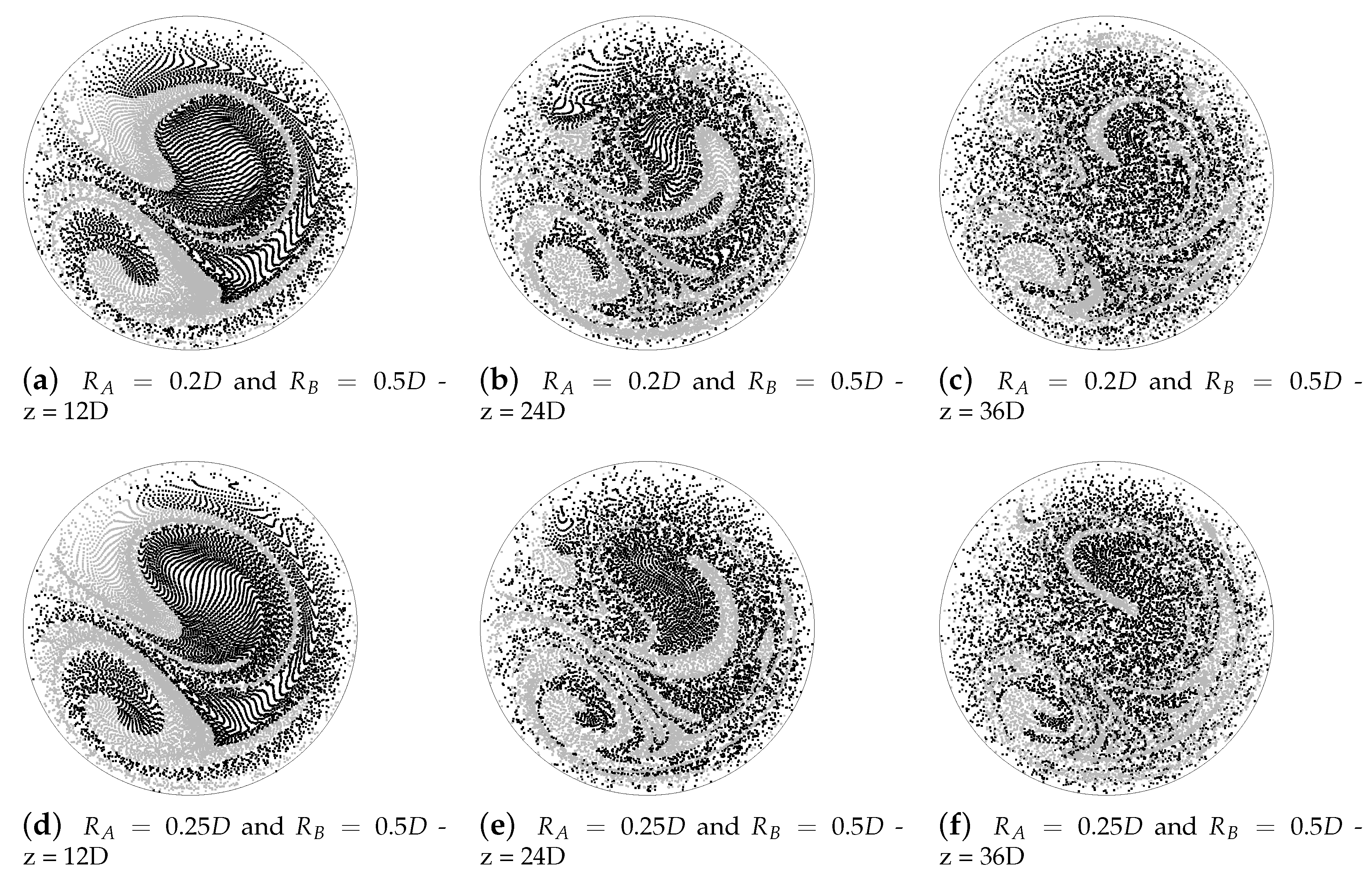
4.1.1. Visual Representation of Mixing Structures

It is instructive to examine the particle trajectory slices for any visible mixing structures that appear at each successive cross-sectional slice. Consider the case of a single helical geometry, $R=0.25D$, shown in Figure 5. Though the particles are becoming increasingly well-mixed, with grey particles initially near the wall brought into the core, the double-vortex structure of the secondary flow is well preserved even after five helical pitch lengths $(z=30D)$. This is a visual indication that the mixing achievable by a single helical pipe is ultimately limited, and that to greatly improve mixing quality requires that this large structure be destroyed.

Figure 6 shows particle trajectory slices at two, four, and six pitch lengths (i.e., $z=12D$, $z=24D$, and $z=36D$ respectively) for four different combined geometries, generated using the idealised prediction. These images demonstrate qualitatively the improvements in mixing that arise when varying the helical radius in an alternating sequence. However, it is clear from Figure 6a–f that when the difference in the velocity fields between the two geometries is not large, such as for [$R_A=0.25D$ and $R_B=0.2D$] and [$R_A=0.35D$ and $R_B=0.3D$], then the underlying vortical structures remain somewhat visible in the particle trajectory plots (though slightly less obvious than for the single helical pipe in Figure 5). When the velocity fields do differ more, for example by angle of vortical dividing line and/or vortical structure asymmetry, as for [$R_A=0.5D$ and $R_B=0.2D$] and [$R_A=0.5D$ and $R_B=0.25D$], the vortical structures that exist in each of the helical pipes used in the combined geometry no longer remain visible in these particle plots, as Figure 6g–l demonstrate.

4.1.2. Entropic Measure of Mixing Performance

Although a total of 11 combined geometries were studied using the idealised prediction, four of these cases will be examined in detail, however the mixing quality will be presented for all cases in Figure 7. These four geometries are: [$R_A=0.25D$ and $R_B=0.2D$], [$R_A=0.35D$ and $R_B=0.3D$], [$R_A=0.5D$ and $R_B=0.2D$] and [$R_A=0.5D$ and $R_B=0.25D$]. Figure 7 shows the relative entropy increase, $\kappa$, evaluated at six pitch lengths of a single geometry $(z=36D)$, which corresponds to three repetitions of a combined geometry. The results are plotted against the normalised pressure drop, which is computed by normalising the axial pressure loss in the helical pipe by the pressure loss that occurs in a straight pipe with Poiseuille flow of the same Reynolds number, over the equivalent axial (point-to-point) distance.

It is assumed at this point that the total pressure drop in the combined geometries can be approximated as the sum of the pressure drops that occur in each of the helical pipes used in the combined geometry. Though it is known that the transition between the two velocity fields will incur an additional pressure drop, it is thought that this will not significantly affect the ranking of the results. The black lines on the plot represent the trend for the single helical geometries and this indicates that all the combined geometries tested, apart from one, achieve better mixing than the single geometries. This geometry is $R_A=0.35D$ and $R_B=0.3D$, which Table 1 shows as having a 6 degree angle between the in-plane vortices. It does however achieve mixing slightly better than that produced by a single helical pipe with either $R=0.35D$ or $R=0.3D$.

4.1.3. Poincaré Sections and Residence Times

The benefit of the combined helical geometries is most directly observed by comparing the single geometry considered to be optimal, $R=0.25D$, and the combination $R_A=0.3D$ and $R_B=0.2D$. These two cases exhibit approximately equal pressure losses, however, the combined geometry generates a $60\%$ improvement in $\kappa$. The reason is clear from the Poincaré section, Figure 8b, which possesses a relatively small island of regular flow, in the lower-left portion of the cross-section, a stark contrast to the two large areas of islands that fill the cross-section for $R=0.25D$ as shown in Figure 5. The geometries possessing the best overall mixing are $R_A=0.5D$ and $R_B=0.2D$, and $R_A=0.5D$ and $R_B=0.25D$, having approximately the same value of $\kappa$, and both showing an improvement of $70\%$ in mixing quality.

Islands of regular flow are a common feature in many of the plots in Figure 9 and reduce the mixing effectiveness of a device. In these cases the islands have formed due to the large degree of overlap of the streamlines for each component geometry in that part of the cross-section, and the greater the overlap, the larger the island. If considered individually, the flows in a single helical geometry would exhibit similar islands. The low residence time value is due to the peak axial velocities also occurring in this region. A similar island forms in the upper-right quadrant of the cross-section when any geometry of $R>0.25D$ is paired with another of $R>0.25D$, again due to overlap of secondary flows in this region. These plots show that pairing one geometry with $R=0.2D$ eliminates the island in the upper-right quadrant, due to the upper-vortex in the $R=0.2D$ velocity field being very different in size, geometry and orientation, from those for $R>0.25D$, thus increasing the degree of streamline transversality.

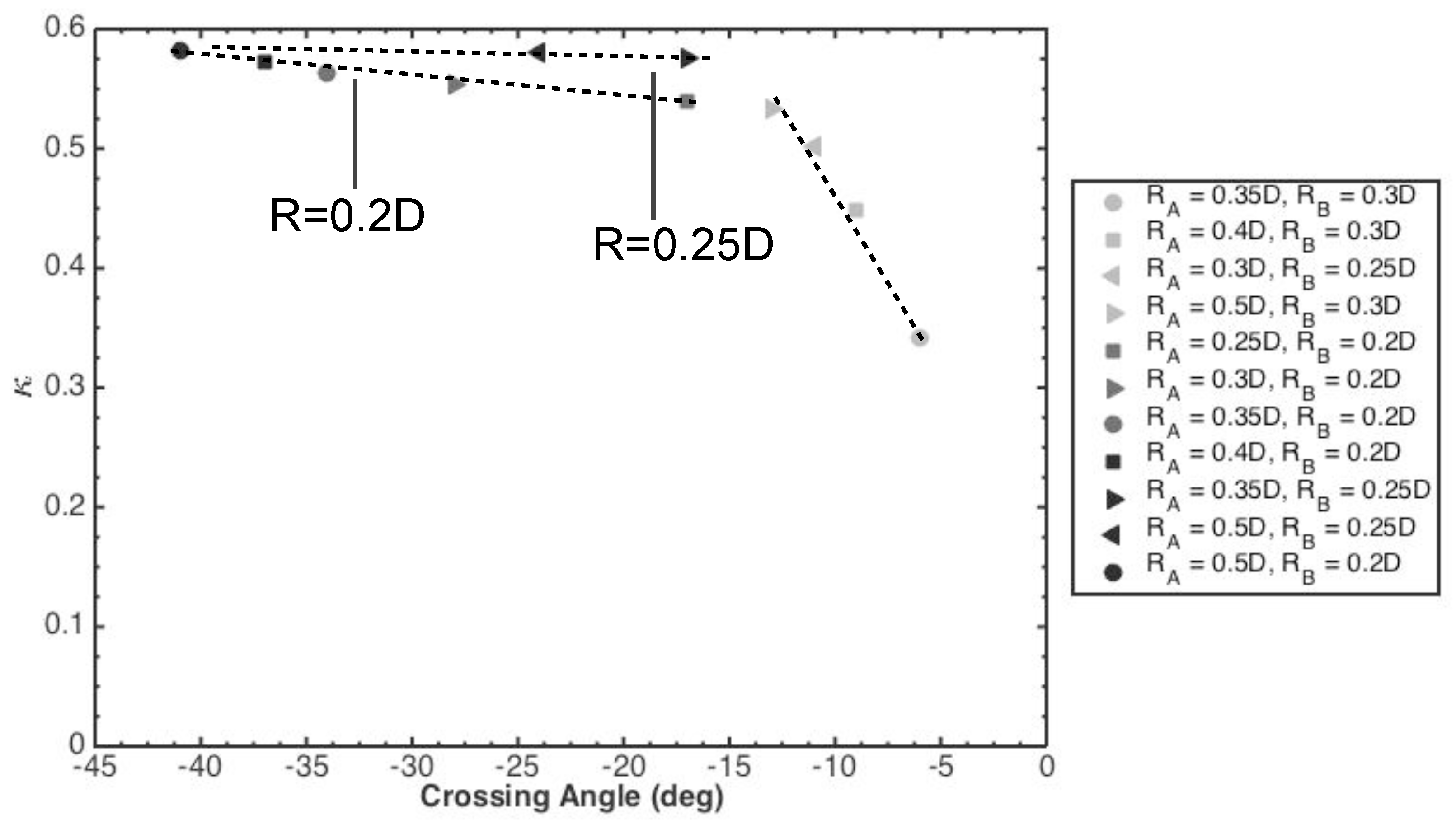
4.1.4. Significance of Crossing Angle

The crossing angle of the vortex dividing lines was the key selection criteria for the geometries, with the results of Jones et al. [28] suggesting that increasing this angle would cause a corresponding increase in mixing. Figure 10 shows the relative entropy increase, $\kappa$, plotted against this angle. In the range 5 to 15 degrees, there is an approximately-linear positive relationship between the two quantities. However, for angles above 17 degrees there appears to be two separate relationships, which are both marked on the plot in Figure 10.

This dual valued relation occurs due to the effect of a confounding variable that the plot does not capture. At an angle of 17 degrees there are two different data points, with the lower point corresponding to a geometry $R_A=0.25D$ and $R_B=0.2D$, and the upper point corresponding to $R_A=0.35D$ and $R_B=0.25D$. The magnitude of ${\mathbf{V}}_{in-plane}$, i.e., the in-plane streamlines, for $R=0.2D$ is smaller than that for both $R=0.25D$ and $R=0.35D$. Therefore, although the overall crossing angle is the same, the particles in the geometry $R_A=0.35D$ will be advected further in each pitch length of the geometry, causing greater stretching of material lines, and generating better mixing of the initial distribution of particles. This weaker in-plane flow is only overcome when coupled with $R=0.5D$, which has the strongest in-plane flow of all the geometries, and also generates the largest crossing angle.

The other factor which prevents a straightforward relation between $\kappa$ and crossing angle, is that the crossing angle is a bulk characteristic that does not account for the change in distribution of vortical structures with R, and therefore, the angle of streamline crossing distributed throughout the cross-section, may be indicative of a greater crossing angle, than that given from the vortex dividing lines. For example, the Poincaré section for $R_A=0.35D$ and $R_B=0.25D$ shows a smaller island of regular flow in the lower-left part of the domain, than exists for $R_A=0.25D$ and $R_B=0.2D$, which can be attributed to greater local streamline crossing angles.

From the results for $\kappa$, the geometries $R_A=0.5D$ and $R_B=0.2D$, and $R_A=0.5D$ and $R_B=0.25D$, generated the most mixing after six pitch lengths. Based on a comparison of the residence time distributions in Figure 9, it is thought that of these two, that with $R_A=0.5D$ and $R_B=0.2D$ may be the slightly more effective mixing device, particularly as axial distance tends to infinity, as the islands in the residence time distribution are smaller than for $R_B=0.25D$. On the other hand, with $R_B=0.25D$, the geometry shows a slightly lower pressure loss, which may make this latter choice more favourable for use as a prosthetic graft.

4.2. Comparison of Predicted and Actual Mixing Behaviour of Combined Helical Geometries

The idealised prediction of mixing has identified two promising geometries, with approximately equal mixing quality. In order to test the validity of the prediction, and discern which of the two geometries is in fact the better mixing device, the ‘true’ mixing performance was calculated using the method described in Section 3.2. Note that although the order of $R_A$ and $R_B$ has been swapped from Section 4.1, this is unimportant due to the periodic nature of the velocity field solutions obtained here.

4.2.1. Entropic Measure

Figure 11 shows the evolution of relative entropy increase, $\kappa$, with axial distance for both geometries, for both the idealised model presented in Section 4.1 and using the velocity field directly computed over the entire combined geometry. From the examination of ${\mathbf{V}}_{in-plane}$ and the particle trajectory slices of Figure 12a–c and Figure 12d–f it is expected that the values of $\kappa$ will be similar for both geometries, but slightly larger for $R_A=0.2D$. Indeed, this is the case, with the presence of the small region of no-mixing likely accounting for the smaller value of $\kappa$ for $R_A=0.25D$.

The predicted and actual values of $\kappa$ are close for both cases, however, the difference is larger for $R_A=0.2D$. This is because the difference between the velocity fields of the component helical geometries is also larger and therefore the velocity field in the combined geometry deviates more from the idealised prediction, than it does for $R_A=0.25D$, where the difference is smaller. Indeed, examining ${\mathbf{V}}_{in-plane}$ for $R_A=0.25D$ and $R_B=0.5D$ in Figure 13 shows a better correspondence to the respective single helical velocity fields, and for more of the geometry, than is the case for $R_A=0.2D$ in Figure 14. For both geometries, the slightly larger value of $\kappa$ compared with the predicted value is possibly due to the larger magnitudes of the velocity ${\mathbf{V}}_{in-plane}$, which will advect the particles a longer distance in each pitch length of the geometry, therefore enhancing the rate of mixing, if not the structure itself.

The close agreement of the predicted value of $\kappa$ to the actual value, means that the idealised model of Section 4.1 is a useful tool for guiding designs. It is computationally cheaper to solve for the velocity field, and track particles through single helical geometries, than it is the combined geometries. Therefore, a larger portion of the parameter space can be investigated using the idealised model, than would be possible using the methodology presented by the authors in [37].

4.2.2. Axial Pressure Loss

Table 3. Normalised pressure losses $\Delta \tilde{p}$, at $Re=250$, calculated by solving the velocity field in the full combined geometry, compared with the predicted loss, calculated by simply summing the normalised pressure losses from the component velocity fields (see Section 4.1).

${\mathit{R}}_{\mathit{A}}$	${\mathit{R}}_{\mathit{B}}$	$\mathbf{\Delta }\tilde{\mathit{p}}$ — Predicted	$\mathbf{\Delta }\tilde{\mathit{p}}$ — Actual	$\mathbf{\Delta }\tilde{\mathit{p}}$ — Increase
0.2D	0.5D	2.08	2.21	5.86%
0.25D	0.5D	2.22	2.26	1.76%

shows the pressure loss for both of the combined geometries examined, at a Reynolds number of 250. The agreement for all cases is good, with no more than $6\%$ deviation. For the case $R_A=0.25D$ and $R_B=0.5D$ the difference is much smaller, less than $2\%$. This is due to the smaller difference between the component velocity fields—as the difference in component fields grows, so will the additional pressure loss. An avenue for future research could be to explore the influence that the Reynolds number has on agreement between the idealised prediction and full computation of the combined geometries, both in terms of pressure loss and mixing quality.

The velocity fields for the combined geometries, shown in Figure 13 and Figure 14, show some variation from the single helix solutions for at least half of the axial distance. However, the velocity fields do approach tend to the single helix solutions at 75–100% of the geometry, i.e., $z=4.5D-6.0D$ and $z=10.5D-12.0D$, as appropriate. However, the pressure drop appears to be well predicted, and with sufficient accuracy for it to be used as a basis for design decisions, particularly with the knowledge that the bigger the difference between component velocity fields, the larger the error will be, in both the pressure loss and $\kappa$. However, these results demonstrate that a strict discontinuity between velocity fields is not necessary for generating the mixing, that even a gradual change between two different flow states is sufficient.

4.3. Poincaré Sections and Residence Times

Figure 15 shows the Poincaré sections and residence time distributions for the full computations for the geometries $R_A=0.25D$ and $R_B=0.5D$ and $R_A=0.2D$ and $R_B=0.5D$. There is a general similarity with these results and those from the idealised simulations in Figure 9f,h though some of the fine structures in the Poincaré sections visible here are missing in those figures. From the residence time distributions it appears that the mixing is slightly more complete in the core of the flow, however both sets of results show an area of very low residence time in the lower-left quadrant, which corresponds to the location of the peak axial velocity. Comparing these results with that for the combination $R_A=0.25D$ and $R_B=0.2D$ in Figure 9a shows the benefits that additional mixing has on reducing the higher levels of residence time in the cross-section. This reduction in residence time, and in extreme values of residence time, is hypothesised to be one of the mechanisms by which the enhanced fluid mixing generated by these combined helical geometries could help to reduce the incidence of thrombosis within the graft.

4.4. Limitations

Several modelling assumptions have been made in this work. The first is of Newtonian blood rheology, which has been found to be a reasonable approximation for flow in the larger blood vessels [53]. The second assumption is of steady flow boundary conditions. For modelling the flow in A-V shunts this is deemed quite realistic, as relatively low levels of pulsatility have been observed in these flows, for example during renal dialysis access [2]. In arterial flow through grafts and stents it is a poorer approximation, however a significant fraction of the physiological pulsatile flow profile is quasi-steady and thus vortical structures during this period may be similar. However, given that flow unsteadiness has been noted to play a role in vascular fluid mixing [54], it is likely that the steady flow assumption used here provides a conservative estimate of the total mixing generated by these combined geometries. In future work, understanding the interaction of flow pulsatility and mixing in combined helical geometries will be an important task.

Related to the assumption of steady flow, is the use of a periodic boundary condition in the axial direction. This is a highly useful construction for understanding the fundamentals of flow in pipes, however in a practical scenario there would be a finite entrance length in the inlet to the helical pipe. The results of the full velocity field computations in the combined geometries suggest that for the Reynolds number under consideration, the flow would develop to the helical pipe solution within a quarter to a half of a pitch length, and therefore this entrance length effect can be neglected in a graft spanning multiple pitch lengths. Finally, the effects of wall compliance have also been neglected, since with a steady flow boundary condition the associated impact would be a slight taper in the z-direction, which would not have any significant effect on the flow.

4.5. Significance for Future Work

As discussed in Section 1, an additional benefit of helical geometries is that they appear to be mechanically resistant to kinking, helping to preserve their fluid mechanical properties after surgical implantation. However, the discontinuous gradient that occurs between two different helical pipes could be a weakness from this point of view. By blending between the two pipes using a spline fit, as was performed for the full simulations, this mechanical weakness is removed. Furthermore, since the results show that the idealised prediction of the mixing, obtained by concatenating velocity field solutions from single helical pipes, has excellent agreement with the actual mixing performance, this strict discontinuity is not actually required to generate the enhanced mixing.

The results demonstrate the proof-of-concept that varying the helical radius of a helical pipe in an alternating fashion can achieve significant increases in the fluid mixing generated by that pipe. Given that helical geometries are already being deployed as grafts and stents, this concept is therefore also appropriate for use in a range of vascular prostheses. The specific choice of the optimal helical radii for these devices would depend on the Reynolds number of the particular application, due to the change in secondary flow structures that occurs with Reynolds number. A selection of simulations performed for both lower [37] and higher Reynolds numbers [1], up to $Re=500$, show that the same phenomena are apparent, with just the precise size and orientations of the vortical structures changing for a given helical geometry. However, the use of the idealised approach would need to be checked if used for substantially larger values of Reynolds number, due to the increase in flow transition distance between helical pipes as Reynolds number increases. Additionally, as described in Section 4.4, examining the role of flow unsteadiness within these devices will be an important task.

Performing one full velocity field computation of a combined geometry takes at least twice as long as performing the two separate single helix simulations. However, the computational saving is even greater when considering the possible combinations of helical geometries. For N parameter value samples, the number of combinations to be tested is the triangular number, $N(N+1)/2$ (given that the order of the two pipes is unimportant). Therefore as N is increased due to a denser sampling of parameter values and the parameter space extended to include varying helical pitch length, the computational effort may be reduced by at least one order of magnitude using the approach proposed in this paper. Further savings in effort would be made if the study included altering the relative lengths of each separate helical geometry. Pursuing such as an approach would likely enable even greater improvements in fluid mixing to be obtained when applying this concept to the design of future vascular devices such as shunts, grafts, and stents.

5. Conclusions

Helical geometries have been previously proposed and tested for use as vascular prostheses such as shunts and stents, due to the swirling flow and in-plane mixing that are induced by the helical geometry, which are thought to reduce thrombosis and neo-intimal hyperplasia. It was hypothesised here that by combining helical pipes of differing helical radius, in series, a large improvement in fluid mixing quality could be achieved compared to single helical geometries. The results show that the idealised method of mixing prediction by concatenating single velocity fields has excellent agreement with full simulations, with both methods showing that a $70\%$ increase in mixing efficiency was generated for the combination $R_A=0.2D$ and $R_B=0.5D$. These findings carry three key items of significance: the first is that the mixing enhancement does not appear to be dependent on a strict discontinuity existing between velocity fields, as might have been expected. This means that the fluid enhancement is practically realisable. The second is that the idealised simulations provide a computationally efficient means of optimising similar design concepts for different operating conditions and applications in future studies. Finally, and most importantly, the results confirm the hypothesis that it is possible to generate enhanced mixing using combined helical geometries, in a configuration that is suitable for use in vascular prosthesis applications. This enhanced mixing could help to improve the patency of these devices by reducing the incidence of thrombosis and neo-intimal hyperplasia.

References

1. Cookson, A.N.; Doorly, D.J.; Sherwin, S.J. Mixing Through Stirring of Steady Flow in Small Amplitude Helical Tubes. Ann. Biomed. Eng. 2009, 37, 710–721. [Google Scholar] [CrossRef] [PubMed] [Green Version]
2. Caro, C.G.; Cheshire, N.J.; Watkins, N. Preliminary comparative study of small amplitude helical and conventional ePTFE arteriovenous shunts in pigs. J. R. Soc. Interface 2005, 2, 261–266. [Google Scholar] [CrossRef] [PubMed] [Green Version]
3. Taggart, D.P. Current status of arterial grafts for coronary artery bypass grafting. Ann. Cardiothorac. Surg. 2013, 2, 427–430. [Google Scholar] [PubMed]
4. Desai, M.; Seifalian, A.M.; Hamilton, G. Role of prosthetic conduits in coronary artery bypass grafting. Eur. J. Cardio-Thorac. Surg. 2011, 40, 394–398. [Google Scholar] [CrossRef] [PubMed]
5. Akoh, J.A. Prosthetic arteriovenous grafts for hemodialysis. J. Vasc. Access 2009, 10, 137–147. [Google Scholar] [CrossRef] [PubMed]
6. Murphy, E.A.; Boyle, F.J. Reducing In-Stent Restenosis Through Novel Stent Flow Field Augmentation. Cardiovasc. Eng. Technol. 2012, 3, 353–373. [Google Scholar] [CrossRef] [Green Version]
7. Garg, S.; Serruys, P.W. Coronary stents: Current status. J. Am. Coll. Cardiol. 2010, 56, S1–S42. [Google Scholar] [CrossRef] [PubMed]
8. Caro, C.G.; Doorly, D.J.; Tarnawski, M.; Scott, K.T.; Long, Q.; Dumoulin, C.L. Non-Planar Curvature and Branching of Arteries and Non-Planar-Type Flow. Proc. Math. Phys. Eng. Sci. 1996, 452, 185–197. [Google Scholar]
9. Huijbregts, H.J.T.A.M.; Blankestijn, P.J.; Caro, C.G.; Cheshire, N.J.W.; Hoedt, M.T.C.; Tutein Nolthenius, R.P.; Moll, F.L. A Helical PTFE Arteriovenous Access Graft to Swirl Flow Across the Distal Anastomosis: Results of a Preliminary Clinical Study. Eur. J. Vasc. Endovasc. Surg. 2007, 33, 472–475. [Google Scholar] [CrossRef] [PubMed] [Green Version]
10. Van Doormaal, M.A.; Ethier, C.R. Design optimization of a helical endothelial cell culture device. Biomech. Model. Mechanobiol. 2010, 9, 523–531. [Google Scholar] [CrossRef] [PubMed]
11. Coppola, G.; Caro, C. Arterial geometry, flow pattern, wall shear and mass transport: Potential physiological significance. J. R. Soc. Interface 2009, 6, 519–528. [Google Scholar] [CrossRef]
12. Coppola, G.; Caro, C. Oxygen mass transfer in a model three-dimensional artery. J. R. Soc. Interface 2008, 5, 1067–1075. [Google Scholar] [CrossRef] [PubMed] [Green Version]
13. Lee, K.E.; Lee, J.S.; Yoo, J.Y. A numerical study on steady flow in helically sinuous vascular prostheses. Med. Eng. Phys. 2011, 33, 38–46. [Google Scholar] [CrossRef] [PubMed]
14. Ha, H.; Hwang, D.; Choi, W.R.; Baek, J.; Lee, S.J. Fluid-Dynamic Optimal Design of Helical Vascular Graft for Stenotic Disturbed Flow. PLoS ONE 2014, 9, e11104. [Google Scholar] [CrossRef] [PubMed]
15. Zheng, T.; Fan, Y.; Xiong, Y.; Jiang, W.; Deng, X. Hemodynamic performance study on small diameter helical grafts. ASAIO J. 2009, 55, 192–199. [Google Scholar] [CrossRef]
16. Zheng, T.; Wang, W.; Jiang, W.; Deng, X.; Fan, Y. Assessing hemodynamic performances of small diameter helical grafts: Transient simulation. J. Mech. Med. Biol. 2012, 12, 1250008. [Google Scholar] [CrossRef]
17. Van Canneyt, K.; Morbiducci, U.; Eloot, S.; De Santis, G.; Segers, P.; Verdonck, P. A computational exploration of helical arterio-venous graft designs. J. Biomech. 2013, 46, 345–353. [Google Scholar] [CrossRef] [PubMed]
18. Stonebridge, P.A.; Vermassen, F.; Dick, J.; Belch, J.J.F.; Houston, G. Spiral Laminar Flow Prosthetic Bypass Graft: Medium-Term Results From a First-In-Man Structured Registry Study. Ann. Vasc. Surg. 2012, 26, 1093–1099. [Google Scholar] [CrossRef]
19. El Sayed, H.F.; Davies, M. Early Results of Using the Spiral Flow AV Graft: Is It a Breakthrough Solution to a Difficult Problem? J. Vasc. Surg. 2015, 62, 811. [Google Scholar] [CrossRef]
20. Ruiz-Soler, A.; Kabinejadian, F.; Slevin, M.A.; Bartolo, P.J.; Keshmiri, A. Optimisation of a Novel Spiral-Inducing Bypass Graft Using Computational Fluid Dynamics. Sci. Rep. 2017, 7, 1865. [Google Scholar] [CrossRef]
21. Kabinejadian, F.; McElroy, M.; Ruiz-Soler, A.; Leo, H.L.; Slevin, M.A.; Badimon, L.; Keshmiri, A. Numerical Assessment of Novel Helical/Spiral Grafts with Improved Hemodynamics for Distal Graft Anastomoses. PLoS ONE 2016, 11, e0165892. [Google Scholar] [CrossRef]
22. Caro, C.G.; Seneviratne, A.; Heraty, K.B.; Monaco, C.; Burke, M.G.; Krams, R.; Chang, C.C.; Gilson, P.; Coppola, G. Intimal hyperplasia following implantation of helical-centreline and straight-centreline stents in common carotid arteries in healthy pigs: Influence of intraluminal flow. J. R. Soc. Interface 2013, 10, 20130578. [Google Scholar] [CrossRef]
23. Shinke, T.; Mullins, L.P.; O’Brien, N.; Heraty, K.B.; McMahon, T.; Burke, M.G.; Taylor, C.; Gilson, P.; Robinson, K.; Caro, C.G. Abstract 6059: Novel helical stent design elicits swirling blood flow pattern and inhibits neointima formation in porcine carotid arteries. Circulation 2008, 118, S1054. [Google Scholar]
24. Zeller, T.; Gaines, P.A.; Ansel, G.M.; Caro, C.G. Helical Centerline Stent Improves Patency: Two-Year Results From the Randomized Mimics Trial. Circ. Cardiovasc. Interv. 2016, 9, e00293. [Google Scholar] [CrossRef] [PubMed]
25. Sullivan, T.M.; Zeller, T.; Nakamura, M.; Caro, C.G.; Lichtenberg, M. Swirling Flow and Wall Shear: Evaluating the BioMimics 3D Helical Centerline Stent for the Femoropopliteal Segment. Int. J. Vasc. Med. 2018, 2018, 9795174. [Google Scholar] [CrossRef] [PubMed]
26. Rajbanshi, P.; Ghatak, A. Flow through triple helical microchannel. Phys. Rev. Fluids 2018, 3, 024201. [Google Scholar] [CrossRef]
27. Ramstack, J.M.; Zuckerman, L.; Mockros, L.F. Shear-induced activation of platelets. J. Biomech. 1979, 12, 113–125. [Google Scholar] [CrossRef]
28. Jones, S.W.; Thomas, O.M.; Aref, H. Chaotic advection by laminar flow in a twisted pipe. J. Fluid Mech. 1989, 209, 335–357. [Google Scholar] [CrossRef]
29. Aref, H. Stirring by chaotic advection. J. Fluid Mech. 1984, 143, 1–21. [Google Scholar] [CrossRef]
30. Sturman, R.; Ottino, J.M.; Wiggins, S. The Mathematical Foundations of Mixing: The Linked Twist Map as a Paradigm in Applications: Micro to Macro, Fluids to Solids; Cambridge University Press: Cambridg, UK, 2006. [Google Scholar]
31. Sturman, R.; Wiggins, S. Eulerian indicators for predicting and optimizing mixing quality. New J. Phys. 2009, 11, 075031. [Google Scholar] [CrossRef] [Green Version]
32. McIlhany, K.L.; Wiggins, S. Eulerian indicators under continuously varying conditions. Phys. Fluids 2012, 24, 073601. [Google Scholar] [CrossRef]
33. Galaktionov, O.; Anderson, P.; Peters, G.; Meijer, H. Analysis and optimization of Kenics static mixers. Int. Polym. Process. 2003, 18, 138–150. [Google Scholar] [CrossRef]
34. Qian, S.; Bau, H.H. A Chaotic Electroosmotic Stirrer. Anal. Chem. 2002, 74, 3616–3625. [Google Scholar] [CrossRef]
35. Moore, J.A.; Steinman, D.A.; Prakash, S.; Johnston, K.W.; Ethier, C.R. A Numerical Study of Blood Flow Patterns in Anatomically Realistic and Simplified End-to-Side Anastomoses. J. Biomech. Eng. 1999, 121, 265–272. [Google Scholar] [CrossRef] [PubMed]
36. Sherwin, S.J.; Shah, O.; Doorly, D.J.; Peiro, J.; Papaharilaou, Y.; Watkins, N.; Caro, C.G.; Dumoulin, C.L. The Influence of Out-of-Plane Geometry on the Flow Within a Distal End-to-Side Anastomsis. ASME J. Biomech. 2000, 122, 86–95. [Google Scholar] [CrossRef]
37. Cookson, A.N.; Doorly, D.J.; Sherwin, S.J. Using coordinate transformation of Navier-Stokes equations to solve flow in multiple helical geometries. J. Comput. Appl. Math. 2009, 234, 2069–2079. [Google Scholar] [CrossRef]
38. Koberg, W.H. Turbulence Control for Drag Reduction with Active Wall Deformation. Ph.D. Thesis, Imperial College London, London, UK, 2008. [Google Scholar]
39. Darekar, R.M.; Sherwin, S.J. Flow Past a Bluff Body With A Wavy Stagnation Face. J. Fluids Struct. 2001, 15, 587–596. [Google Scholar] [CrossRef]
40. Darekar, R.M.; Sherwin, S.J. Flow past a square-section cylinder with a wavy stagnation face. J. Fluid Mech. 2001, 426, 263–295. [Google Scholar] [CrossRef] [Green Version]
41. Newman, D. A Computational Study of Fluid/Structure Interactions: Flow-Induced Vibrations of a Flexible Cable. Ph.D. Thesis, Princeton University, Princeton, NJ, USA, 1996. [Google Scholar]
42. Evangelinos, C. Parallel Spectral/hp Methods and Simulations of Flow/Structure Interactions. Ph.D. Thesis, Brown University, Providence, RI, USA, 1999. [Google Scholar]
43. Sherwin, S.J.; Karniadakis, G.E. Spectral/hp Element Methods for Computational Fluid Dynamics; Oxford Science Publications: Oxford, UK, 2005. [Google Scholar]
44. Doorly, D.J.; Sherwin, S.J.; Franke, P.T.; Peiro, J. Vortical flow structure identification and flow transport in arteries. Comput. Methods Biomech. Biomech. Eng. 2002, 5, 261–275. [Google Scholar] [CrossRef] [PubMed]
45. Coppola, G.; Sherwin, S.J.; Peiro, J. Non-linear particle tracking for high-order elements. J. Comput. Phys. 2001, 172, 356–386. [Google Scholar] [CrossRef]
46. Shannon, C.E. A Mathematical Theory of Communication. Bell Syst. Tech. J. 1948, 27, 379–423. [Google Scholar] [CrossRef]
47. Wang, W.; Manas-Zloczower, I.; Kaufman, M. Entropic characterization of distributive mixing in polymer processing equipment. AIChE J. 2003, 49, 1637–1644. [Google Scholar] [CrossRef]
48. Kang, T.G.; Kwon, T.H. Colored particle tracking method for mixing analysis of chaotic micromixers. J. Micromech. Microeng. 2004, 14, 891. [Google Scholar] [CrossRef]
49. Nielsen, L.B. Transfer of low density lipoprotein into the arterial wall and risk of atherosclerosis. Atherosclerosis 1996, 123, 1–15. [Google Scholar] [CrossRef]
50. Danckwerts, P.V. The Definition and Measurement of Some Characteristic Mixtures. Appl. Sci. Res. 1952, A3, 279. [Google Scholar] [CrossRef]
51. Khakhar, D.V.; Franjione, J.G.; Ottino, J.M. A case study chaotic mixing in deterministic flows: The partitioned pipe mixer. Chem. Eng. Sci. 1987, 42, 2909–2926. [Google Scholar] [CrossRef]
52. Mezic, I.; Wiggins, S.; Betz, D. Residence-time distributions for chaotic flows in pipes. Chaos 1999, 9, 173–182. [Google Scholar] [CrossRef] [PubMed] [Green Version]
53. Friedman, M.H. Arteriosclerosis research using vascular flow models: From 2-D branches to compliant replicas. J. Biomech. Eng. 1993, 115, 595–601. [Google Scholar] [CrossRef]
54. Doorly, D.J. Flow Transport In Arteries. In Cardiovascular Flow Modelling and Measurement with Application to Clinical Medicine; Sajjadi, S.G., Nash, G.B., Rampling, M.W., Eds.; Oxford University Press: Oxford, UK, 1999; pp. 67–81. [Google Scholar]
Figure 1. Demonstration of the concept of streamline crossing, which Jones et al. [28] found to produce excellent mixing through chaotic advection in the twisted pipe configuration in (d). The same streamline crossing can be embodied in helical geometries by combining pipes of differing radius in a series configuration. (Figure 1e–g reprinted from Journal of Computational and Applied Mathematics, Volume 234, Issue 7, A. N. Cookson, D. J. Doorly, S. J. Sherwin, Using coordinate transformation of Navier—Stokes equations to solve flow in multiple helical geometries, pp. 2069–2079, Copyright (2009), with permission from Elsevier.)
Fluids 04 00059 g001
Figure 2. The helical geometries studied here have a small amplitude, R, relative to the pitch length. In (c,e,g) the green circle indicates the pipe boundary and the larger black circle indicates the bounding cylinder of the pipe. The dashed circle represents the axial line-of-sight that can exist for small amplitude helical pipes—note that this line-of-sight just disappears when R = 0.5 D , as seen in (g).
Fluids 04 00059 g002
Figure 3. In-plane streamtraces and contours of in-plane velocity magnitude for a single helical geometry—for R = 0.2 D a second vortical structure emerges in the upper-right portion of the cross-section. As R is increased, this second vortex increases in size and the dividing line between the two vortices tends towards the horizontal. (Reprinted from Journal of Computational and Applied Mathematics, Volume 234, Issue 7, A. N. Cookson, D. J. Doorly, S. J. Sherwin, Using coordinate transformation of Navier—Stokes equations to solve flow in multiple helical geometries, pp. 2069–2079, Copyright (2009), with permission from Elsevier.)
Fluids 04 00059 g003
Figure 4. A Poincaré section is formed by taking intersections of a system’s solution trajectories after each iteration/period of the flow. Here a periodic orbit sees a solution return to the same point after each iteration. By contrast, another trajectory, initially starting close to this periodic point moves throughout the domain.
Fluids 04 00059 g004
Figure 5. Coloured particle distributions taken at inlet and after one, three, and five pitch lengths of a single helix for R = 0.25 D —though the particles are gradually mixed with each iteration, the double vortex structure of the secondary flow remains visible even after five pitch lengths. The relevant value of κ is shown below each particle trajectory slice. (Reprinted by permission from: Springer, Annals of Biomedical Engineering, DOI: 10.1007/s10439-009-9636-y, Mixing through stirring of steady flow in small amplitude helical tubes, A. N. Cookson, D. J. Doorly, S. J. Sherwin, (© 2009).)
Fluids 04 00059 g005
Figure 6. Slices of particle trajectories taken at z = 12 D (left), z = 24 D (middle), and z = 36 D (right) for the four combined helical geometries. For cases with only a small change in velocity fields the flow structures are still visible in the particle trajectory slices. However when this change is larger, (gi) and (jl), these structures are much less persistent at z = 36 D .
Fluids 04 00059 g006
Figure 7. Relative entropy increase, κ , plotted against pressure drop, which has been normalised by the Poiseuille pressure drop that would occur over the equivalent axial, point-to-point distance. The black dotted line indicates the mixing trend obtained for the single helical geometries in previous work [1], highlighting the high cost of pressure drop required to achieve limited improvements in mixing in these geometries. These results show that all but one of the combined geometries show a substantial increase in κ for equivalent pressure losses over all the single geometries.
Fluids 04 00059 g007
Figure 8. Initial particle distribution, coloured by total residence time of the particle over six pitch lengths (left) and Poincaré sections generated by 50 iterations of the combined mapping (right). Islands of ’no mixing’ can be seen to correspond in both Poincaré sections and residence times.
Fluids 04 00059 g008
Figure 9. Initial particle distribution, coloured by total residence time of the particle over six pitch lengths (left) and Poincaré sections generated by 50 iterations of the combined mapping (right). Islands of ’no mixing’ can be seen to correspond in both Poincaré sections and residence times.
Fluids 04 00059 g009aFluids 04 00059 g009b
Figure 10. Relative entropy increase, κ , plotted against the crossing angle χ between the vortical dividing lines in the secondary flows of the combined geometries (see Figure 1). If both helical pipes in the combined geometry possess R 0.25 D , the mixing quality shows a monotonic trend. However, if one of the pipes has R = 0.2 D then a non-monotonic dependence of κ on the crossing angle χ is introduced. This is due to the strong asymmetry of the secondary flow structures for the single helical pipe R = 0.2 D , as shown in Figure 3b, which is much less pronounced when R = 0.25 D , as seen in Figure 3c. The existence of this non-monotonic behaviour means that crossing angle χ can not be used as an absolute proxy for mixing quality in contexts where vortical structure asymmetry can also vary significantly between geometries, though these results suggest that any error would be small.
Fluids 04 00059 g010
Figure 11. Relative entropy increase, κ , for combined geometries, showing evolution with axial location, and comparing idealised prediction with particle tracking in the actual velocity field. In both cases the error is small and the trend is predicted correctly. This prediction is more accurate for R A = 0.25 D and R B = 0.5 D , due to the fact that the change in the velocity fields is not as large as for R A = 0.2 D and R B = 0.5 D .
Fluids 04 00059 g011
Figure 12. Particle trajectory slices obtained from particle tracking performed on the velocity field directly computed over the entire combined geometries.
Fluids 04 00059 g012
Figure 13. Streamtraces of V i n p l a n e (cm/s) for R A = 0.25 D and R B = 0.5 D , R e = 250 . (a,b) show the streamtraces from the single helical geometries, with (df) showing results from the combined geometry. The velocity field at z = 0 , in (d), in the combined geometry corresponds closely to that for R = 0.5 D , in (b), whereas at z = 6 D , in (h), the streamtraces are close to those for R = 0.25 D in (a). Note that in contrast to Figure 14, the streamtraces correspond even more closely to those in the single helical geometries, due to the reduced spatial asymmetry in the flow structures between the two component geometries.
Fluids 04 00059 g013
Figure 14. Streamtraces of V i n p l a n e (cm/s) for R A = 0.2 D and R B = 0.5 D , R e = 250 . (a,b) show the streamtraces from the single helical geometries, with (dl) showing results from the combined geometry. The velocity field at z = 0 , in (d), in the combined geometry corresponds closely to that for R = 0.5 D , in (b), whereas at z = 6 D , in (h), the streamtraces are close to those for R = 0.2 D in (a).
Fluids 04 00059 g014
Figure 15. Residence time colour scatter plot (left) and Poincaré sections (right) obtained from particle tracking performed on the velocity field directly computed over the entire combined geometries. A correspondence in structures between the two plots can be observed for R A = 0.25 D and R B = 0.5 D in (a,b).
Fluids 04 00059 g015