Longevity of Enhanced Geothermal Systems with Brine Circulation in Hydraulically Fractured Hydrocarbon Wells

Abstract

A simple, semi-analytical heat extraction model is presented for hydraulically fractured dry reservoirs containing two subparallel horizontal wells, connected by a horizontal fracture channel, using injected brine as the working fluid. Heat equations are used to quantify the heat conduction between fracture walls and circulating brine. The brine temperature profiles are calculated for different combinations of fracture widths, working fluid circulation rates, and initial fracture wall temperatures. The longevity of the geothermal heat extraction process is assessed for a range of working fluid injection rates. Importantly, dry geothermal reservoirs will not recharge heat by the geothermal flux on the time scale of any commercial heat extraction project. A production plan is proposed, with periodic brine circulation maintained in a diurnal schedule with 8 h active production alternating with 16 h of pump switched off. A quasi-steady state is achieved after both the brine temperature and rock temperature converge to a limit state allowing fracture-wall reheating by conduction from the rock interior in the diurnal production schedule. The results of this study could serve as a fast tool for assisting the planning phase of geothermal reservoir design as well as for operational monitoring and management.

1. Introduction

Because of the magmatic intrusions, generation of faults, geothermal fluid convection, and slow decay of radioactive particles in the earth’s interior, the subsurface rock receives continuous heat flow [1], which is known as the geothermal energy. Geothermal fluids and gases surface as hot springs and in volcanic emissions, especially near the edges of the earth’s tectonic plates. Although geothermal energy is abundant throughout the earth, the complexity of the subsurface conditions brings vast challenges for its economic extraction. As of 2015, the US has 3.7 GW installed geothermal power capacity, a major fraction of the world’s 13.3 GW total, making it by far the world’s leading geothermal energy producer [2]. However, as of 2013, geothermal electricity comprises only 0.4% of the total electricity generation in the USA [3].

The current US geothermal power generation capacity (Figure 1a, dotted line) is confined to just six western states (CA, NV, UT, OR, ID, WY). These states have crustal sections with relatively high heat flow locally (SMU Geothermal Map US 2004) [4], which, in combination with local hydrothermal reservoirs, provides favorable conditions for effective heat extraction. The United States Geological Survey (USGS) geothermal resources assessment methodology only considers relatively shallow high temperature (HT) reservoirs, hotter than 150 °C, in crustal regions with high heat flow [5]. Eastern US states generally have lower geothermal gradients, which means high-temperature (HT) geothermal reservoirs can only occur at depths greater than in the western US. For example, West Virginia has HT locations with over 150 °C rocks at 4.5 to 5 km depth [6]. Such low temperature geothermal resources could be used for district heating in colder states [7], whose resource potential is currently not included in the USGS geothermal resource estimation.

Although commercially successful extraction of geothermal energy is only proven profitable for hydrothermal systems, enhanced geothermal systems (EGS) are continuously studied and new design solutions must be developed to render such projects economically viable. When native working fluid is lacking or scant, EGS projects aim to inject enough working fluid and enhance the contact area with the host rock through hydraulic fracturing and hydroshearing of hot dry rock (Figure 1b). Heat is extracted from the circulating working fluid, but EGS reservoirs typically carry heat to the surface much less effectively than hydrothermal systems, making commercial power generation more difficult in EGS projects. Alternatively, heat can be extracted at shallower depths, commonly for water heating, drying processes, and space heating in colder regions, from the ambient rock through heat exchangers (Figure 1b, [10]).

We address, specifically, the need to develop viable solutions for refurbishing depleted shale oil and gas wells, which are already hydraulically fractured for redeployment in EGS projects to extract additional energy (geothermal heat) from the subsurface. A feasibility study is being undertaken to develop a space-conditioning system powered by direct-use of geothermal energy from depleted oil wells at the Texas A&M RELLIS Campus [11]. The semi-analytical model presented in our study aims to provide an initial assessment of the circulation mode required to establish a sustainable geothermal energy extraction rate for such wells.

The extraction of geothermal energy from geothermal target zones using EGS involves increasing the access to the heat source by hydraulic fracture treatment. Additionally, non-hydrothermally wetted rock outside hydrothermal zones are typically dry, and thus a working fluid is lacking and needs to be supplied, for example, by the injection of brine as the working fluid [12]. The Hot Dry Rock (HDR) reservoir is an EGS solution first proposed in 1974 [13], where hydroshearing is applied to interconnect two or more boreholes that penetrate a previously dry geothermal reservoir, to establish within the reservoir a sufficiently large heat-transfer surface so that heat energy can be extracted from the reservoir at a commercial high rate using fluid injection in one borehole and exchange the energy via production well. Brown [14] reviewed 20 years of geothermal energy extraction research by the Los Alamos National Laboratory for the Fenton Hill HDR reservoir. The study summarizes the techniques suggested to efficiently extract the geothermal energy, including heat transfer in the rock mass and associated flow in the rock fractures.

There have been many quantitative studies of the heat flow balance in geothermal energy extraction systems. In this study, we design and numerically simulate a scheme to reuse abandoned horizontal hydrocarbon wells as a geothermal energy source, by circulating brine to pick up heat from the reservoir for use at the surface. Depletion of hydraulically fractured US oil and gas wells in shales may eventually lead to a large number of abandoned wells. These abandoned wells commonly have depths up to several kilometers, where stored geothermal energy is abundant. Repurposing abandoned wells for EGS applications requires the building of a geothermal reservoir model to simulate the fluid flow and temperature distribution of the fluid involved in the production process. A comprehensive geothermal reservoir model needs lots of field data and long computation time. Our study is aimed at improving the analytical model for heat extraction by a working fluid from a fracture system connecting abandoned horizontal wells. We parameterize the problem by assuming that a single horizontal fracture plane connects a horizontal well pair to act as a channel for the injection brine. Heat transfer equations are applied to model the energy transfer mechanisms occurring when brine is injected into underground fracture planes to extract geothermal energy via producer wells. Metrics are provided for collaborating the longevity of the geothermal reservoir in a simplified, but scalable EGS design, for a range of circulation rates.

One of the important findings of our study (Section 3) is that the natural heat flow is not capable of re-heating, on the scale of decades, dry geothermal reservoir rocks cooled by a circulating brine (actually, cold brine in, hot brine out). Unlike hydrothermal systems, where new hot fluid is continually convecting upward from a deeper magmatic heat source to rejuvenate the geothermal reservoir (such as occurs at Neal Hot Springs, Oregon [15]), dry EGS reservoirs lack such rejuvenation. Once cooled, restoration of the geothermal gradient in the EGS volume through conductive heat transfer in dry rock by the local heat flow from the core outward would take thousands of years (Section 3). A similar conclusion was reached by Fox et al. [16], who also stated that a commercial temperature could be maintained.

A recent study of the Neal Hot Springs (NHS) Geothermal Power Plant [15] located at Vale (Oregon, United States) provided a clear benchmark for the volume of working fluid and temperature required to produce electrical energy using existing power generation technology. Given the occurrence of native geothermal brine of 140 °C (285 °F) at about 750 m (~2500 ft) depth, the 22 MW net capacity NHS power plant operates on geothermal energy from just four production wells. The three most productive wells deliver about 3000 gpm each, which corresponds to about 100,000 bbls/day per well (or 184 L/s). For comparison, the high-profile EGS project installed at Rittershoffen, France, has only one production well, which is targeted to extract geothermal fluid of 170 °C (338 °F) at a rate of about 70 L/s [17]. The Rittershoffen EGS project resulted from several decades of research work at nearby Soultz-sous-Forêts, but a suitable fault plane with enhanced hydraulic conductivity was found at Rittershoffen, which is accessed by one injection well and one production well placed about 1 km apart [18]. Above projects indicate that the viability of a geothermal EGS project critically hinges on three basic aspects: (1) Achieving circulation rates of a working fluid with well production rates in the range of 70 L/s (Rittershoffen) to 184 L/s (Neal Hot Springs), (2) extracting such fluid volumes with an appropriate temperature, in the range of 100 to 150 °C, and (3) maintaining both the flux and the temperature over a 20–30 year life-cycle required for any commercial heat conversion project.

This paper is organized as follows. First, we review some of the prior work on EGS and HDR reservoir modeling, with their assumptions, conclusions, and limitations explained, before the novelties of our present study are stated. Second, the possibility of recharging a dry geothermal reservoir by natural geothermal heat flux is investigated and shown to be negligible in terms of the life cycle of a geothermal project. Third, we developed a mathematical model, considering four inter-linked heat transfer mechanisms: (1) Heat transfer from rock to the injected brine; (2) cooling of the rock by the circulation brine; (3) integrated heat transfer between brine and fracture wall; and (4) the heat recovery of the cooled rock by internal thermal diffusion. Fourth, the implications and limitations of various mechanisms are discussed, and an integrated model is simulated to find the optimal circulation plan. Finally, conclusions are drawn, including some hints for practical application.

2. Prior Work and Model Design

2.1. Generic Models and Case Studies

Numerous researchers have contributed to the technical description of HDR reservoirs, proposing heat transfer models for geothermal projects [19,20]. Extensive literature review and work on HDR reservoirs has been summarized in several studies [21,22]. For heat transfer models and their applications in practice, see References [14,23] on classical heat equations and [24,25,26] on fractional heat equations. Several tools have been developed to model the fluid flow and temperature evolution in EGS systems. Geothermal simulation software (such as COMSOL, MultiPhysics (Version 5.3, COMSOL Inc., Stockholm, Sweden), and TOUGH2 (Version 2.0, Berkeley, CA, USA) [27,28,29,30] commonly applies the convection–diffusion equation to model the fluid flow rate in geothermal reservoir. Below, we review the most fundamental studies pertinent to our current approach.

2.2. Analytical Models

Gringarten et al. [31] assumed the fluid flow in a linear model involving an infinite series of parallel, equal-distance, vertical fractures of uniform thickness, separated by blocks of homogeneous and isotropic impermeable rock. The width of the individual fracture was assumed to be negligible in comparison to the spacing between the fractures. Assuming spatial periodicity and similarity of the temperature field, the multiple fracture system is replaced by a single vertical fracture separating two matrix blocks with an insulating outer boundary at a distance from the mid-plane of the fracture equal to half of the fracture spacing. Water is injected at the bottom of the fracture plane and flows upward in the fracture. Other assumptions include: (1) Product of the density and heat capacity for both water and rock is constant; (2) flow rate of the water is constant in the fracture; (3) temperature is uniformly distributed inside the fracture cross-section; (4) heat transfer by radiation within the fracture is negligible; (5) no conduction in the vertical direction of the fracture, and initially, both the water in the fracture and formation are at the same temperature; and (6) there is no external heat flux for heating the system. The authors showed that a multifracture geothermal system could greatly increase the economic utilization of hot dry rock as compared to a single fracture.

Heuer et al. [19] assumed there is only one single fracture in the form of an oval horizontal cylinder. The cold water is incompressible and is injected in one location of the fracture plane. After running across a certain distance in the fracture, the water is extracted at another location on the fracture plane. The fracture is assumed to be a horizontal cylinder with limited height, so that the gravitation effect can be neglected. External heat flux is neglected. The flow is considered to be 2-D so that there is a dipole-flow from the point of injection to the point of extraction. Heat convection is assumed to be dominating over heat conduction within the fracture. Laplace transforms and inverse Laplace transforms were used to derive the temperature distribution on the fracture plane. That study also included a sensitivity study of flow velocity and running distances, which could be used to optimize EGS designs.

Cheng et al. [20] studied the heat extraction by circulating water in a vertical fracture embedded in a geothermal reservoir. The heat conduction in the reservoir is typically assumed to be one dimensional and perpendicular to the fracture. The vertical fracture is assumed to fully penetrate the entire height of the reservoir. The injection well and the extraction well are both vertical. The authors showed that the heat storage and heat dispersion effect are negligible due to dominant advective transport in the fracture channel. A two-dimensional heat conduction model can significantly alter the heat extract temperature and reservoir life as compared to the one-dimensional model.

Martinez et al. [32] proposed an analytical model of heat conduction in fractured rocks. The flow is assumed to be steady state, single phase, incompressible, and laminar. Gravity effects and density variations with temperature are neglected. The infinite fracture walls are smooth and parallel to each other. The rock is assumed to be impervious to the flow. The heat spreads throughout the matrix by conduction. The equations are derived by considering both the longitudinal and transverse dispersion of thermal energy in fractures and rocks. The temperature profile in fracture is derived by assuming complete transverse mixing and negligible longitudinal dispersion. However, the inverse Fourier–Laplace transform is complicated to compute and time consuming. The temperature profile was computed for a 10 m distance along the fracture, which is relatively short and limited for practical applications.

In summary, previous studies included the following basic assumptions. Gringarten et al. [31] assumed the vertical fractures to be infinite so that the inverse Laplace transform could be performed analytically. Heuer et al. [19] assumed the flow patterns to be dipole-flow to simplify the equations so that these could be solved by a Laplace transform and inverse Laplace transform. Cheng et al. [20] assumed the fracture plane to be vertical and infinite. Martinez et al. [32] assumed the fractures and matrix all have infinite length so that the Fourier–Laplace transform could be solved analytically.

Fox et al. [33] reviewed discrete fracture models, proposed a simple analytical model based on Laplace transforms, and compared the results to TOUGH2 solutions with close convergence. Hawkins et al. [34] argued that it is the effective heat transfer area, not the fracture aperture, that dominates heat transport. However, this is too simplistic as exposed fracture surface is only but one aspect. Our present model conclusively demonstrates that fracture aperture influences the heat transfer process.

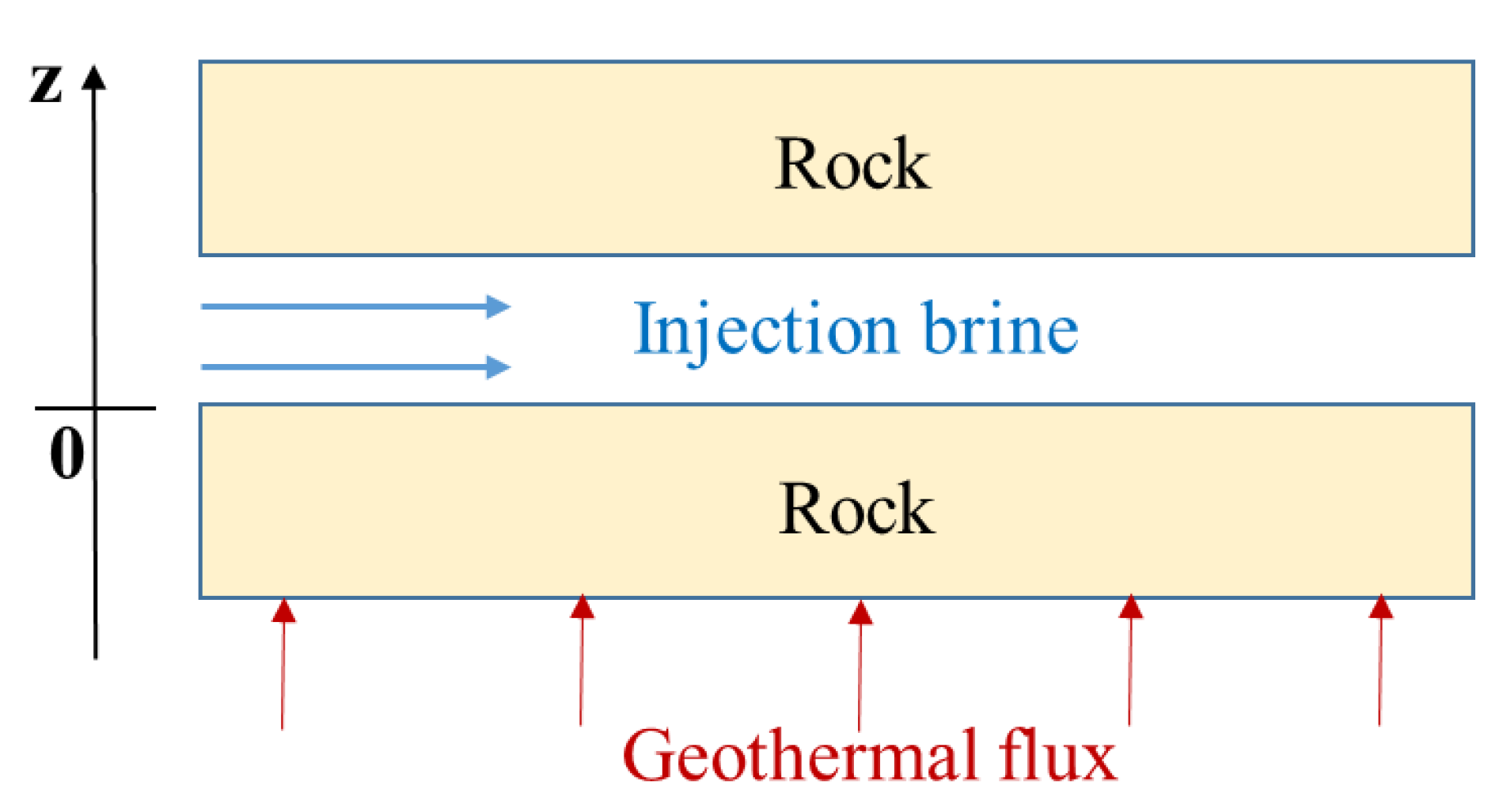
2.3. Model Design Used in This Study

In hydrothermal systems, obviously recharging occurs by hydrothermal circulation of fluid from a magmatic heat source which maintains convective fluid circulation between the deeper heat source and the shallow extraction zone tapped by a spring or a manmade well. Such natural re-charge by native fluids cannot be expected to occur in a dry rock EGS project. In order to quantify the heat delivery capacity and longevity of an EGS reservoir, we consider four principal heat transfer mechanisms between the circulating brine and the rock, each of which cause, partly simultaneous, changes of state:

• Mechanism 1: Heating of the cold injection brine when passing along a hotter fracture wall;
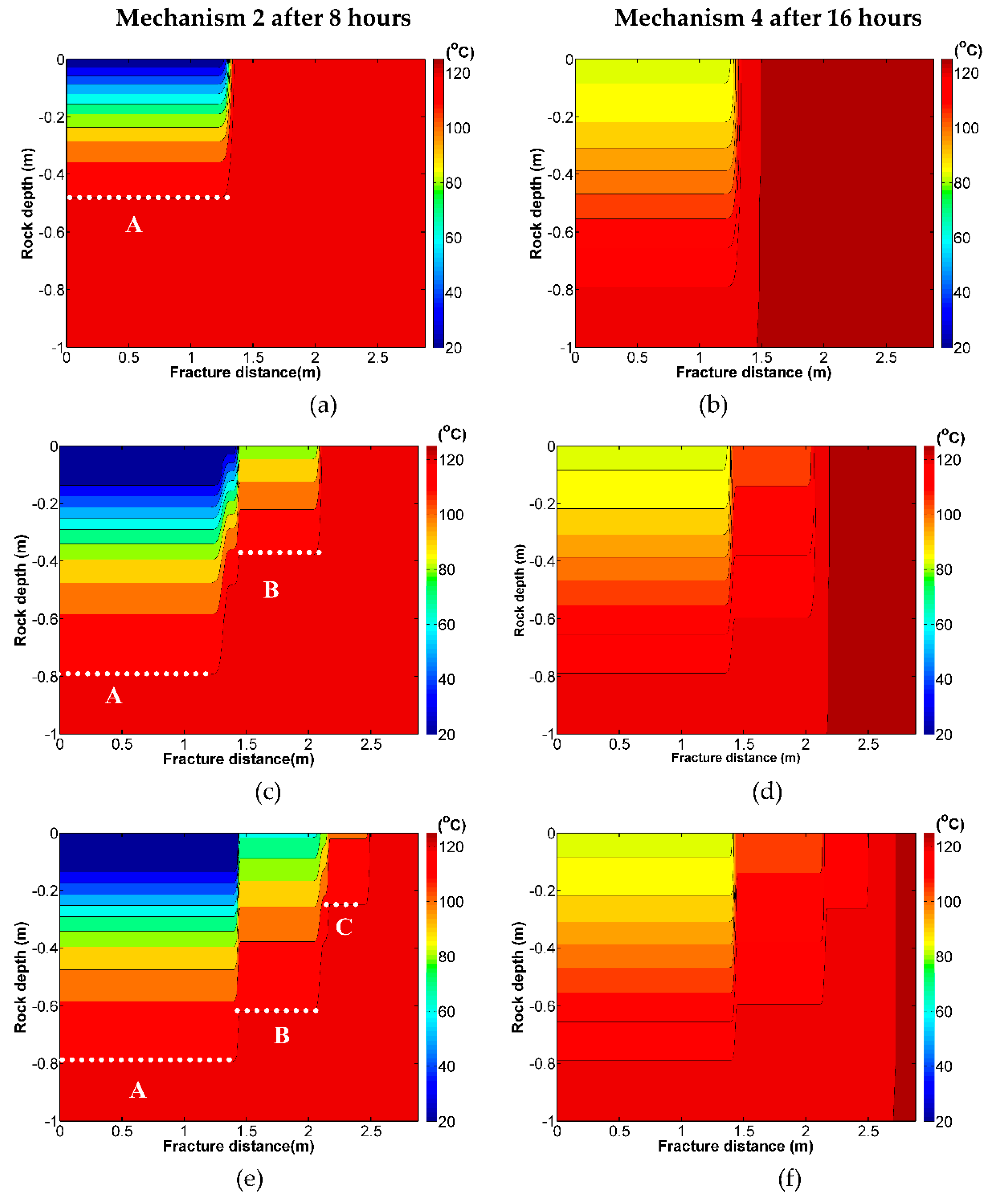
• Mechanism 2: Cooling of the hot rock due to the passing of a colder brine;
• Mechanism 3: The integrated effects of brine-heating and fracture-wall cooling;
• Mechanism 4: Recovery of the cooled fracture wall by “self-heating” via the adjacent deeper, still hot rock, once the injection of the cold brine is (temporarily) halted.

Before examining these four heat transfer mechanisms in detail (Section 3), the overall assumptions of this study are outlined first. Figure 2 shows two horizontal wells of variable mutual distance connected by at least one horizontal fracture, which could be scaled up in case more such fractures exist. The model assumes there exists at least one fracture channel, with a certain length $L$, distance $D$, and aperture $A$. Cold water is injected from the injection well with constant flow rate $Q$. An initial temperature $T_s$, for the fracture wall is assumed to be uniform, which will change when the cold fluid (with initial fixed temperature $T_{mi}$) is injected. The fracture aperture is usually very small (between 0.005 m to 0.01 m). In our model, the temperature $T$ of the injected brine will be calculated for each location $x$ in the direction of flow toward the producer well. This design is considered for implementation in a space-conditioning system powered by geothermal energy from depleted oil wells at the Texas A&M RELLIS Campus [11].

In our study, the fracture length and width are all finite. The interaction of fracture and matrix is studied by discretizing the fracture length to subintervals. The essential features of our study include:

• The fracture plane is horizontal with variable finite length and width; channel flow is assumed within the fracture.
• Flow distance needed to reach a certain temperature is calculated analytically (Equation (7)) for fixed fracture wall temperature.
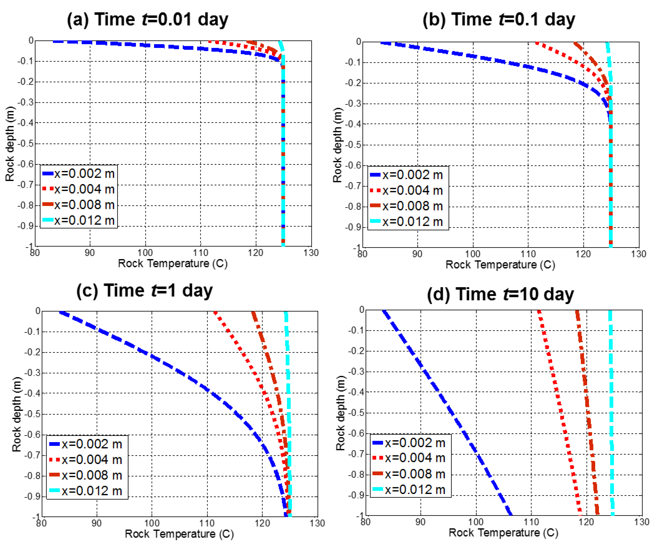
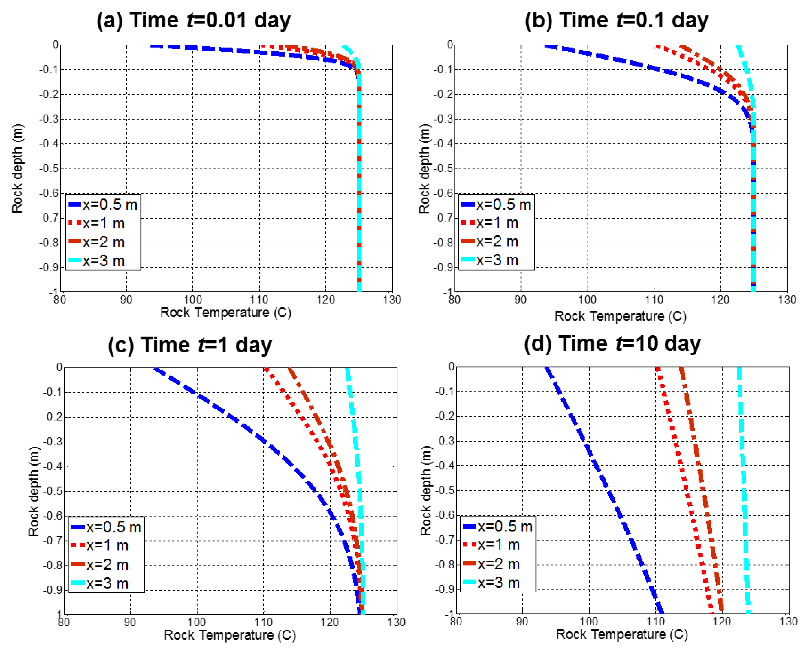
• Thermal conduction in the rock interior adjacent to the fracture wall cooled by the circulating brine is analytically solved (Equation (12)), which gives the rock temperature profile versus rock depth.
• Rock temperature recovery after the fluid circulation stops is calculated explicitly using Fourier transform (Equation (15)).
• Heat transfer between the cooler brine and the hotter wall rock of the fracture is integrated using a semi-analytical method.

2.4. Heat Flow Recharge of EGS Reservoirs

Before modeling the heat transfer between the fluid circulating in a narrow fracture space (Section 3), we investigated the time needed to heat up the rock in an EGS reservoir by the natural geothermal heat flux. Below analysis conclusively shows that the time needed for the natural geothermal heat flux to recharge the EGS reservoir is too long to be considered significant on the time scale of the economic life cycle of any geothermal project.

There are two different methods to formulate heat transfer processes—one assumes the application of heat by assuring a constant surface temperature and the other assumes the existence of a constant heat flux. In this section, we apply a heat transfer model with the assumption that the reservoir rock is heated by a deep-seated, constant heat flux. The deep-seated geothermal heat flux from below ($z=-H$) heats the fractured EGS reservoir rock and the vertical scale is in the z-direction (Figure 3).

Assuming the initial rock temperature is constant, $T_0$, and constant flux on the internal boundary, then the temperature profile of the rock along depth $z$ satisfies the following equation [1],

$$\{\begin{array}{c}\frac{\partial T}{\partial t}=\kappa \frac{{\partial }^{2}T}{\partial z^2},0<z<H\\ T=T_0,z=0\\ \frac{\partial T}{\partial z}=q_f,z=H\end{array}$$

(1)

The solution can be solved as below,

$$T(z,t)=T_0+\frac{2q_f}{k}\left\{\sqrt{\frac{\kappa t}{\pi }}{e}^{\raisebox{1ex}{$-{(H-z)}^2$}\!\left/ \!\raisebox{-1ex}{$4\kappa t$}\right.}-\frac{H-z}{2}\mathrm{erfc}(\frac{H-z}{2\sqrt{\kappa t}})\right\},\left(\mathrm{K}\right)$$

(2)

with geothermal heat flux, $q_f$ ($\mathrm{W}/{\mathrm{m}}^2$), thermal diffusivity $\kappa$, $\kappa =\frac{k}{\rho c}$ (m²/s), and thermal conductivity $k$ (W/m⋅K). On the right-hand side, the unit of $\frac{q_f}{k}$ is $(\frac{\mathrm{W}/{\mathrm{m}}^2}{\mathrm{W}/(\mathrm{m}\cdot \mathrm{K})})=(\frac{\mathrm{K}}{\mathrm{m}})$, and the unit of $\kappa =\frac{k}{\rho c}$ is $(\frac{\mathrm{W}/(\mathrm{m}\cdot \mathrm{K})}{\mathrm{k}\mathrm{g}/{\mathrm{m}}^3\cdot \mathrm{J}/(\mathrm{k}\mathrm{g}\cdot \mathrm{K})})=({\mathrm{m}}^2/\mathrm{s})$, so that $\sqrt{\kappa t}$ has unit m, which means the unit of the expressions inside the “{}” sign of Equation (2) is (m). Thus, the unit for the second term on the right-hand side is K, which matches with the unit of temperature on the left-hand side of Equation (2).

At a certain time, t, the temperature, T, at the fracture surface located at depth z = 0, is specified using a simplified version of Equation (2):

$$T(H,t)=T_0+\frac{2q_f}{k}\left\{\sqrt{\frac{\kappa t}{\pi }}{e}^{\raisebox{1ex}{$-H^2$}\!\left/ \!\raisebox{-1ex}{$4\kappa t$}\right.}-\frac{H}{2}\mathrm{erfc}(\frac{H}{2\sqrt{\kappa t}})\right\} \left(\mathrm{K}\right)$$

(3)

Equation (3) is used to calculate the temperature at the fracture surface, which is in close contact with the injected brine. Assume the initial temperature of the fracture surface and its rock interior have been uniformly cooled to 20 °C, and there is no longer any active cooling mechanism, and re-heating may only occur from below by the geothermal heat flux of 0.06 W/m² [35]. The fracture surface temperature evolution profile is plotted in Figure 4a. The fracture temperature recharge rate is about 1 °C per 300 year.

Figure 4a illustrates that the rock surface temperature will increase very slowly due to the applied geothermal heat flux of 0.06 W/m². In fact, the fracture surface temperature takes about 1500 years to increase another 5 °C. After 2000 years, the fracture surface temperature will only increase to about 26 °C. Any time scale longer than decades is not compatible with the economically useful life cycle of geothermal reservoirs (usually about 25 years).

The temperature increase of the rock interior due to the geothermal heating after five years is plotted in Figure 4b. After t = 5 years, the maximum temperature change is only about 0.5 °C at the geothermal flux location, while the temperature at the fracture surface (depth $z=0$ m) still remains unchanged. The natural geothermal heat flux is initially monitored at a depth $z=-100$ m. Temperatures of a reservoir cooled to 20 °C at −100 m will slowly increase, and only later the rock temperatures at shallower depth may gradually increase, provided cooling from above is neglected.

The temperature increase of any dry geothermal reservoir due to the natural geothermal flux is so slow that it can be neglected over the geothermal project life cycle in our model construction below. If there is no extra heat source, the temperatures of the fracture wall and the interior of the rock will keep decreasing due to colder brine circulation, until the reservoir arrives at the same temperature as the cold brine.

3. Assessment of Heat Transfer Mechanisms

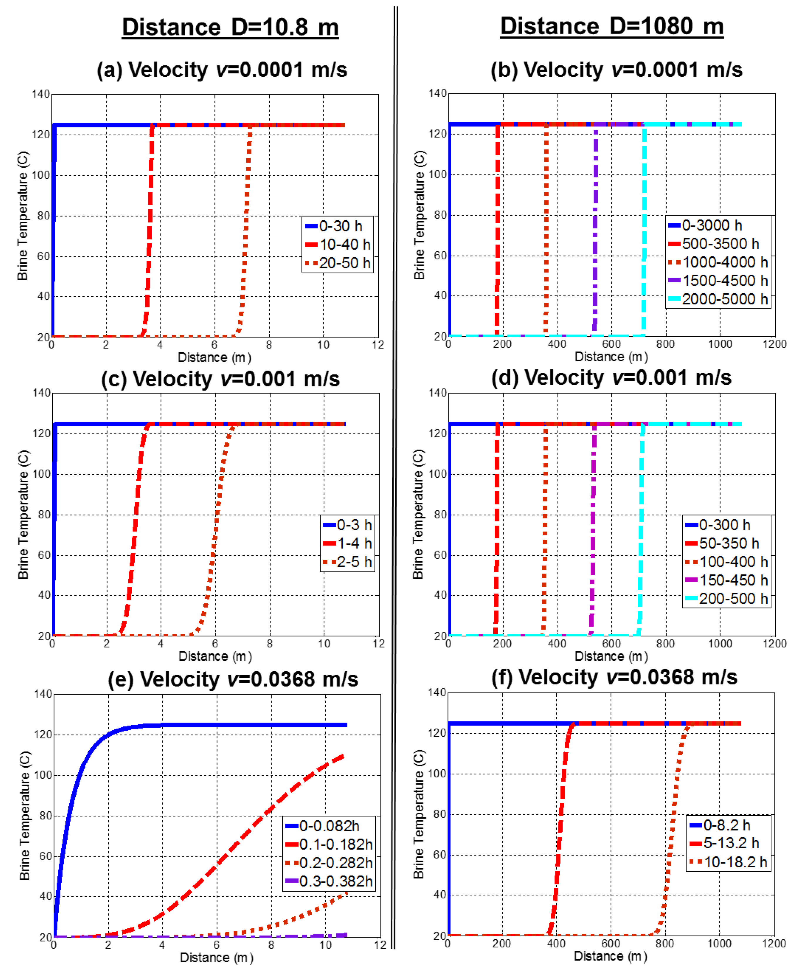
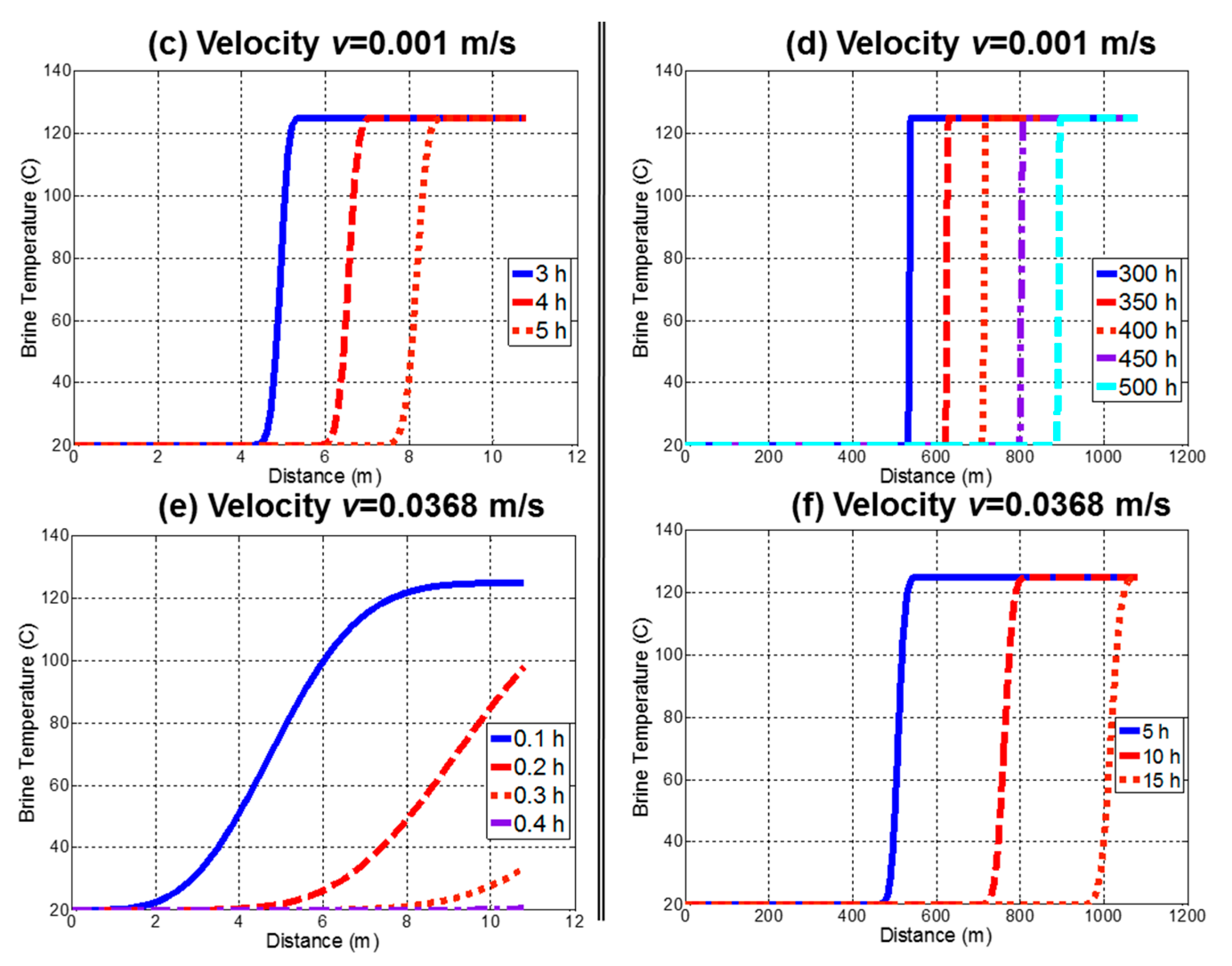
3.1. Mechanism 1: Heating of the Cold Injection Brine When Passing Along a Hotter Fracture Wall

In order to study the roles of various reservoir parameters in the process of heat transfer, the first mechanism of heat exchange (Mechanism 1, Section 2.3) is the simplest one. The fracture channel is artificially assumed to retain a constant temperature during the heat transfer to the circulating fluid.

Model Mechanism 1. Heat conduction through a channel with a uniform surface temperature T_S, of the parallel channel walls is modeled in a first assessment. The boundary condition for the brine that runs through a fracture space is a fixed temperature, which means we initially ignore the cooling effect of the brine on the channel wall rock. Figure 2 illustrates the model with the uniform surface temperature, where $T_{mi}$ is the initial brine temperature at location x = 0, and $dx$ is the distance change. Combining Newton’s law of cooling $\frac{dQ}{dt}=hA\Delta T$ and heat capacity relation $\frac{dQ}{dt}=mc\Delta T$, one can obtain the following formula for the average temperature $T_m$ along the channel [37],

$$T_m(x)=T_s+(T_{mi}-T_s)\exp \left(-\frac{P\overline{h}}{mc}x\right),\left(\mathrm{K}\right)$$

(4)

where $T_{mi}$ is the initial temperature of the brine upon entry of the fracture, $T_s$ is the temperature of the fracture wall (here first assumed constant), $P=2(L+A)$ is the perimeter of the liquid body in the fracture channel, L is the horizontal well length, and A is the fracture width, c is the heat capacity of the brine, $\overline{h}=\frac{1}{x}{\displaystyle {\int }_0^{x}h(x)dx}$, where $h(x)$ is the average heat transfer coefficient (W/(m²⋅K)), and m is the mass velocity of the liquid, which is defined as

$$m=LAv\cdot \rho .(\mathrm{kg}/\mathrm{s})$$

(5)

In this study, the heat transfer coefficient h is assumed to be constant, so that Equation (4) can be simplified to the following format:

$$T_m(x)=T_s+(T_{mi}-T_s)\exp \left(-\frac{Ph}{mc}x\right).\left(\mathrm{K}\right)$$

(6)

The temperature for any location x can be calculated according to Equation (6). We see that the unit of $\frac{L\overline{h}}{mc}x$ is dimensionless $((\frac{\mathrm{m}\cdot \mathrm{W}/({\mathrm{m}}^2\cdot \mathrm{K})}{\mathrm{k}\mathrm{g}/\mathrm{s}\cdot \mathrm{J}/(\mathrm{k}\mathrm{g}\cdot \mathrm{K})}\cdot \mathrm{m})=(-))$ so that the right-hand side of Equation (6) has unit of [K], which matches with the left-hand side. In order to calculate the heat transfer coefficient $h(x)$, the Nusselt number is introduced, defined as the ratio of convective to the conductive heat transfer across the boundary, i.e., $N_u=\frac{hA}{k}$, where $A$ is the fracture aperture, $k$ is the thermal conductivity (with unit W/(m∙K)) of the fluid, so that $h=\frac{N_{u}k}{A}$. For example, for a fully developed region for channels with uniform surface temperature, the Nusselt number is $N_u=3.657$ [37].

Inputs model Mechanism 1. We applied the model to an abandoned well pair such as typically occurs in Texas. In an extreme scenario, the initial temperature of the injection brine conforms to the local atmospheric temperature given by the seasonal temperature profile (Figure 5). The lowest monthly temperatures vary between −3.9 °C and 18.3 °C (25 °F and 65 °F in Fahrenheit), and the highest monthly temperatures range between 7.2 °C and 29 °C (45 °F and 85 °F). Based on this temperature information, the initial temperature of the injection brine is taken to be 20 °C (~70 °F), which is the average yearly atmosphere temperature of Texas.

The reservoir parameters used in our simulations are listed in

Table 1. Parameter values used for the uniform surface temperature case (Mechanism 1).

Fracture Parameters	Notation	Value	Unit
Length (of Well)	L	1000	m
Inter-well Distance	D	100–1200 m	m
Aperture	A	0.005–0.01	m
Fracture wall temperature	Ts	100/125/150 (212/257/302)	°C (°F)
Brine Parameters	Notation	Value	Unit
Initial temperature	Tmi	20 (70)	°C (°F)
Density	ρ	1	kg/m3
Heat capacity	c	4186	J/(kg·K)
Thermal conductivity	k	0.8	W/(m K)
Heat transfer coefficient	h	0.0029	W/(m2 K)
Velocity	υ	0.0001–0.0368	m/s
Nusselt number	Nu	3.657	-

. Different flow rates and reservoir apertures were used to calculate the temperature profile of the injected brine. Although well production rates for established geothermal projects range between 70 L/s (Rittershoffen [17]) and 184 L/s (Neal Hot Springs [15]), we include in our models much lower well production rates in order to explore what would be the lower limit for geothermal longevity of our fracture systems. For example, in a feasibility study of a space-conditioning system for a new campus at Texas A&M University, a production rate of just 200 m³/day is considered economically feasible (2.3 L/s [38]), which is why we include a well production rate of 1 L/s order of magnitude flow rate in our models.

In our assessment of the fluid heating profiles, we evaluated two distinct fracture apertures: 0.005 m (Base Case 1) and 0.01 m (Base Case 2). By fixing the fracture dimensions (well length and fracture aperture), we know which volumetric injection rate is associated with a particular (constant) resultant velocity for the brine in the channel. It is important to scale our results for (1) volumetric production rate from the well, which determines the practical use of the extracted heat (as argued based on the examples of Neil Hot Springs and Rittershofen (Section 1) requiring well rates in the order of 10–100 L/s for commercial applications), and (2) brine velocity in the fracture channel, which determines how much heat is picked up from the fracture walls.

To better understand what each velocity means for the effective production volume in different units,

Table 2. (a) Well rate and fracture velocity correlations for fracture aperture 0.005 m (Base Case 1). (b) Well rate and fracture velocity correlations for fracture aperture 0.01 m (Base Case 2).

(a)
Velocity (m/s)	m3/s	bbl/day	gpm	L/s
0.1	0.5	271,720	7925	500
0.0368	0.184	100,000	2917	184
0.01	0.05	27,172	793	50
0.001	0.005	2717	79	5
0.0001	0.0005	271.7	7.9	0.5
(b)
Velocity (m/s)	m3/s	bbl/day	gpm	L/s
0.1	1	543,440	15,850	1000
0.0184	0.184	100,000	2917	184
0.01	0.1	54,344	1585	100
0.001	0.01	5434	159	10
0.0001	0.001	543.4	15.9	1

Note: 1 m³/s = 543,439.65 bbl/day; 1 m³/s = 15,850.32 gpm.

a,b lists the conversion between volumetric flux values and velocity values under different unit systems. Table 2a is for fracture aperture 0.005 m (Base Case 1) and Table 2b is for fracture aperture 0.01 m (Base Case 2). The fracture length, L (Figure 4), is standardized to 1000 m.

Results Mechanism 1. The results for Base Cases 1 and 2 for various fracture surface temperatures (100 °C, 125 °C, and 150 °C) are plotted in Figure 6. The heating process of the brine was faster for smaller fracture widths and for smaller velocities, as expected, compatible with intuition. The smaller fracture width was, the faster the heating of the brine by the rock wall made an impact. The slower the brine ran, the longer it stayed in contact with the hotter fracture wall to be heated up. For example, in Figure 6b, for a brine velocity equal to 0.01 m/s, and fracture aperture of 0.005 m, with initial brine temperature 20 °C and fracture surface temperature 125 °C, the brine temperature reached 110 °C after about 1 m of travel distance toward the producer well. But for a faster brine velocity of 0.1 m/s, it took more than 8 m travel distance for the brine to reach 110 °C. The dilemma is that for lower velocities, we might reach the required brine temperature over a relatively short distance and within a short reservoir residence time, but not the required minimum economic production flux, given the finite dimensions of the assumed system (Table 1). From the experience of Neal Hot Springs, 100,000 bbl/day at 140 °C (285 °F) is an approximation limit in order to be economic for power generation [15], which corresponds to a velocity of 0.0368 m/s for fracture width 0.005 m (Base Case 1).

To highlight the influence of the reservoir aperture, another fracture aperture A = 0.01 m was used (Base Case 2), and the corresponding surface temperature and velocities were computed and plotted in Figure 6d–f. A comparison with Figure 6a–c reveals that for the smaller aperture, the brine was heated up faster. For example, comparing Figure 6a,d (other parameters are the same except the fracture aperture), the brine with velocity of 0.01 m/s only took about 1 m to reach 100 °C for Base Case 1 (Figure 6a), but Base Case 2 (Figure 6d) took 4 m to reach 100 °C. This is consistent with our intuition—because the brine volume is larger in fractures with larger apertures, it will take a longer travel distance for the brine to reach the same temperature as compared with fractures of narrower apertures.

Distance needed to reach a certain temperature. Another key result geothermal engineers may be interested in is to determine the inter-well distance (D) required for the cold brine injected at a certain rate (i.e., production volume, see Table 2a,b) to reach the target temperature. The exact distance needed to reach a certain temperature for extracted brine is calculated based on Equation (6). Assuming the surface temperature of the fracture wall remains constant, then the distance D, needed to reach a certain temperature $T_m$ is:

$$D=-\frac{Av\rho c}{h}\ln (\frac{T_m-T_s}{T_{mi}-T_s}),\left(\mathrm{m}\right)$$

(7)

where Equation (5), $m=LAv\cdot \rho$ is applied to calculate the mass flux. Using Equation (7), the brine travel distances needed to reach 90 °C (90% value of the fracture wall’s initial surface temperature 100 °C) are calculated for different velocities (and corresponding fluxes) in

Table 3. (a) Brine travel distance needed to reach 90 °C for fracture temperature 100 °C. (b) Brine travel distance needed to reach 112.5 °C for fracture temperature 125 °C. (c) Brine travel distance needed to reach 135 °C for fracture temperature 150 °C.

(a)
Fracture Aperture 0.005 m			Fracture Aperture 0.01 m
Velocity (m/s)	Flux (bbl/day)	Distance (m)	Velocity (m/s)	Flux (bbl/day)	Distance (m)
0.1	271,720	7.44	0.1	543,440	29.75
0.0368	100,000	2.74	0.0184	100,000	5.47
0.01	27,172	0.74	0.01	54,344	2.98
0.001	2717	0.07	0.001	5434	0.30
(b)
Fracture Aperture 0.005 m			Fracture Aperture 0.01 m
Velocity (m/s)	Flux (bbl/day)	Distance (m)	Velocity (m/s)	Flux (bbl/day)	Distance (m)
0.1	271,720	7.61	0.1	543,440	30.45
0.0368	100,000	2.80	0.0184	100,000	5.60
0.01	27,172	0.76	0.01	54,344	3.05
0.001	2717	0.08	0.001	5434	0.30
(c)
Fracture Aperture 0.005 m			Fracture Aperture 0.01 m
Velocity (m/s)	Flux (bbl/day)	Distance (m)	Velocity (m/s)	Flux (bbl/day)	Distance (m)
0.1	271,720	7.72	0.1	543,440	30.90
0.0368	100,000	2.84	0.0184	100,000	5.69
0.01	27,172	0.77	0.01	54,344	3.09
0.001	2717	0.08	0.001	5434	0.31

a. Similarly, the brine travel distances needed to reach 112.5 °C and 135 °C are calculated for different velocities in Table 3b,c (fracture initial temperatures of 125 and 150 °C, respectively). Table 3a–c illustrates that, if the cooling effect of the cold brine for the host rock is ignored, the brine reaches the required target temperature within 10 m travel distance along the fracture, for both Base Cases 1 and 2.

The sensitivity for fracture aperture of the travel distance needed for the brine to reach 90 °C for the 100 °C fracture temperature case is graphed in Figure 7. For a certain fracture aperture, the distance needed for the brine to reach a certain temperature increases when the velocity increases. When the brine velocity is fixed instead, the travel distance for the brine to reach a certain temperature increases when the fracture aperture increases.

3.2. Mechanism 2: Cooling of the Hot Fracture due to the Passing of a Colder Brine

In Section 3.1, the surface temperature of the fracture channel was assumed to be constant. However, in practice, the fracture surface and the adjacent rock interior will get cooled because of the heat transfer from the cold brine. In this section, the cooling effect of the fracture rock will be examined, artificially assuming the brine temperature remains constant. The temperature of the fracture wall and the adjacent rock interior will keep decreasing when additional, new volumes of cool brine are being injected, which will take away heat energy from the rock. Thus, the temperature profiles for fluid and rock are both time-dependent along the fracture channel. In this subsection, only the transient temperature profile of the fracture wall is considered. A next step (Mechanism 3) takes into account the interaction of the brine heating and simultaneous wall cooling as brine circulation time progresses (Section 2.3).

Model Mechanism 2. Assuming a certain constant velocity, the fluid will run along the distance $dx$ (Figure 4b) for each time step $dt$. For each distance segment $dx$, the fluid temperature will be denoted as $T_m^{i-1}$, and the rock temperature is $T_s^{i-1}$. For the first time step $dt$, $dx=vdt$, the fluid temperature $T_m^i$ will be calculated using Equation (6). The total heat transferred is calculated by the classical definition of heat capacity [40],

$$q_m^i=cM(T_m^i-T_m^{i-1}),\left(\mathrm{J}\right)$$

(8)

where $M$ is the mass of the brine. Next, the fracture wall rock temperature $T_s^i$ will be calculated by using the Newton’s Law of Cooling [41],

$$q_s^i=hA(T_s^i-T_m^i)\cdot dt.\left(\mathrm{J}\right)$$

(9)

Applying $q_m^i=q_s^i$ to Equations (8) and (9) we obtain:

$$T_s^i=T_m^i+q_m^i/(hAdt).\left(\mathrm{K}\right)$$

(10)

Assuming that the fracture wall surface temperature $T_s^i$ is fixed afterwards, then the temperature change along depth into the rocks interior by conductive heat transfer can be obtained using the following formula [1],

$$\frac{T-T_s^{}}{T_s^i-T_s^{}}=\mathrm{erfc}(\frac{z}{2\sqrt{\kappa t}}),(-)$$

(11)

where $\kappa$ is the thermal diffusivity, defined as $\kappa =\frac{k}{\rho c}$ (m²/s) and k (W/(m·K)) is the thermal conductivity. The temperature profile along the depth of rock measure from the fracture wall towards the rocks interior (z) is expressed as follows:

$$T(t,z)=erfc(\frac{z}{2\sqrt{\kappa t}})\cdot (T_s^i-T_s^{})+T_s^{}.\left(\mathrm{K}\right)$$

(12)

Inputs model Mechanism 2.

Table 4. Parameter values for the rock.

Rock Parameters	Notation	Value	Unit
Surface temperature	$T_s$	125 (257 °F)	°C
Density	$\rho$	2650 (quartz)	kg/m3
Heat capacity	c	710 (quartz)	J/(kg·K)
Thermal conductivity	k	1.88 (limestone)	W/(mK)
Thermal diffusivity	$\kappa$	10−6	m2/s
Heat transfer coefficient	h	0.0029	W/(m2 K)

lists the assumed parameter values for the geothermal reservoir rock, which are average values obtained from [36] and other rock mechanics publications, similar to the parameters used in [19,20]. The brine and fracture parameters used are as given in Table 1. For simplicity, in the following applications, the initial fracture surface temperatures are all assumed to be 125 °C.

Results Mechanism 2. Using Equation (12), we picked four locations along the rock wall and assumed the initial fracture surface temperature was 125 °C (inferred from the average wellbore temperature), and calculated the evolution of the rock temperature profile along the z-direction (Figure 4). The results are illustrated in Figure 8, Figure 9 and Figure 10 for velocities of 0.0001 m/s, 0.001 m/s, and 0.0368 m/s, respectively. To emphasize the temperature evolution mechanism, the location is fixed, and the temperature development with respect the time, is plotted in Figure 11, Figure 12 and Figure 13, for velocities of 0.0001 m/s, 0.001 m/s, and 0.0368 m/s, respectively. The cooling trend of the rock is clearly seen in these three figures.

Comparing Figure 8 and Figure 9, the decline profiles appear exactly the same except the locations differ in order of magnitude 10, so we will just analyze Figure 8. In Figure 8a, we see that for v = 0.0001 m/s at t = 0.01 day, the fracture wall temperature at location x = 0.002 m was still very close to a step function. The temperature changes from about 85 °C to 125 °C occurred quickly from depth 0 to 0.1 m. At t = 0.1 day, the surface temperature diffused to an even lower depth at z = 0.4 m. Then at t = 1 day, the impact of the lower temperature at the surface reached a depth z = 1 m. After that, the initial rock temperature 125 °C at depth z = 1 m started to get affected and, later, kept decreasing. Figure 8d shows that at t = 10 days, the rock temperature at depth z = 1 m was about 105 °C. For velocity v = 0.0368, the rock temperature evolution profile is plotted in Figure 13, from which we see similar process as in Figure 8 and Figure 9, but for different locations x = 0.5, 1, 2, 3 m.

Figure 11 shows a maximum cooling profile of the fracture wall. In reality, the fracture wall will cool due to the passage of cold brine, but while the interior of the rock adjacent to the fracture wall is cooling, the brine will warm up. While Mechanism 2 does not account for the coupling of brine heating (Mechanism 1) and the fracture wall cooling, Mechanism 3 does capture that process (Section 4.3).

3.3. Mechanism 3: Combination of Fluid Heating and Fracture Wall Cooling

Mechanism 1 computes the brine temperature when the fracture wall temperature is assumed to be constant, but in reality, during brine injection, the fracture wall temperature will decrease while the brine temperature increases until all heat energy is removed from the rock. During the circulation of cold brine, there are two heat transfer processes happening momentarily. One is the heat transfer between the brine and the fracture wall, and the other is the heat transfer between the fracture wall and the interior rock. The temperature profiles for fluid and rock surface are both time-dependent along the fracture channel. If we consider these two processes at the same time, the model will become extremely complicated with changing boundary conditions on the fracture wall, which are caused by the heat transfer within the rock. It is difficult to get analytical solutions for models with changing boundary conditions. To make the analytical solution possible without loss of the essential heat transfer processes, Mechanism 3 considers the cooling of the fracture wall, with the interior cooling (accounted for in Mechanism 2) excluded, and coeval heating of the circulating fluid.

Model Mechanism 3. The interaction between the cold brine and fracture wall will result in a temperature of the brine given by Equation (6), adapted with time steps,

$$T_m^i(x)=T_s^i+(T_m^{i-1}-T_s^i)\exp \left(-\frac{Ph}{mc}x\right),$$

(13)

where the value of $T_s$ is changing for each time step according to Equation (10), $T_s^i=T_m^i+q_m^i/(hAdt)$. The methodology of computing the temperature profiles is explained in Appendix A.

Results Mechanism 3. Computing the temperature of the brine based on the interaction between the rock and the fluid by using Equation (13) and the parameter values listed in Table 1 and Table 4, the fluid temperature profiles are plotted in Figure 14. Three velocities cases are chosen, v = 0.0001 m/s, 0.001 m/s, and 0.0368 m/s, and two travel distances are assumed, D = 10.8 m and D = 1080 m. In each subfigure of Figure 14, the curve specifies the brine temperature along the fracture length at a given time. For example, Figure 14a shows a blue curve for the temperature distribution along x = 0–10.8 m, at time t = 30 h after injection of the cold brine. The temperature of the brine attains the initial temperature 20 °C in the first 5 m, then it is readily heated up from 5–6 m, increasing to 125 °C.

Figure 14b,d,f shows that different velocities give different heating times for the brine. For velocity v = 0.0001 m/s (Figure 14b), it took 5000 h (about 147 days) for the brine to cool most of the fracture surface along the 1080 m total travel distance. For v = 0.001 m/s, it only took 500 h (about 15 days) to chill the fracture heat source to a surface temperature of 20 °C; for v = 0.0368 m/s (Figure 14f), the whole fracture length of 1080 m is already cooled to the original brine temperature of 20 °C after 15 h.

Based on this observation and the actual field data of the geothermal production site, economic strategies must be designed to mitigate premature cooling of the geothermal reservoir. Such a strategy will be discussed further in Section 4.2.

3.4. Mechanism 4: Recovery of the Cooled Fracture Wall by “Self-Heating"

With the continuous injection of cold brine, the fracture wall temperature will keep decreasing until the rock reaches the temperature of cold brine. When that happens, the cold brine cannot be heated by the fracture wall any more. In this section, we will study when the injection of cold brine stops, how quickly the fracture wall temperature will recover to a temperature close to the initial one, by internal heat diffusion within the rock.

Model Mechanism 4. At rock depth $z=H$, the rock has an initial temperature $T_s$, which will diffuse along the rock to the surface of the rock. The temperature profile within the rock near the fracture wall will satisfy the following set of equations:

$$\{\begin{array}{c}\frac{\partial T}{\partial t}=\kappa \frac{{\partial }^{2}T}{\partial z^2},0<z<H\\ T=\phi (z),t=0\\ T=T_1,z=0\\ \frac{\partial T}{\partial z}=0,z=H\end{array},$$

(14)

where $\kappa$ is the thermal diffusivity defined as $\kappa =\frac{k}{\rho c}$. Solving Equation (14) using separation of variables, we obtain the following solution:

$$T(z,t)={\displaystyle \sum _{n=1}^{\infty }{b}_n{e}^{-{\left(\frac{(2n-1)\pi }{2H}\right)}^2\kappa t}\sin (\frac{(2n-1)\pi }{2H}z)}+T_1,$$

(15)

where $b_n=\frac{2}{H}{\displaystyle {\int }_0^H(\phi (z)}-T_1)\sin (\frac{(2n-1)\pi }{2H}z)dz$ is the Fourier coefficient of $(\phi (z)-T_1)$. The detailed derivations are given in Appendix B, which was solved using separation of variables.

Results Mechanism 4. To investigate how fast the fracture surface temperature can recover by heat transfer from the deeper rock interior located at $H=1$ m in Equation (15), we use the initial rock temperature profile calculated by Equation (12), and plot the rock temperature profile along the depth z in Figure 15. In about five days, the temperature of the fracture surface was nearly restored to the original temperature profile. This result opens up avenues for a production plan with intermittent injection, controlled by the variables used in our analysis. For example, when the injection of cold brine has cooled the entire surface of the fracture, we can terminate the injection, and leave the abandoned well inactive for several days. The fracture surface temperature will recover to a higher temperature again by diffusion of heat stored deeper in the reservoir, away from the fracture surface.

Based on the results illustrated in Section 3.3, the increase of the brine temperature will occur more slowly as time goes because of the cooling of the fracture surface, until the brine stops to be heated when the fracture surface reaches the same low temperature as the cold brine. The continuous injection of cold brine will not be sustainable over a longer period.

4. Discussions and Intermittent Production Model

Authors should discuss the results and how they can be interpreted in perspective of previous studies and of the working hypotheses. The findings and their implications should be discussed in the broadest context possible. Future research directions may also be highlighted.

The viability of a geothermal EGS project critically hinges on three basic aspects: (1) Achieving circulation rates of a working fluid with well production rates in the range of 70 L/s to 184 L/s, (2) extracting such fluid volumes with an appropriate temperature, in the range of 100 to 150 °C, and (3) maintaining both the flux and the temperature over a 20–30 year life-cycle is essential for any commercial geothermal energy conversion project. In addition to the array of advanced numerical model platforms available for geothermal reservoir modeling (see Section 2.1), we advocate the use of reduced-order models based on analytical methods to capture the essential physics of the subterranean hydrodynamics in preliminary analyses. For example, a previous study of doublet flow between an injector and producer [42] showed that a far-field flow in a geothermal aquifer may easily lead to miscommunication and disconnection of the injection fluid and the producer well. Assuming the wells are connected by hydraulic and/or natural fractures, a flow and heat flow model of discrete fractures is more applicable for the reservoir currently studied [11].

In our present model (Figure 2), a single connected fracture plane acts as the channel for injection brine to absorb the geothermal energy, and injected brine is used as the heat transfer medium to extract the geothermal energy. Based on aspect (1), two extremely slow brine velocities, v = 0.0001 m/s and v = 0.001 m/s, and an upper limit velocity, v = 0.0368 m/s, were investigated, and correspond to fluid volumes of 0.5 L/s, 5 L/s, and 184 L/s, respectively. Following aspect (2), the fracture wall temperature is set to be 125 °C, which is the average of 100 °C and 150 °C. The main purpose of our study is to investigate aspect (3), which is the longevity of the geothermal reservoir. In the preceding sections, the corresponding heat transfer mechanisms have been modeled based on our assumption for the reservoir model, brine velocities, and rock properties.

4.1. Principle Outcomes of Simple Heat Transfer Model (Mechanisms 1–4)

Assuming the fracture wall temperature is fixed, Figure 6 illustrates the brine temperature profile under different combinations of brine velocity, fracture aperture and fracture wall temperatures (Mechanism 1). The slower the brine runs, the easier it is heated up; the smaller the fracture aperture, the easier the brine is heated up. Figure 7 shows the distances needed to reach 90 °C for the brine injected with an initial temperature of 20 °C if the fracture wall temperature is assumed at 100 °C, under different fracture apertures and velocities conditions.

In a practical situation, while the usually cooler brine is heated up by the hotter fracture wall, the wall rock will be cooled down by the brine (Mechanism 2). Figure 8, Figure 9 and Figure 10 illustrate the temperature profile of the rock interior at different times, for different locations along the fracture, for three distinct (constant) brine velocities v = 0.0001 m/s, v = 0.001 m/s, and v = 0.0368 m/s. Figure 11, Figure 12 and Figure 13 show the corresponding temperature evolution profiles at one location on the fracture wall for those velocities, which illustrate the temperature diffusion process away from the fracture wall toward the interior rock.

The mutual influence between the cold brine and hot fracture wall was considered (Mechanism 3), and the temperature profile of injection brine is plotted in Figure 14 for three different velocities, both for the shorter travel distance D = 10.8 m and longer travel distance D = 1080 m. The brine temperature profiles are different for different time steps, because of the gradual decline in the temperature of the fracture wall. For faster circulation velocities, the heat stored in the fracture wall will vanish faster. The disappearance time varies from 147 days at velocity v = 0.0001 m/s to 15 h at velocity v = 0.0368 m/s.

The fracture wall temperature drops relatively fast so that, in order to be able to continue production of brine from the fracture, the injection well needs to be switched off to let the fracture wall restore to its original temperature (Mechanism 4). Figure 15 shows that the temperature of the fracture wall will be restored to the original temperature profile relatively quickly (five days in the case considered).

4.2. Integrated Model for Longevity of Heat Extraction

Based on above insights, a sustainable and economical production plan could be proposed. The required geothermal heat for daily space conditioning, 200 m³/day (equivalent to 2.3 L/s) for a 10,000 sqft office space pilot project can be produced with just 8 h production per day. The temperature of the produced fluid, accounting for heat loss factor due to wellbore transport, was aimed to be 80–90 °C [38]. When the well is switched off after t = 8 h of hot production, the cooled fracture surface will be heated up again by conductive heat transfer from the higher temperature interior of the rock, and the fracture surface temperature will partially recover in the next 16 h, at a rate that will be specified below. The brine temperature profiles after different days under this periodic circulation plan are plotted in Figure 15.

At t = 8 h, the brine temperature and fracture wall temperature will develop the profiles shown in Figure 16a,b after applying Mechanism 3. The periodic circulation plan is repeated for day 2 until day 7 and the corresponding results are plotted in Figure 16c–h. Comparing Figure 16a–h, it is seen that the brine temperature profiles are converging to a quasi-steady state. In fact, comparing Figure 16a,c, we see that Figure 16a has two step temperatures, 20 °C and the final temperature, 125 °C, but Figure 16c has one more step temperature, which is about 85 °C and 0.7 m long. The extra step temperature is caused by the partial recovery of the fracture wall surface temperature during the 16 h recovery on the first day. The brine temperature will still be heated up to 125 °C at the end of 8 h on day 2 (Figure 16c). On day 3 (Figure 16d), another step temperature (about 110 °C) shows up in the brine temperature profile but with shorter length (0.35 m). As the production schedule continues until day 7, the same results keep showing up but the lengths of these new steps are converging to 0. The difference between Figure 16g,h is already unrecognizable in the figure scale. On day 7 (Figure 16h), the brine temperature is very close to the quasi-steady state.

To simulate the exact process of interior rock temperature change at the first 8 h, Mechanism 1 and Mechanism 2 need to be fully coupled from t = 0 to t = 8 h. In order to derive analytical solutions, we will simplify the coupling to a sequential process. The rock temperature profile after 8 h cooling given by Figure 16 will be used as the initial temperature profile for Mechanism 2. Since the actual fracture wall temperature between t = 0 to t = 8 h will be higher than the temperature at t = 8 h, this scenario will lead to the lowest possible temperature profile. Like in Figure 16, the result of Figure 17 (left column) is a faster temperature profile change as compared to a model where perfect coupling between Mechanism 1 and 2 would occur. Progressive cooling profiles for the rock interior are given in Figure 17 (left column) for the fixed velocity case, v = 0.0001 m/s. Next, the recovery of the rock interior temperature is taken into account (Mechanism 4) for the next 16 h. The result is shown in Figure 17 (right column) for the velocity v = 0.0001 m/s case.

Figure 17a clearly illustrates that, on day 1, after 8 h cooling of the rock, the first meter of the fracture length will be cooled down to as low as 20 °C, but once the circulation stops, the rock temperature, including the fracture wall temperature, will restore to about 85 °C. For example, in Figure 17a with brine velocity of v = 0.0001 m/s, after 8 h cooling the temperature of the interior of the rock is as low as 20 °C for the first 1.2 m, but after 16 h heat recovery after the injection is switched off, the temperature of the interior rock has restored to higher than 85 °C. After one day’s 8 h circulation and 16 h recovery time after switching off the pump, the rock temperature is given in Figure 17b.

This periodic circulation is repeated for day 2 to day 7, with 8 h circulation and 16 h pumps switched off, every day. The results are shown in Figure 17c–n. On day 2, after 8 h circulation, the cooling profile of the rock evolves further to x = 2 m, where the fracture wall temperature has decreased to about 80 °C. Then, after 16 h recovery in Figure 17d, the fracture rock temperature recovers, but only to 125 °C at about x = 2.15 m. On day 3, the cooled fracture portion advances further to about x = 2.5 m, but the cooling speed is slowed down. The same phenomena continue on day 4 to day 7, which leads to the quasi-steady state on day 7. The quasi-steady state distance is about x = 3 m (Figure 16h), which means for locations further than x = 3 m, the rock temperature will be always the initial rock temperature, 125 °C. The evolution of the separation lines A, B, C, and D shown in Figure 17 (left column) illustrates the convergence of the temperature profile to the quasi-steady state.

The results for velocities v = 0.001 m/s and v = 0.0368 m/s under the same conditions have also been simulated and analyzed. Quasi-steady states could still be achieved for these two velocities cases, but after longer travel distances.

4.3. Generic Insights

Our results suggest that EGS reservoirs with continuous fluid injection could quickly quench the effective transfer of heat due to rapid cooling of the fracture wall rock. The cooling advances fast along the fractures, starting from the injection point toward the producer well. A continuous circulation plan will not be able to achieve a steady state (see Appendix A), but instead will lead to fast quenching and extinction of the heat transfer process. The section that has been quenched will no longer raise the temperature of the working fluid, which is why intermittent injection is proposed to allow for recovery of the fracture wall’s temperature before the next cycle of injection fluid is circulated through the fracture system. The model presented suggests a quasi-steady state can be achieved by the intermittent fluid circulation in order to achieve a heat extraction rate that can be sustained for longer duration as required for commercial exploitation. The insight that a fractured well will cool very rapidly, we believe, is novel, and the intermittent fluid circulation is a practical solution to extend the geothermal field life, which has not been realized before. We suggest a quasi-steady state can be achieved by an appropriately proportioned intermittent circulation schedule.

4.4. Limitations of the Model

In this study, we assume that a single horizontal fracture plane connects a horizontal well pair, and the circulating brine induces various heat transfer mechanisms, modeled with a semi-analytical model. The well pair is assumed to be horizontal so that the gravity effect can be ignored, keeping the mathematical model simple. A single fracture is assumed to represent the combination of multiple shorter fractures that are more likely to exist in geothermal reservoirs. The assumption of a single fracture further simplifies the model construction and solution, while still considering all the essential heat exchange mechanisms. Cases with multiple fractures can be simulated differently with more complicated models. However, our current model can be scaled for multiple fractures, provided no geothermal energy exchange occurs between the individual fracture set. Fracture aperture and height are assumed to be uniform, so that the heat transfer model can be approximated by an analytical model description.

In our simulation, the coupling of the four heat transfer mechanisms occurs in a sequential manner, which will lead to final brine temperatures and rock temperatures that may differ from fully coupled models. In reality, all the mechanisms (Mechanisms 1–4) happen momentarily. Developing analytical solutions into a fully-coupled heat transfer model on a bounded domain is not feasible. However, even with all the limiting assumptions mentioned, the model built in this study still captures the essential mechanisms of the heat transfer process so that the results provide practical clues for management of the brine injection velocity and volume in relation to the reservoir inner temperature evolution.

The cooling of the interior rock during the injection of the cold brine is computed up to a distance 1 m away from the fracture (in a direction normal to the fracture wall), at which distance the initial temperature 125 °C is assumed constant, functioning as a deep heat source that will support the recovery of the fracture wall temperature when fluid circulation ceases. The fracture surface temperature is recharged intermittently by conductive transfer of the deeply stored heat source toward the colder fracture surface (and of the adjacent cooled interior). A quasi-steady state is achieved, because the hotter interior at a certain depth away from the fracture surface will reheat the fracture surface cooled by the circulating brine when its circulation is intermittently ceased.

5. Conclusions

Based on the assumption of channel flow for the injection brine after zip-fracking the horizontal wells, a heat transfer model was built to simulate the temperature development of the brine and the fracture wall. From the simulations of this study, the following conclusions can be drawn:

• A continuous fluid circulation in EGS reservoirs with limited fracture-matrix surface contact area will quickly quench the effective transfer of heat due to rapid cooling of the fracture wall rock. The fracture wall temperature for the region close to the injection point will equalize to the temperature of the cold injection brine in about three days in the cases studied.
• A steady-state extraction of geothermal energy cannot be achieved over longer time scales due to the rapid decline in the heat transfer rate at the fracture wall.
• A periodic circulation plan, proposed here to remedy the situation, could lead to a quasi-steady state of the extracted fluid temperature. The fracture wall is cooled by periodic injection of cold brine but will heat up fast enough after well shut-in to restore the temperature of the cooled fracture wall such that heat transfer is possible again after brine injection resumes. Our models show how fast after shut-in of the injection well the fracture rock wall interior will restore to the initial temperature.
• The temperature history of the injection brine was calculated accounting for four heat transfer mechanisms. The temperature of the cold brine requires a certain travel distance to reach a required temperature for economic production, which is scaled for the specific reservoir conditions studied here.
• The injection brine is heated faster for slower running brine and for smaller fracture aperture; however, the volumetric production is inversely proportional to the fluid velocity in the fracture space.

References

1. Turcotte, D.L.; Schubert, G. Geodynamics: Applications of Continuum Physics to Geological Problems; John Wiley & Sons: New York, NY, USA, 1982. [Google Scholar]
2. GEA Geothermal Energy Association. 2016 Annual, U.S. & Global Geothermal Power Production Report. 2016. Available online: http://www.geo-energy.org/ (accessed on 1 September 2017).
3. Electric Power Annual 2013; Independent Statistics & Analysis; U.S. Energy Information Administration: Washington, DC, USA, 2013.
4. Blackwell, D.D.; Richards, M. Geothermal Map of North America, AAPG Map, scale 1:6,500,000, Product Code 423; SMU Geothermal Laboratory: Dallas, TX, USA, 2004. [Google Scholar]
5. Williams, C.F.; Reed, M.J.; Mariner, R.H. A Review of Methods Applied by the U.S. Geological Survey in the Assessment of Identified Geothermal Resources; U.S. Department of the Interior, U.S. Geological Survey, Open-File Report 2008–1296; U.S. Department of the Interior: Washington, DC, USA, 2008; Volume 27.
6. Blackwell, D.; Richards, M.; Stepp, P. Final Report, Texas Geothermal Assessment for the I35 Corridor East; Prepared for Texas State Energy Conservation Office. Contract CM709; Southern Methodist University: Dallas, TX, USA, 29 March 2010. [Google Scholar]
7. Anderson, B.J. Recovery Act: Analysis of Low-Temperature Utilization of Geothermal Resources; Final Technical Report; Department of Energy: Washington, DC, USA.
8. NREL. Available online: http://www.nrel.gov/gis/geothermal.html (accessed on 12 April 2017).
9. Geo Explorers. Available online: www.geoexplorers.ch/eng/vision.html (accessed on 12 April 2017).
10. Fox, D.B.; Sutter, D.; Tester, J.W. The thermal spectrum of low-temperature energy use in the United States. Energy Environ. Sci. 2011, 4, 3731–3740. [Google Scholar] [CrossRef]
11. Weijermars, R.; Burnett, D.; Claridge, D.; Noynaert, S.; Pate, M.; Westphal, D.; Yu, W.; Zuo, L. Redeveloping Depleted Hydrocarbon Wells in an Enhanced Geothermal System (EGS) for s University Campus: Progress Report of a Real-Asset-Based Feasibility Study. Energy Strategy Rev. 2018, 21, 191–203. [Google Scholar] [CrossRef]
12. DOE (U.S. Department of Energy). Geothermal Technologies Program. Multi-Year Research, Development and Demonstration Plan, 2009–2015 with Program Activities to 2025, U.S., Energy Efficiency & RenewableEnergy Office. 2015. Available online: http://www.eere.energy.gov/geothermal/plans.htm. (accessed on 10 August 2017).
13. Potter, R.M.; Robison, E S.; Smith, M. Method of Extracting Heat from Dry Geothermal Reservoirs. U.S. Patent 3786858, 27 March 1972. [Google Scholar]
14. Brown, D. The US Hot Dry Rock Program-20 Years of Experience in Reservoir Testing. In Proceedings of the World Geothermal Congress, Florence, Italy, 1 January 1995. [Google Scholar]
15. Weijermars, R.; Zuo, L.; Warren, I. Modeling reservoir circulation and economic performance of the Neal Hot Springs Geothermal power plant (Oregon, U.S.): An integrated Case Study. Geothermics 2017, 70, 155–172. [Google Scholar] [CrossRef]
16. Fox, D.B.; Sutter, D.; Beckers, K.F.; Lukawski, M.J.; Koch, D.L.; Anderson, B.J.; Tester, J.W. Sustainable heat farming: Modeling extraction and recovery in discretely fractured geothermal reservoirs. Geothermics 2013, 46, 42–54. [Google Scholar] [CrossRef]
17. Baujard, C.; Genter, A.; Graff, J.J.; Maurer, V.; Dalmais, E. ECOGI, a New Deep EGS Project in Alsace, Rhine Graben, France. In Proceedings of the World Geothermal Congress 2015, Melbourne, Australia, 19–25 April 2015. [Google Scholar]
18. Vidal, J.; Genter, A.; Schmittbuhl, J. Pre-and post-stimulation characterization of geothermal well GRT-1, Rittershoffen, France: Insight form acoustic image logs of hard fractured rock. Geophys. J. Int. 2016, 845–860. [Google Scholar] [CrossRef]
19. Heuer, N.; Kupper, T.; Windelberg, D. Mathematical model of a Hot Dry Rock system. Geophys. J. Int. 1991, 105, 659–664. [Google Scholar] [CrossRef]
20. Cheng, A.H.D.; Ghassemi, A.; Detournay, E. Integral equation solution of heat extraction from a fracture in hot dry rock. Int. J. Numer. Anal. Meth. Geomech. 2001, 25, 1327–1338. [Google Scholar] [CrossRef]
21. Hori, Y.; Kitano, K.; Kaieda, H.; Kiho, K. Present status of the Ogachi HDR Project, Japan, and future plans. Geothermics 1999, 28, 637–645. [Google Scholar] [CrossRef]
22. Brown, D.W.; Duchane, D.V.; Heiken, G.; Hriscu, V.T. Mining the Earth’s Heat: Hot Dry Rock Geothermal Energy; Springer: Berlin, Germany, 2012. [Google Scholar]
23. Goldstein, R.J.; Ibele, W.E.; Patankar, S.V.; Simon, T.W.; Kuehn, T.H.; Strykowski, P.J.; Tamma, K.K.; Heberlein, J.V.R.; Davidson, J.H.; Bischof, J.; et al. Heat transfer-A review of 2005 literature. Int. J. Heat Mass Transf. 2010, 53, 4397–4447. [Google Scholar] [CrossRef]
24. Luchko, Y.; Rundell, W.; Yamamoto, M.; Zuo, L. Uniqueness and reconstruction of an unknown semilinear term in a time-fractional reaction-diffusion equation. Inverse Probl. 2013, 29, 1–17. [Google Scholar] [CrossRef]
25. Rundell, W.; Xu, X.; Zuo, L. Determination of an unknown boundary condition in a fractional diffusion equation. Appl. Anal. 2013, 92, 1511–1526. [Google Scholar] [CrossRef]
26. Luchko, Y.; Zuo, L. Theta-function method for a time-fractional reaction-diffusion equation. J. Alger. Math. Soc. 2014, 1, 1–15. [Google Scholar]
27. Moridis, G.J. A New Set of Direct and Iterative Solvers for the TOUGH2 Family of Codes; LBL Report No. 37066; USDOE: Washington, DC, USA, 1995.
28. Moridis, G.J.; Pruess, K. T2SOLV: An Enhanced Package of Solvers for the TOUGH2 Family of Codes; LBNL Report No. 39496; Lawrence Berkeley National Lab.: Berkeley, CA, USA, 1997.
29. Pruess, K.; Simmons, A.; Wu, Y.S.; Moridis, G.J. TOUGH2 Software Qualification; LBL Report No. 38383; U.S. Department of Energy: Washington, DC, USA, 1996.
30. Pruess, K.; Oldenburg, C.; Moridis, G.; Finsterle, S. Water Injection into Vapor- and Liquid-Dominated Reservoirs: Modeling of Heat Transfer and Mass Transport; LBNL Report No. 40120; USDOE: Washington, DC, USA, 1997.
31. Gringarten, A.C.; Witherspoon, P.A.; Ohnishi, Y. Theory of Heat Extraction from Fractured Hot Dry Rock. J. Geophys. Res. 1975, 80, 1120–1124. [Google Scholar] [CrossRef]
32. Martinez, A.R.; Roubinet, D.; Tartakovsky, D.M. Analytical models of heat conduction in fractured rocks. J. Geophys. Res. Solid Earth 2014, 119, 83–98. [Google Scholar] [CrossRef]
33. Fox, D.B.; Koch, D.L.; Tester, J.F. An analytical thermohydraulic model for discretely fractured geothermal reservoirs. Water Resour. Res. 2016, 52, 6792–6817. [Google Scholar] [CrossRef]
34. Hawkins, A.J.; Becker, M.W.; Tsoflias, P.T. Evaluation of inert tracers in a bedrock fracture using ground penetrating radar and thermal sensors. Geothermics 2017, 67, 86–94. [Google Scholar] [CrossRef]
35. Blackwell, D.; Richards, M.C.; Frone, Z.S.; Batir, J.F.; Williams, M.A.; Ruzo, A.A.; Dingwall, R.K. SMU Geothermal Laboratory Heat Flow Map of the Conterminous United States; SMU Geothermal Laboratory: Dallas, TX, USA, 2011. [Google Scholar]
36. Jaeger, J.C.; Cook, N.G.; Zimmerman, R. Fundamentals of Rock Mechanics, 4th ed.; Wiley-Blackwell: Oxford, UK, 2007; ISBN 978-0-632-05759-7. [Google Scholar]
37. Jiji, L.M. Heat Convection; Springer: Berlin/Heidelberg, Germany, 2006. [Google Scholar]
38. Westphal, D.; Weijermars, R. Economic Appraisal and Scoping of Geothermal Enrgy Extraction Projects using Depleted Hydrocarbon Wells. Energy Strategy Rev. 2018, 22, 348–364. [Google Scholar] [CrossRef]
39. USclimatedata. Available online: http://www.usclimatedata.com/climate/texas/united-states/3213 (accessed on 19 July 2017).
40. Rohsenow, W.M.; Hartnett, J.P.; Cho, Y.I. Handbook of Heat Transfer, 3rd ed.; McGraw-Hill: New York, NY, USA, 1998. [Google Scholar]
41. Burmeister, L.C. Convective Heat Transfer, 2nd ed.; Wiley-Interscience: Hoboken, NJ, USA, 1993; p. 107. ISBN 0-471-57709-X, 9780471577096. [Google Scholar]
42. Weijermars, R.; van Harmelen, A. Breakdown of doublet re-circulation and direct line drives by far-field flow: Implications for geothermal and hydrocarbon well placement. Geophys. J. Int. 2016, 206, 19–47. [Google Scholar] [CrossRef]
Figure 1. Geothermal resource distribution and geothermal resource extraction methods. (a) Geothermal resource map of the United States (Reproduced with permission from [8]), with the dotted region outlining identified hydrothermal sites. Color coding classifies favorability to enhanced geothermal systems (EGS) systems. (b) Relative depth and temperature range (°C) of different heat extraction methods (Reproduced with permission from [9]).
Fluids 04 00063 g001
Figure 2. Schematic of abandoned hydrocarbon horizontal well system in terms of the corresponding physical model. (a) System comprises two horizontal wells connected by a single fracture plane. (b) Zoom in of the heat flow model within the fracture channel.
Fluids 04 00063 g002
Figure 3. Illustration of the heat transfer system with geothermal heat flux from below. Fluid is injected from the left side of the system.
Fluids 04 00063 g003
Figure 4. Fracture surface temperature increases over time due to heat flux. (a) Temperature profile at the fracture surface with respect to time, in year; (b) Temperature profile with respect to rock depth at fixed time t = 5 years, with z = −100 m as the depth of the uniformly applied geothermal heat flux. In both figures, the initial temperature of the fracture wall rock is T 0 = 20 °C, heat flux q f = 0.06 W/m2, thermal conductivity k = 1.88 W/(m∙K)(Limestone value from [36]), thermal diffusivity is κ = 10−6 m2/s, and the total rock depth is 100 m.
Fluids 04 00063 g004
Figure 5. Texas climograph data in 2016. The blue line is the average low temperature of each month, and the red line is the average high temperature of each month. The blue bars give the relative average monthly precipitation (Reproduced with permission from [39]).
Fluids 04 00063 g005
Figure 6. Temperature profiles for various injection flow rates when surface temperature of the fracture wall rock is 100 °C, 125 °C, and 150 °C for Base Case 1 and Base Case 2, and the total flow rate at the producer wells is between 0.005 m3/s to 0.5 m3/s. Fracture apertures and surface temperatures are (a) 0.005 m, 100 °C; (b) 0.005 m, 125 °C; (c) 0.005 m, 150 °C; (d) 0.01 m, 100 °C; (e) 0.01 m, 125 °C; (f) 0.01 m, 150 °C.
Fluids 04 00063 g006
Figure 7. Sensitivity of travel distance and fracture aperture required to reach the target brine temperature of 90 °C (assuming fracture surface temperature fixed at 100 °C) for various brine velocities.
Fluids 04 00063 g007
Figure 8. Cooling profile of the host rock at four locations (x = [0.002, 0.004, 0.008, 0.012] (m)) for different times. (a) t = 0.01 day; (b) t = 0.1 day; (c) t = 1 day; (d) t = 10 days. Initial rock temperature is 125 °C. Fracture aperture is 0.005 m. Brine velocity is 0.0001 m/s. The initial fracture wall temperature for time 0 is defined when first fresh injected fluid batch passes by. For example, for x = 0.002 m, the reference time is 0.002/0.0001 = 20 s.
Fluids 04 00063 g008
Figure 9. Cooling profile of the host rock at four locations (x = [0.02, 0.04, 0.08, 0.12] (m)) for different times. (a) t = 0.01 day; (b) t = 0.1 day; (c) t = 1 day; (d) t = 10 days. Initial rock temperature is 125 °C. Fracture aperture is 0.005 m. Brine velocity is 0.001 m/s. The initial fracture wall temperature for time 0 is defined when first fresh injected fluid batch passes by. For example, for x = 0.002 m, the reference time is 0.02/0.001 = 20 s.
Fluids 04 00063 g009
Figure 10. Cooling profile of the host rock at four locations (x = [0.5, 1, 2, 3] (m)) for different times. (a) t = 0.01 day; (b) t = 0.1 day; (c) t = 1 day; (d) t = 10 days. Initial rock temperature is 125 °C. Fracture aperture is 0.005 m. Brine velocity is 0.0368 m/s. The initial fracture wall temperature for time 0 is defined when first fresh injected fluid batch passes by. For example, for x = 0.002 m, the reference time is 0.5/0.0368 = 13.6 s.
Fluids 04 00063 g010
Figure 11. Cooling profile of the rock wall at x = 0.004 m for four different times: 0.01, 0.1, 1, and 10 days. Initial rock temperature is 125 °C. Fracture aperture is 0.005 m. Brine velocity is 0.0001 m/s.
Fluids 04 00063 g011
Figure 12. Cooling profile of the rock wall at x = 0.04 m for four different times: 0.01, 0.1, 1, and 10 days. Initial rock temperature is 125 °C. Fracture aperture is 0.005 m. Brine velocity is 0.001 m/s.
Fluids 04 00063 g012
Figure 13. Cooling profile of the rock wall at x = 0.5 m for four different times: 0.01, 0.1, 1, and 10 days. Initial rock temperature is 125 °C. Fracture aperture is 0.005 m. Brine velocity is 0.0368 m/s.
Fluids 04 00063 g013
Figure 14. Brine temperature profiles at different distances from the injection point in the fracture. The short-term (left) and long-term (right) heating profiles are shown for three different velocities. (a,b) v = 0.0001 m/s, (c,d) v = 0.001 m/s, and (e,f) 0.0368 m/s.
Fluids 04 00063 g014aFluids 04 00063 g014b
Figure 15. Fracture wall temperature heat recovery profile for x = 0.5 m, and five different time steps given in the legend. The initial rock temperature profile is the same as Figure 10b, which is the rock interior temperature profile after t = 0.1 day, velocity = 0.0368 m/s.
Fluids 04 00063 g015
Figure 16. Brine temperature profiles (subfigures a,ch) and fracture wall temperature profile (subfigure b) after 8 h on different days, for brine velocity = 0.0001 m/s. (a) Day 1; (b) day 1; (c) day 2; (d) day 3; (e) day 4; (f) day 5; (g) day 6; (h) day 7.
Fluids 04 00063 g016
Figure 17. Illustration of the rock temperature evolution profiles after different days. Brine velocity v = 0.0001 m/s, initial brine temperature is 20 °C, and initial rock temperature is 125 °C. (a) Day 1, after 8 h brine circulation; (b) day 1, after 16 h flow stagnation/recovery; Same on–off circulation schedule for day 2 (c,d), day 3 (e,f), day 4 (g,h), day 5 (i,j) day 6 (k,l), day 7 (m,n).
Fluids 04 00063 g017aFluids 04 00063 g017b