Lubrication Approximation for Fluids with Shear-Dependent Viscosity

Abstract

We present dimensionally reduced Reynolds type equations for steady lubricating flows of incompressible non-Newtonian fluids with shear-dependent viscosity by employing a rigorous perturbation analysis on the governing equations of motion. Our analysis shows that, depending on the strength of the power-law character of the fluid, the novel equation can either present itself as a higher-order correction to the classical Reynolds equation or as a completely new nonlinear Reynolds type equation. Both equations are applied to two classic problems: the flow between a rolling rigid cylinder and a rigid plane and the flow in an eccentric journal bearing.

1. Introduction

The Reynolds’ lubrication approximation (Reynolds [1]) of the Navier-Stokes equation is a cornerstone of classical fluid mechanics. This approximation has tremendous value as it is relevant to many technological applications. However, many of the lubricating oils that are currently in use cannot be appropriately described by the Navier-Stokes constitutive theory. Many of the lubricating oils exhibit a variety of departures from Newtonian behavior, they shear thin, display stress-relaxation, instantaneous elasticity, non-linear creep, threshold for the strain rate before they start to flow, thixotropy, etc. Many constitutive models of the differential, rate and integral type have been developed to describe the non-Newtonian behavior exhibited by such fluids, and lubricating approximations have been derived for a variety of fluid flows governed by these equations. In this paper, we are only interested in a very special sub-class of non-Newtonian fluids, namely we are interested in developing a lubrication approximation for shear thinning fluids.

We do not aim to provide an exhaustive review of the numerous studies that have been carried out to simplify and approximate the governing equations that arise from assuming different non-Newtonian characteristics, a more complete list of the same can be found in the papers that we mention below. We merely cite some representative papers that consider the different departures from classical Newtonian behavior and in which the lubrication approximation has been developed. A discussion of several of the studies that have been carried out can be found in the book by Szeri [2], see also [3,4,5]. Early studies concerning the lubrication approximation for the flow of power-law constitutive relations were primarily concerned with purely one dimensional flows where inertial effects do not manifest themselves (see for instance Shukla et al. [6]); others concern non-inertial flows (see for example Park and Kwon [7]), and yet others concern the lubrication approximation for a power law fluid, under infinite wide gap approximation (see the study by Johnson and Mangkoesoebroto [8]). Bourgin [9], see also Kacou et al. [10], developed lubrication approximation for fluids of the differential type and Harnoy [11] studied the lubrication approximation for an elastic-viscous fluid in a short journal bearing. Ballal and Rivlin [12] studied the flow of a viscoelastic fluid in a journal bearing using a perturbation analysis which was shown to be incorrect by San Andres and Szeri [13]. Cal et al. [14] developed a lubrication approximation for viscoelastic fluids and showed that viscoelasticity can have pronounced effect for certain values of the film thickness and in the case of the journal bearing, the eccentricity. Also, in flows involving high pressures as encountered in elastohydrodynamics, the pressure dependence of viscosity has to be taken into account (see Barus [15], Bair [16]). Lubrication approximation has been developed in the case of fluids with pressure dependent viscosity by Rajagopal and Szeri [17] and Gustafsson et al. [18]. Finally, Fusi et al. [19] have studied the lubrication approximation for a Bingham fluid taking into account inertial effects; fluids like the Bingham fluid that have a threshold in the stress for flow to take place are best described by constitutive relations wherein the kinematics is described as a function of the stress rather than expressing the stress in terms of the kinematical variable in the traditional manner (see Rajagopal [20,21] for a discussion of such fluids as well as more general fluids that are described by implicit constitutive relations). As there is a threshold for the stress beyond which the fluid starts to flow, the governing equations are quite different from the lubrication approximation obtained in the case of the other studies that employ fluid models that do not have such a threshold for the flow to take place.

The current study that is being carried out takes into consideration nonlinearities both due to the shear dependent viscosity and inertia and the flow is two dimensional. Although the inertial effects are not omitted a priori they do not influence the flow characteristics at the orders of approximation considered in this work (see Nazarov and Videman [22] for the inertial correction to the Reynolds lubrication approximation). The power-law fluid model under consideration has two constants that determine its viscosity, a constant power-law exponent n and another constant ${\alpha }_0$ that determines the departure of the viscosity from the Newtonian viscosity when the power-law exponent is 2 (see Equation (7)). A formal perturbation analysis is carried out, assuming two different possibilities for the material parameter ${\alpha }_0$, namely that it is of the order $\mathcal{O}\left({ϵ}^3\right)$ and $\mathcal{O}\left({ϵ}^2\right)$, and new lubrication approximations are derived. In the former case, we simply obtain a higher-oder correction to the classical (linear) Reynolds equation but if ${\alpha }_0$ is of $\mathcal{O}\left({ϵ}^2\right)$ the Reynolds type equation becomes fully nonlinear and must be solved together with an ODE for the main part of the flow velocity. Using these approximations, two problems are solved, the first being the fluid flow between a rolling rigid cylinder and a rigid plane, and the second being the problem of the fluid flowing in an eccentric journal bearing

2. Formulation of the Problem

Consider the following set of partial differential equations governing the isothermal flow of an incompressible, homogeneous power-law fluid

$$\begin{array}{cc}\hfill {\displaystyle \rho \left(\frac{\partial \mathbf{v}}{\partial t}+[\nabla \mathbf{v}]\mathbf{v}\right)+\nabla p}& =\rho \mathbf{f}+\mathrm{div}\mathbf{S},\hfill \end{array}$$

(1)

$$\begin{array}{cc}\hfill \mathrm{div}\mathbf{v}& =0,\hfill \end{array}$$

(2)

where $\rho >0$ is the constant density of the fluid, $\mathbf{v}=(u,v)$ is the velocity field, $\mathbf{S}$ is the deviatoric stress tensor ($\mathbf{T}=-p\mathbf{I}+\mathbf{S}$ is the Cauchy stress tensor), p is a scalar variable, often referred to as the mechanical pressure, associated with the incompressibility constraint (2), and $\mathbf{f}$ is an external force acting on the fluid. Whether p is the mean value of the stress depends on the constitutive relationship for the extra stress tensor S. In general, p is not the mean value of the stress but for the model considered in this paper it is (see Rajagopal [23] for a detailed discussion of the notion of pressure, its use, misuse and abuse). The deviatoric stress tensor for a fluid with shear-dependent viscosity which we shall study is related to the symmetric part of the velocity gradient as follows:

$$\mathbf{S}=2{\mu }_0{\left(1+{\alpha }_0{\left|\mathbf{D}\right|}^2\right)}^{\frac{n-2}{2}}\mathbf{D},$$

(3)

where $n\ge 1$ is the power-law exponent and ${\alpha }_0$ a scalar coefficient related to the power-law character of the fluid, with dimensions of time squared ($\dim \left[{\alpha }_0\right]=T^2$). Moreover, $\mathbf{D}\left(\mathbf{v}\right)=\frac{1}{2}\left(\nabla \mathbf{v}+{(\nabla \mathbf{v})}^T\right)$ denotes the symmetric part of the velocity gradient ${(\nabla \mathbf{v})}_{ij}=\frac{\partial v_i}{\partial x_j}$, and ${\mu }_0>0$ is a constant.

2.1. Lubrication Approximation

Let us restrict our attention to steady two-dimensional thin flows without external forces ($\mathbf{f}=0$). We will now introduce the following dimensionless (starred) quantities

$$(x^{*},y^{*})=L^{-1}(x,y),{\mathbf{v}}^{*}=U^{-1}\mathbf{v},p^{*}=P^{-1}p,{\mathbf{S}}^{*}=S^{-1}\mathbf{S},{\alpha }_0^{*}=U^2{L}^{-2}{\alpha }_0,$$

(4)

where L and U represent typical length and velocity scales and where the characteristic pressure P and the characteristic stress S are taken to be

$$P=S={\mu }_{0}U{L}^{-1}.$$

(5)

We will define the usual Reynolds number $\mathrm{Re}$ through

$$\mathrm{Re}=\rho UL{\mu }_0^{-1},$$

(6)

and make the following assumptions that are appropriate for a class of lubrication problems:

• the flow takes place between two almost parallel surfaces situated at $y=0$ and $y=H\left(x\right)$;
• the lubricating film is thin, that is, $H\left(x\right)=ϵh\left(x\right)$, where $ϵ\ll 1$ denotes a small non-dimensional parameter;
• the flow is slow enough or the viscosity high enough so that $\mathrm{Re}=\mathcal{O}\left(ϵ\right)$;
• the power-law parameter will have to be such that ${\alpha }_0=\mathcal{O}\left({ϵ}^2\right)$ or ${\alpha }_0=\mathcal{O}\left({ϵ}^3\right)$.

Next, we will drop the stars and introduce the fast variable $y\to {ϵ}^{-1}y$ (the stretched normal coordinate). The equations then become

$$\begin{array}{cc}\hfill {\displaystyle \mathrm{Re}\left([\nabla \mathbf{v}]\mathbf{v}\right)+\nabla p}& =2\mathrm{div}\left\{{\left(1+{\alpha }_0{\left|\mathbf{D}\right|}^2\right)}^{\frac{n-2}{2}}\mathbf{D}\right\},\hfill \end{array}$$

(7)

$$\begin{array}{cc}\hfill \mathrm{div}\mathbf{v}& =0.\hfill \end{array}$$

(8)

The adherence boundary conditions on rigid, impermeable boundaries read as

$$\begin{array}{cc}\hfill \mathbf{v}={\mathbf{U}}^0,{\mathbf{U}}^0·{\mathbf{e}}_y=0,{\mathbf{U}}^0·{\mathbf{e}}_x=U^0,\mathrm{at}y& =0,\hfill \end{array}$$

(9)

$$\begin{array}{cc}\hfill \mathbf{v}={\mathbf{U}}^h,{\mathbf{U}}^h·{\mathbf{e}}_{\nu }=0,{\mathbf{U}}^0·{\mathbf{e}}_{\tau }=U^h,\mathrm{at}y& =h\left(x\right),\hfill \end{array}$$

(10)

where ${\mathbf{U}}^0$ and ${\mathbf{U}}^h$ denote given constant velocities of the boundaries and ${\mathbf{e}}_{\nu }$ and ${\mathbf{e}}_{\tau }$ stand for the unit normal and tangent vectors at $y=h\left(x\right)$. These vectors are related to the unit vectors ${\mathbf{e}}_x$ and ${\mathbf{e}}_y$ through the formulae

$$\begin{array}{cc}\hfill {\mathbf{e}}_{\nu }& =\frac{\nabla \left(ϵh\right(x)-y)}{\parallel \nabla \left(ϵh\right(x)-y)\parallel }=\frac{\frac{\partial }{\partial x}(ϵh\left(x\right)-y){\mathbf{e}}_x+\frac{\partial }{\partial y}(ϵh\left(x\right)-y){\mathbf{e}}_y}{\sqrt{1+{ϵ}^2{\left(h^{\prime }\left(x\right)\right)}^2}}=\frac{ϵh^{\prime }\left(x\right){\mathbf{e}}_x-{\mathbf{e}}_y}{\sqrt{1+{ϵ}^2{\left(h^{\prime }\left(x\right)\right)}^2}},\hfill \end{array}$$

(11)

$$\begin{array}{cc}\hfill {\mathbf{e}}_{\tau }& =\frac{{\mathbf{e}}_x+ϵh^{\prime }\left(x\right){\mathbf{e}}_y}{\sqrt{1+{ϵ}^2{\left(h^{\prime }\left(x\right)\right)}^2}}.\hfill \end{array}$$

(12)

2.2. Formal Asymptotic Analysis

2.2.1. Case ${\alpha }_0=\mathcal{O}\left({ϵ}^3\right)$

We will assume the following ansatz

$$\begin{array}{cc}\hfill \mathbf{v}(ϵ,\mathbf{x})& ={ϵ}^0{\mathbf{v}}^{\left(1\right)}\left(\mathbf{x}\right)+{ϵ}^1{\mathbf{v}}^{\left(2\right)}\left(\mathbf{x}\right)+{ϵ}^2{\mathbf{v}}^{\left(3\right)}\left(\mathbf{x}\right)+\dots ,\hfill \end{array}$$

(13)

$$\begin{array}{cc}\hfill p(ϵ,\mathbf{x})& ={ϵ}^{-2}{p}^{\left(0\right)}\left(s\right)+{ϵ}^{-1}{p}^{\left(1\right)}\left(\mathbf{x}\right)+{ϵ}^0{p}^{\left(2\right)}\left(\mathbf{x}\right)+{ϵ}^1{p}^{\left(3\right)}\left(\mathbf{x}\right)+\dots ,\hfill \end{array}$$

(14)

where $\mathbf{x}=(x,y)$ and the functions ${\mathbf{v}}^{\left(\mathrm{j}\right)},p^{\left(\mathrm{j}\right)}$ and are of $\mathcal{O}\left(1\right)$. According to the assumptions $\mathrm{Re}=\mathcal{O}\left(ϵ\right)$ and ${\alpha }_0=\mathcal{O}\left({ϵ}^3\right)$, and thus on setting

$$\mathrm{Re}=ϵ\mathcal{R},{\alpha }_0={ϵ}^3\alpha ,$$

(15)

we obtain $\mathcal{R}$ and $\alpha$ are of order one.

Inserting the asymptotic expansions (13) and (14) into Equations (7) and (8), we obtain at $\mathcal{O}\left({ϵ}^{-3}\right)$ in (1) that $p^{\left(0\right)}=p^{\left(0\right)}\left(x\right)$, i.e., independent of y; at $\mathcal{O}\left({ϵ}^{-2}\right)$ in (1), at $\mathcal{O}\left({ϵ}^{-1}\right)$ in (2) and at $\mathcal{O}\left({ϵ}^0\right)$ in (9) and (10)

$$\begin{array}{cc}\hfill {\displaystyle \frac{\mathrm{d}{p}^{\left(0\right)}}{\mathrm{d}x}}& =\frac{{\partial }^2{u}^{\left(1\right)}}{\partial y^2},\hfill \end{array}$$

(16)

$$\begin{array}{cc}\hfill {\displaystyle \frac{\partial p^{\left(1\right)}}{\partial y}}& =0,\hfill \end{array}$$

(17)

$$\begin{array}{cc}\hfill \frac{\partial v^{\left(1\right)}}{\partial y}& =0,\hfill \end{array}$$

(18)

$$\begin{array}{cc}\hfill u^{\left(1\right)}=U^0,v^{\left(1\right)}& =0,\mathrm{at}y=0,\hfill \end{array}$$

(19)

$$\begin{array}{cc}\hfill u^{\left(1\right)}=U^h,v^{\left(1\right)}& =0,\mathrm{at}y=h\left(x\right),\hfill \end{array}$$

(20)

where $U^0$ and $U^h$ denote the tangential velocities at $y=0$ and at $y=h\left(x\right)$.

From (18)–(20) it follows that

$$v^{\left(1\right)}(x,y)\equiv 0.$$

(21)

We have moreover that $p^{\left(1\right)}=p^{\left(1\right)}\left(x\right)$ from (17). Using Equation (16) and the boundary conditions (19) and (20) for $u^{\left(1\right)}$ we conclude that

$$u^{\left(1\right)}(x,y)=U^0+\frac{U^h-U^0}{h\left(x\right)}y+\frac{y(y-h(x\left)\right)}{2}\frac{\mathrm{d}{p}^{\left(0\right)}}{\mathrm{d}x}.$$

(22)

The equations at the next order read as

$$\begin{array}{cc}\hfill \frac{\mathrm{d}{p}^{\left(1\right)}}{\mathrm{d}x}& =\frac{1}{2}\left[\frac{1}{2}(n-4)\alpha {\left(\frac{\partial u^{\left(1\right)}}{\partial y}\right)}^2\frac{{\partial }^2{u}^{\left(1\right)}}{\partial y^2}+(n-2)\alpha {\left(\frac{\partial u^{\left(1\right)}}{\partial y}\right)}^2\frac{{\partial }^2{u}^{\left(1\right)}}{\partial y^2}\right.\hfill \\ & \left.+\alpha {\left(\frac{\partial u^{\left(1\right)}}{\partial y}\right)}^2\frac{{\partial }^2{u}^{\left(1\right)}}{\partial y^2}+2\frac{{\partial }^2{u}^{\left(2\right)}}{\partial y^2}\right],\hfill \end{array}$$

(23)

$$\begin{array}{cc}\hfill \frac{\partial p^{\left(2\right)}}{\partial y}& =-\frac{{\partial }^2{u}^{\left(1\right)}}{\partial x\partial y},\hfill \end{array}$$

(24)

$$\begin{array}{cc}\hfill \frac{\partial v^{\left(2\right)}}{\partial y}& =-\frac{\partial u^{\left(1\right)}}{\partial x}\hfill \end{array}$$

(25)

$$\begin{array}{cc}\hfill v^{\left(2\right)}& =u^{\left(2\right)}=0,\mathrm{at}y=0,\hfill \end{array}$$

(26)

$$\begin{array}{cc}\hfill v^{\left(2\right)}& =U^h{h}^{\prime }\left(x\right),u^{\left(2\right)}=0\mathrm{at}y=h\left(x\right).\hfill \end{array}$$

(27)

Equations (24)–(27) can be expressed as a one-dimensional Stokes system for $(v^{\left(2\right)},p^{\left(2\right)})$. Assuming that this system is solvable, it follows from (23) and (25) that $u^{\left(2\right)}$ satisfies the second-order ODE (in y)

$$\begin{array}{cc}\hfill \frac{{\partial }^2{u}^{\left(2\right)}}{\partial y^2}& =\frac{\mathrm{d}{p}^{\left(1\right)}}{\mathrm{d}x}-\frac{3}{4}(n-2)\alpha {\left(\frac{\partial u^{\left(1\right)}}{\partial y}\right)}^2\frac{{\partial }^2{u}^{\left(1\right)}}{\partial y^2}\hfill \end{array}$$

(28)

$$\begin{array}{cc}\hfill u^{\left(2\right)}& =0,\mathrm{at}y=0,\hfill \end{array}$$

(29)

$$\begin{array}{cc}\hfill u^{\left(2\right)}& =0,\mathrm{at}y=h\left(x\right).\hfill \end{array}$$

(30)

On the other hand, the Stokes system (24)–(27) is solvable if and only if the compatibility condition

$${\int }_0^{h\left(x\right)}{\displaystyle \frac{\partial u^{\left(1\right)}}{\partial x}}\mathrm{d}y=-h^{\prime }\left(x\right)U^h$$

(31)

is satisfied. Using the Leibniz rule, this amounts to

$$\frac{\mathrm{d}}{\mathrm{d}x}{\int }_0^{h\left(x\right)}{u}^{\left(1\right)}\mathrm{d}y=0,$$

(32)

The classical Reynolds equation for $p^{\left(0\right)}$ is then a consequence of (22), namely

$${\displaystyle \frac{\mathrm{d}}{\mathrm{d}x}}\left[{\displaystyle \frac{h^3}{12}}{\displaystyle \frac{\mathrm{d}{p}^{\left(0\right)}}{\mathrm{d}x}}\right]={\displaystyle \frac{1}{2}}{\displaystyle \frac{\mathrm{d}h}{\mathrm{d}x}}(U^0+U^h).$$

(33)

The equations at $\mathcal{O}\left({ϵ}^0\right)$ in (1), at $\mathcal{O}\left({ϵ}^1\right)$ in (2) and at $\mathcal{O}\left({ϵ}^2\right)$ in (9) and (10) read as

$$\begin{array}{cc}\hfill \frac{{\partial }^2{u}^{\left(3\right)}}{\partial y^2}& =\dots ,\hfill \end{array}$$

(34)

$$\begin{array}{cc}\hfill {\displaystyle \frac{\partial p^{\left(3\right)}}{\partial y}+\frac{{\partial }^2{v}^{\left(3\right)}}{\partial y^2}}& =\dots ,\hfill \end{array}$$

(35)

$$\begin{array}{cc}\hfill \frac{\partial v^{\left(3\right)}}{\partial y}& =-\frac{\partial u^{\left(2\right)}}{\partial x},\hfill \end{array}$$

(36)

$$\begin{array}{cc}\hfill u^{\left(3\right)}& =v^{\left(3\right)}=0,\mathrm{at}y=0,\hfill \end{array}$$

(37)

$$\begin{array}{cc}\hfill u^{\left(3\right)}& =-{\displaystyle \frac{1}{2}}{h}^{\prime 2}{U}^h,v^{\left(3\right)}=0,\mathrm{at}y=h\left(x\right),\hfill \end{array}$$

(38)

where by … we have denoted terms which are known from the previous equations and are thus irrelevant for the following computations.

Equations (35)–(38) form a one-dimensional Stokes system for $(v^{\left(3\right)},p^{\left(3\right)})$ and the velocity component $u^{\left(3\right)}$ satisfies the second-order ODE

$$\begin{array}{cc}\hfill \frac{{\partial }^2{u}^{\left(3\right)}}{\partial y^2}& =\dots ,\hfill \end{array}$$

(39)

$$\begin{array}{cc}\hfill u^{\left(3\right)}& =0,\mathrm{at}y=0,\hfill \end{array}$$

(40)

$$\begin{array}{cc}\hfill u^{\left(3\right)}& =-{\displaystyle \frac{1}{2}}{h}^{\prime 2}{U}^h,\mathrm{at}y=h\left(x\right).\hfill \end{array}$$

(41)

arising from Equation (34) and from the boundary conditions (37) and (38). Recall that terms indicated by … have already been determined by the lower order equations.

The one-dimensional Stokes system for $(v^{\left(3\right)},p^{\left(3\right)})$ is solvable if and only if the following compatibility condition is satisfied

$${\int }_0^{h\left(x\right)}{\displaystyle \frac{\partial u^{\left(2\right)}}{\partial x}}\mathrm{d}y=0.$$

(42)

Using the Leibniz integral rule, this condition becomes

$$\frac{\mathrm{d}}{\mathrm{d}x}{\int }_0^{h\left(x\right)}{u}^{\left(2\right)}\mathrm{d}y=0.$$

(43)

Integrating by parts, one sees that

$${\int }_0^{h\left(x\right)}{u}^{\left(2\right)}\mathrm{d}y=\frac{1}{2}{\int }_0^{h\left(x\right)}y\left(y-h\left(x\right)\right){\displaystyle \frac{{\partial }^2{u}^{\left(2\right)}}{\partial y^2}}\mathrm{d}y.$$

(44)

Substituting (28) into the previous expression leads to a Reynolds type equation for the first-order pressure correction

$$\begin{array}{cc}\hfill \frac{\mathrm{d}}{\mathrm{d}x}\left[{\displaystyle \frac{h^3}{12}}{\displaystyle \frac{\mathrm{d}{p}^{\left(1\right)}}{\mathrm{d}x}}\right]& =\frac{\alpha (n-2)}{320}\left[5h^{\prime }{\displaystyle \frac{\mathrm{d}{p}^{\left(0\right)}}{\mathrm{d}x}}\left(4{(U^h-U^0)}^2+h^4{\left({\displaystyle \frac{\mathrm{d}{p}^{\left(0\right)}}{\mathrm{d}x}}\right)}^2\right)\right.\hfill \\ & +\left.h{\displaystyle \frac{{\mathrm{d}}^2{p}^{\left(0\right)}}{\mathrm{d}{x}^2}}\left(20{(U^h-U^0)}^2+3h^4{\left({\displaystyle \frac{\mathrm{d}{p}^{\left(0\right)}}{\mathrm{d}x}}\right)}^2\right)\right].\hfill \end{array}$$

(45)

2.2.2. Case ${\alpha }_0=\mathcal{O}\left({ϵ}^2\right)$

Using again the ansatz (13) and (14) and making the same assumptions as in the previous case, except for the material parameter ${\alpha }_0$ which is written as ${\alpha }_0=\alpha {ϵ}^2$, we obtain at $\mathcal{O}\left({ϵ}^{-3}\right)$ in (1) that ${\displaystyle \frac{\partial p^{\left(0\right)}}{\partial y}}=0$, i.e., $p^{\left(0\right)}$ is independent of y.

At $\mathcal{O}\left({ϵ}^{-2}\right)$ in (1), at $\mathcal{O}\left({ϵ}^{-1}\right)$ in (2) and at $\mathcal{O}\left({ϵ}^0\right)$ in (9) and (10), we obtain, respectively

$$\begin{array}{cc}\hfill {\displaystyle \frac{\mathrm{d}{p}^{\left(0\right)}}{\mathrm{d}x}}& ={\left(1+\frac{\alpha }{2}{\left(\frac{\partial u^{\left(1\right)}}{\partial y}\right)}^2\right)}^{\frac{n-4}{2}}\left[\frac{{\partial }^2{u}^{\left(1\right)}}{\partial y^2}+{\displaystyle \frac{\alpha }{2}}(n-1){\left(\frac{\partial u^{\left(1\right)}}{\partial y}\right)}^2\frac{{\partial }^2{u}^{\left(1\right)}}{\partial y^2}\right],\hfill \end{array}$$

(46)

$$\begin{array}{cc}\hfill {\displaystyle \frac{\partial p^{\left(1\right)}}{\partial y}}& =0,\hfill \end{array}$$

(47)

$$\begin{array}{cc}\hfill \frac{\partial v^{\left(1\right)}}{\partial y}& =0,\hfill \end{array}$$

(48)

$$\begin{array}{cc}\hfill u^{\left(1\right)}=U^0,v^{\left(1\right)}& =0,\mathrm{at}y=0,\hfill \end{array}$$

(49)

$$\begin{array}{cc}\hfill u^{\left(1\right)}=U^h,v^{\left(1\right)}& =0,\mathrm{at}y=h\left(x\right),\hfill \end{array}$$

(50)

where $U^0$ and $U^h$ denote the tangential velocities at $y=0$ and at $y=h\left(x\right)$. From (48)–(50) it follows that $v^{\left(1\right)}(x,y)\equiv 0$, and from (47), we also see that $p^{\left(1\right)}=p^{\left(1\right)}\left(x\right)$.

At the next order in $ϵ$, the equations are

$$\begin{array}{cc}\hfill \frac{\mathrm{d}{p}^{\left(1\right)}}{\mathrm{d}x}& =\frac{\alpha }{4}(n-4)\frac{\partial u^{\left(1\right)}}{\partial y}\frac{{\partial }^2{u}^{\left(1\right)}}{\partial y^2}\frac{\partial u^{\left(2\right)}}{\partial y}{\left(\frac{\alpha }{2}{\left(\frac{\partial u^{\left(1\right)}}{\partial y}\right)}^2+1\right)}^{\frac{n-6}{2}}\left(\alpha (n-1){\left(\frac{\partial u^{\left(1\right)}}{\partial y}\right)}^2+2\right)\hfill \\ & \phantom{o}+{\left(\frac{\alpha }{2}{\left(\frac{\partial u^{\left(1\right)}}{\partial y}\right)}^2+1\right)}^{\frac{n-4}{2}}\left[\frac{{\partial }^2{u}^{\left(2\right)}}{\partial y^2}+\frac{\alpha }{2}(n-1)\frac{\partial u^{\left(1\right)}}{\partial y}\left(2\frac{\partial u^{\left(2\right)}}{\partial y}\frac{{\partial }^2{u}^{\left(1\right)}}{\partial y^2}+\frac{\partial u^{\left(1\right)}}{\partial y}\frac{{\partial }^2{u}^{\left(2\right)}}{\partial y^2}\right)\right],\hfill \end{array}$$

(51)

$$\begin{array}{cc}\hfill \frac{\partial p^{\left(2\right)}}{\partial y}& ={\left(\frac{\alpha }{2}{\left(\frac{\partial u^{\left(1\right)}}{\partial y}\right)}^2+1\right)}^{\frac{n-4}{2}}\left(\alpha (n-2)\frac{\partial u^{\left(1\right)}}{\partial x}\frac{\partial u^{\left(1\right)}}{\partial y}\frac{{\partial }^2{u}^{\left(1\right)}}{\partial y^2}\right.\hfill \\ & +\left.\frac{{\partial }^2{u}^{\left(1\right)}}{\partial x\partial y}\left(1-\frac{\alpha }{2}(n-3){\left(\frac{\partial u^{\left(1\right)}}{\partial y}\right)}^2\right)\right),\hfill \end{array}$$

(52)

$$\begin{array}{cc}\hfill \frac{\partial v^{\left(2\right)}}{\partial y}& =-\frac{\partial u^{\left(1\right)}}{\partial x},\hfill \end{array}$$

(53)

$$\begin{array}{cc}\hfill v^{\left(2\right)}& =u^{\left(2\right)}=0,\mathrm{at}y=0,\hfill \end{array}$$

(54)

$$\begin{array}{cc}\hfill v^{\left(2\right)}& =U^h{h}^{\prime }\left(x\right),u^{\left(2\right)}=0\mathrm{at}y=h\left(x\right).\hfill \end{array}$$

(55)

The Stokes system (52)–(55) is solvable if and only if the compatibility condition

$${\int }_0^{h\left(x\right)}{\displaystyle \frac{\partial u^{\left(1\right)}}{\partial x}}\mathrm{d}y=-h^{\prime }\left(x\right)U^h$$

(56)

is satisfied. Using the Leibniz rule, this amounts to

$$\frac{\mathrm{d}}{\mathrm{d}x}{\int }_0^{h\left(x\right)}{u}^{\left(1\right)}\mathrm{d}y=0.$$

(57)

On the other hand, rewriting (46) as

$${\displaystyle {\left(1+\frac{\alpha }{2}{\left(\frac{\partial u^{\left(1\right)}}{\partial y}\right)}^2\right)}^{2-\frac{n}{2}}\frac{\mathrm{d}{p}^{\left(0\right)}}{\mathrm{d}x}=\frac{{\partial }^2{u}^{\left(1\right)}}{\partial y^2}+{\displaystyle \frac{\alpha }{2}}(n-1){\left(\frac{\partial u^{\left(1\right)}}{\partial y}\right)}^2\frac{{\partial }^2{u}^{\left(1\right)}}{\partial y^2},}$$

(58)

multiplying both sides by $y(y-h(x\left)\right)$ and integrating with respect to y from 0 to $h\left(x\right)$, yields

$$\begin{array}{cc}\hfill {\displaystyle \frac{\mathrm{d}{p}^{\left(0\right)}}{\mathrm{d}x}{\int }_0^{h\left(x\right)}}& y(y-h\left(x\right)){\left(1+\frac{\alpha }{2}{\left(\frac{\partial u^{\left(1\right)}}{\partial y}\right)}^2\right)}^{2-\frac{n}{2}}dy=\hfill \\ & ={\int }_0^{h\left(x\right)}y(y-h\left(x\right))\frac{{\partial }^2{u}^{\left(1\right)}}{\partial y^2}dy+{\displaystyle \frac{\alpha (n-1)}{2}}{\int }_0^{h\left(x\right)}y(y-h\left(x\right)){\left(\frac{\partial u^{\left(1\right)}}{\partial y}\right)}^2\frac{{\partial }^2{u}^{\left(1\right)}}{\partial y^2}dy\hfill \\ & =-h\left(x\right)(U^0+U^h)+2{\int }_0^{h\left(x\right)}{u}^{\left(1\right)}dy-{\displaystyle \frac{\alpha (n-1)}{6}}{\int }_0^{h\left(x\right)}(2y-h\left(x\right)){\left(\frac{\partial u^{\left(1\right)}}{\partial y}\right)}^{3}dy.\hfill \end{array}$$

(59)

Differentiating both sides of the previous equation with respect to x, and taking into account the compatibility condition (57) we finally obtain the following equation for $p^{\left(0\right)}$:

$$\begin{array}{cc}\hfill {\displaystyle \frac{\mathrm{d}}{\mathrm{d}x}}& \left[\frac{\mathrm{d}{p}^{\left(0\right)}}{\mathrm{d}x}{\int }_0^{h\left(x\right)}y(y-h\left(x\right)){\left(1+\frac{\alpha }{2}{\left(\frac{\partial u^{\left(1\right)}}{\partial y}\right)}^2\right)}^{2-\frac{n}{2}}dy\right]=\hfill \\ & =-h^{\prime }\left(x\right)(U^0+U^h)-{\displaystyle \frac{\alpha (n-1)}{6}}\frac{\mathrm{d}}{\mathrm{d}x}\left[{\int }_0^{h\left(x\right)}(2y-h\left(x\right)){\left(\frac{\partial u^{\left(1\right)}}{\partial y}\right)}^{3}dy\right].\hfill \end{array}$$

(60)

Equations (46) and (60) form a dimensionally reduced nonlinear system of differential equations for the (main parts) of the velocity and the pressure fields. Note that when $n=2$ (or $\alpha =0$) Equation (46) reduces to (16) and Equation (60) simplifies to the classical Reynolds Equation (33).

Remark 1.

We have been concerned here with the power-law model (3). Other power-law type stress-velocity gradient relationships of course exist, see, e.g., expressions (2.10) and (2.14) in [24]. However, neither one of these latter models allows one to derive novel Reynolds type equations. Consider, for example, the deviatoric stress tensor

$$\mathbf{S}=2\left({\mu }_0+{\mu }_1{\left({\left|\mathbf{D}\right|}^2\right)}^{\frac{n-2}{2}}\right)\mathbf{D}$$

(61)

(see (2.14) in [24]), and write it as

$$\mathbf{S}=2{\mu }_0\left(1+{\beta }_1{\left|\mathbf{D}\right|}^{n-2}\right)\mathbf{D},$$

(62)

with ${\beta }_1={\mu }_1/{\mu }_0$. Given that the modulus of $\mathbf{D}$, denoted by $\left|\mathbf{D}\right|$, is of order ${ϵ}^{-1}$ since the derivatives in the vertical direction are of order ${ϵ}^{-1}$ and the velocities are of order ${ϵ}^0$, ${\beta }_1$ needs to be of order ${ϵ}^{n-2}$ for a Reynolds type equation to be possible. This choice is model-dependent and leads essentially to the classic Reynolds equation.

3. Examples

We will now use our corrections to the Reynolds equation to examine the influence of the power-law exponent on the lubrication characteristics. We will consider two classic examples: the flow between a rolling rigid cylinder and a rigid plane and the flow in an eccentric journal bearing, cf. [2]. We take that the pressures are not too high so that we can assume constant classical viscosity and ignore the possible deformation of the rolling cylinder and the dependence of the viscosity on the pressure.

3.1. Rolling Cylinder

Let $h_0$ be the minimum distance between the cylinder of radius R and the plane, cf. Figure 1, and let $ϵ=h_0/R$. The non-dimensional film thickness $h=h\left(\theta \right)$ can be expressed in terms of the angular coordinate $\theta$ as

$$h\left(\theta \right)=ϵ+1-cos\theta .$$

(63)

We will consider the cases ${\alpha }_0=\mathcal{O}\left({ϵ}^3\right)$ and ${\alpha }_0=\mathcal{O}\left({ϵ}^2\right)$ separately and assume throughout that $U^0=0$ and $U^h=1$.

3.1.1. ${\alpha }_0=\mathcal{O}\left({ϵ}^3\right)$

The Reynolds Equation (33) reduces to

$$\frac{\mathrm{d}}{\mathrm{d}x}\left[\frac{h^3}{12}\frac{\mathrm{d}{p}^{\left(0\right)}}{\mathrm{d}x}\right]=\frac{h^{\prime }}{2}.$$

(64)

Letting ${\theta }_1$ denote the unknown position of the liquid-cavity interface where $\frac{\mathrm{d}{p}^{\left(0\right)}}{\mathrm{d}x}=0$ and making the transformation $\theta ={sin}^{-1}x$, we obtain

$$\frac{\mathrm{d}{p}^{\left(0\right)}}{\mathrm{d}\theta }=6cos\theta \frac{h\left(\theta \right)-h\left({\theta }_1\right)}{h^3\left(\theta \right)}.$$

(65)

Assuming that the continuous film starts at $\theta =-\frac{\pi }{2}$ and using the second Swift-Stieber boundary condition $p^{\left(0\right)}\left({\theta }_1\right)=0$, cf. [2], we may determine ${\theta }_1$ from the condition

$${\int }_{-\frac{\pi }{2}}^{{\theta }_1}\frac{\mathrm{d}{p}^{\left(0\right)}}{\mathrm{d}\theta }\mathrm{d}\theta =0.$$

(66)

The Reynolds equation for the pressure correction reads as

$$\begin{array}{cc}\hfill \frac{\mathrm{d}}{\mathrm{d}x}\left[{\displaystyle \frac{h^3}{12}}{\displaystyle \frac{\mathrm{d}{p}^{\left(1\right)}}{\mathrm{d}x}}\right]& =\frac{\alpha m}{160}\left[5h^{\prime }{\displaystyle \frac{\mathrm{d}{p}^{\left(0\right)}}{\mathrm{d}x}}\left(4+h^4{\left({\displaystyle \frac{\mathrm{d}{p}^{\left(0\right)}}{\mathrm{d}x}}\right)}^2\right)+h{\displaystyle \frac{{\mathrm{d}}^2{p}^{\left(0\right)}}{\mathrm{d}{x}^2}}\left(20+3h^4{\left({\displaystyle \frac{\mathrm{d}{p}^{\left(0\right)}}{\mathrm{d}x}}\right)}^2\right)\right],\hfill \end{array}$$

(67)

where we have redefined the power-law exponent as

$$m=(n-2)/2$$

so that for $m\in [-0.5,0)$ the fluid has the ability to shear thin and for $m>0$ to shear thicken, see Málek et al. [25] for a general discussion of properties of fluids with shear-dependent viscosity. Making the change of variables $\theta ={sin}^{-1}x$ and expressing $\mathfrak{p}=p^{\left(0\right)}+ϵp^{\left(1\right)}$, we thus obtain

$$\begin{array}{cc}\hfill \frac{\mathrm{d}\mathfrak{p}}{\mathrm{d}\theta }& =\frac{cos\theta }{h^3\left(\theta \right)}\left[6h\left(\theta \right)+ϵ\frac{3\alpha m}{40}{\int }_{{\theta }_2}^{\theta }\frac{5h^{\prime }\left(\theta \right)}{cos\theta }\frac{\mathrm{d}{p}^{\left(0\right)}}{\mathrm{d}\theta }\left(4+\frac{h^4\left(\theta \right)}{{cos}^2\theta }{\left(\frac{\mathrm{d}{p}^{\left(0\right)}}{\mathrm{d}\theta }\right)}^2\right)\mathrm{d}\theta \right.\hfill \\ & \left.+ϵ\frac{3\alpha m}{40}{\int }_{{\theta }_2}^{\theta }\frac{h\left(\theta \right)}{cos\theta }\frac{{\mathrm{d}}^2{p}^{\left(0\right)}}{\mathrm{d}{\theta }^2}\left(20+\frac{3h^4\left(\theta \right)}{{cos}^2\theta }{\left(\frac{\mathrm{d}{p}^{\left(0\right)}}{\mathrm{d}\theta }\right)}^2\right)\mathrm{d}\theta \right].\hfill \end{array}$$

(68)

where we have assumed that $\frac{\mathrm{d}\mathfrak{p}}{\mathrm{d}\theta }=0$ at ${\theta }_2$, the corrected position of the liquid-cavity interface. As above, ${\theta }_2$ can be determined from the condition

$${\int }_{-\frac{\pi }{2}}^{{\theta }_2}\frac{\mathrm{d}\mathfrak{p}}{\mathrm{d}\theta }\mathrm{d}\theta =0,$$

(69)

assuming that $\mathfrak{p}\left({\theta }_2\right)=0$.

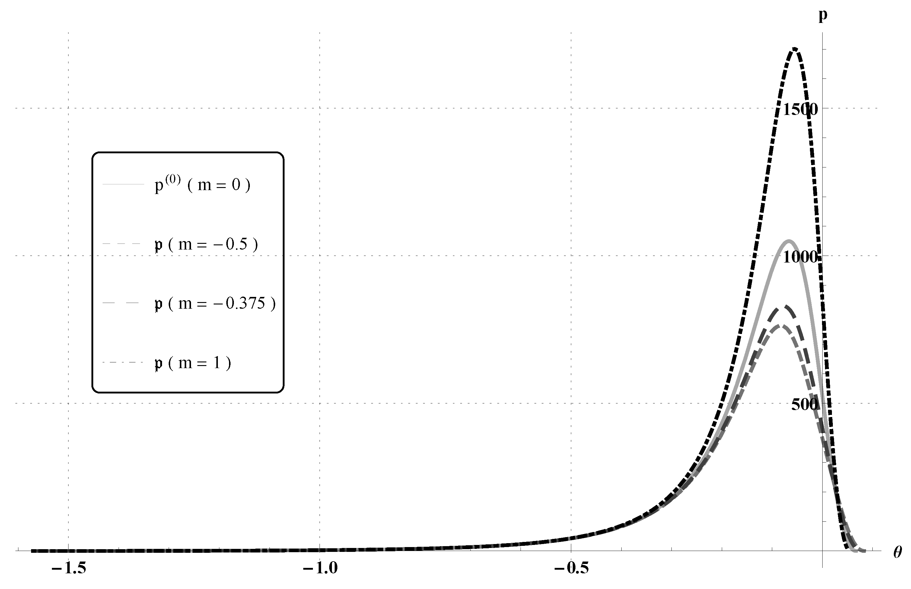
In Figure 2, we plot $\mathfrak{p}$ for $ϵ=0.1$, considering the power-law exponent values $m=-0.5,-0.375,1$, and compare the pressure profiles with $p^{\left(0\right)}$.

For $ϵ=0.1$, the value of the cavitation angle in the classical case ($m=0$) is ${\theta }_1=0.197408$ and the normal force is ${\omega }_{\mathfrak{p}}^{\prime }={\int }_{-\frac{\pi }{2}}^{{\theta }_1}cos\theta p^{\left(0\right)}(\theta )\mathrm{d}\theta =13.985$ in non-dimensional units. In

Table 1. Cavitation angles ${\theta }_2$ and the normal forces ${\omega }_{\mathfrak{p}}^{\prime }$, computed for $m=-0.5,-0.375,1$, when $ϵ=0.1$.

m	${\mathbf{\theta }}_2$ (rad)	${\mathbf{\omega }}_{\mathfrak{p}}^{\prime }$
−0.5	0.245119	10.7558
−0.375	0.229178	11.5351
1	0.167257	20.8097

, we present the values of the cavitation angle ${\theta }_2$ and the corresponding normal forces for the power-law lubrication approximations.

In Figure 3 and

Table 2. Cavitation angles ${\theta }_2$ and the normal forces ${\omega }_{\mathfrak{p}}^{\prime }$, computed for $m=-0.5,-0.375,1$, when $ϵ=0.01$.

m	${\mathbf{\theta }}_2$ (rad)	${\mathbf{\omega }}_{\mathfrak{p}}^{\prime }$
−0.5	0.0827747	181.54
−0.375	0.077616	191.168
1	0.0553576	306.272

, we document the same results when $ϵ=0.01$. The classical ($m=0$) cavitation angle is now ${\theta }_1=0.0666263$ (radians) and the normal force ${\omega }_{\mathfrak{p}}^{\prime }=221.456$.

3.1.2. ${\alpha }_0=\mathcal{O}\left({ϵ}^2\right)$

In this case, we need to solve (numerically) the following nonlinear system for $p^{\left(0\right)}$ and $u^{\left(1\right)}$:

$$\begin{array}{cc}\hfill {\displaystyle \frac{\mathrm{d}{p}^{\left(0\right)}}{\mathrm{d}\theta }}& =cos\theta {\left(1+\frac{\alpha }{2}{\left(\frac{\partial u^{\left(1\right)}}{\partial y}\right)}^2\right)}^{m-1}\left[\frac{{\partial }^2{u}^{\left(1\right)}}{\partial y^2}+{\displaystyle \frac{\alpha }{2}}(n-1){\left(\frac{\partial u^{\left(1\right)}}{\partial y}\right)}^2\frac{{\partial }^2{u}^{\left(1\right)}}{\partial y^2}\right],\hfill \\ & \frac{\mathrm{d}{p}^{\left(0\right)}}{\mathrm{d}\theta }{\int }_0^{h\left(\theta \right)}y(y-h\left(\theta \right)){\left(1+\frac{\alpha }{2}{\left(\frac{\partial u^{\left(1\right)}}{\partial y}\right)}^2\right)}^{1-m}\mathrm{d}y\hfill \\ & =-cos\theta {\left[h\left(\theta \right)+{\displaystyle \frac{\alpha (n-1)}{6}}{\int }_0^{h\left(\theta \right)}(2y-h\left(\theta \right)){\left(\frac{\partial u^{\left(1\right)}}{\partial y}\right)}^3\mathrm{d}y\right]}_{{\theta }_2}^{\theta }.\hfill \end{array}$$

(70)

The boundary conditions for the pressure are the Swift-Stieber conditions, i.e.,

$$p^{\left(0\right)}\left({\theta }_2\right)=0,\frac{\mathrm{d}{p}^{\left(0\right)}}{\mathrm{d}\theta }\left({\theta }_2\right)=0,$$

(71)

and for the velocity those given in (49) and (50).

The computed pressure distributions have been plotted in Figure 4, for $ϵ=0.1$, and in Figure 5, for $ϵ=0.01$. In each case, we have considered the values of power-law exponent $-0.5,-0.375$ and 1 and compared the distributions with that of the classical Newtonian case ($m=0$). The values of the corresponding cavitation angles and the normal forces are given in

Table 3. Cavitation angles ${\theta }_2$ and the normal forces ${\omega }_{\mathfrak{p}}^{\prime }$, computed for $m=-0.5,-0.375,0,1$ when $ϵ=0.1$.

m	${\mathbf{\theta }}_2$ (rad)	${\mathbf{\omega }}_{\mathfrak{p}}^{\prime }$
−0.5	0.221825	11.105
−0.375	0.225363	11.5739
0	0.197408	13.985
1	0.227645	15.2337

and

Table 4. Cavitation angles ${\theta }_2$ and the normal forces ${\omega }_{\mathfrak{p}}^{\prime }$, computed for $m=-0.5,-0.375,0,1$ when $ϵ=0.01$.

m	${\mathbf{\theta }}_2$ (rad)	${\mathbf{\omega }}_{\mathfrak{p}}^{\prime }$
−0.5	0.0747584	189.875
−0.375	0.0760101	194.649
0	0.0666264	221.456
1	0.0774216	233.142

.

In general, the results are similar to the linear case. However, the maxima for the power-law pressures are now shifted to the left with respect to the classical Newtonian case.

3.2. Journal Bearing

Consider an (infinitely) long journal bearing consisting of a cylinder (journal) rotating eccentrically, at an angular velocity $\Omega$, inside another cylinder (bearing) filled with an incompressible power-law fluid.

We denote the journal radius by $R_0$, the bearing radius by R ($R_0<R$) and the distance between centers by a, see Figure 6. We define $\delta \equiv a/R_0$ and $ϵ\equiv (R-R_0)/R_0$ and assume that the non-dimensional parameters $\delta$ and $ϵ$ are small. The fluid film thickness H can be expressed as a function of the angle $\phi$ measured counter-clockwise from the bearing radius perpendicular to the journal. Measured along the bearing radius, the film thickness is, up to an error of the order of $O\left({\delta }^3\right)$ (see [2]), given by

$$H\left(\phi \right)=R-R_0+acos\left(\phi \right)+{\displaystyle \frac{a^2}{2R_0}}{sin}^2\left(\phi \right).$$

(72)

The non-dimensional film thickness $h\left(\phi \right)$ is defined through $H=R_0ϵh$ and, up to an error of the order of $\mathcal{O}\left({ϵ}^2\right)$, can be written as

$$h\left(\phi \right)=1+\chi cos\left(\phi \right)+ϵ{\displaystyle \frac{{\chi }^2}{2}}{sin}^2\left(\phi \right),$$

(73)

where $\chi =a/(R-R_0)$ is the eccentricity ratio.

The equations we have derived do not take into account the curvature effects. In order to do so, we should express the equations in natural orthogonal coordinates (cf. Nazarov and Videman [22]). Since curvature brings a first-order correction term to the classical Reynolds equations, in geometries such as the journal bearing (see [22]), we will drop the last term in (73) and do not consider the case where the non-Newtonian effects appear at the first-order. The equations for the journal bearing become thus similar to those in Section 3.1, except for the absence of the cosine of the angle and for the angular coordinate being the non-dimensional $x=\phi$. In other words, we make $cos\theta \to 1$ and $\theta \to \phi$ in the equations of Section 3.1. The boundary conditions for the pressure $p^{\left(0\right)}$ are $p^{\left(0\right)}\left(0\right)=p^{\left(0\right)}\left(2\pi \right)$ and $p^{\left(0\right)}\left(\pi \right)=0$. Moreover, we choose $U^0=0$ and $U^h=1$ (the velocity scale is $U=2\pi \Omega R_0$).

3.2.1. ${\alpha }_0=\mathcal{O}\left({ϵ}^3\right)$

We do not consider this case since, as explained above, the curvature effects are of the same order as the first order correction $p^{\left(1\right)}\left(\phi \right)$.

3.2.2. ${\alpha }_0=\mathcal{O}\left({ϵ}^2\right)$

The following pressure profiles were computed choosing (a) $\chi =0.1$, (b) $\chi =0.5$, (c) $\chi =0.95$, see Figure 7, Figure 8 and Figure 9, respectively.

We find that the increase of $\chi$, namely from $\chi =0.1$ to $\chi =0.95$, results in a change in the pressure profile, regardless of the value of n. The maxima are higher for larger values of m, as in the previous example. No change is visible to the zeros of the pressure profile and no change of phase is obtained with regard to changes in n, $\chi$, or $ϵ$.

4. Conclusions

We have given a rigorous derivation of Reynolds type lubrication approximations for a family of non-Newtonian power-law models. Based on a formal perturbation analysis, we have shown that, in the cases considered, lubricating film flows for fluids with shear-dependent viscosities can be approximated by simplified dimensionally reduced models. We have corroborated our theoretical results by presenting numerical computations which show that the pressure profiles behave as expected for shear-thinning fluids.

References

1. Reynolds, O. On the theory of lubrication and its application to Mr Tower’s experiments. Philos. Trans. R. Soc. Lond. 1886, 177, 159–209. [Google Scholar]
2. Szeri, A.Z. Fluid Film Lubrication, 2nd ed.; Cambridge University Press: Cambridge, MA, USA, 2010. [Google Scholar]
3. Bair, S.; Khonsari, M.M. Reynolds equations for common generalized Newtonian models and an approximate Reynolds–Carreau equation. Proc. Inst. Mech. Eng. Part J J. Eng. 2006, 220, 365–374. [Google Scholar] [CrossRef]
4. Myers, T.G. Application of non-Newtonian models to thin film flow. Phys. Rev. E 2005, 72, 066302. [Google Scholar] [CrossRef] [PubMed]
5. Yang, Q.; Huang, P.; Fang, Y. A novel Reynolds equation of non-Newtonian fluid for lubrication simulation. Tribol. Int. 2016, 94, 458–463. [Google Scholar] [CrossRef]
6. Shukla, J.B.; Prasad, K.R.; Chandra, P. Effects of consistency variation of power law lubricants in squeeze film. Wear 1982, 76, 299–319. [Google Scholar] [CrossRef]
7. Park, O.O.; Kwon, M.H. Study on the lubrication approximation of power law fluid. Korean J. Chem. Eng. 1989, 6, 150–153. [Google Scholar] [CrossRef]
8. Johnson, M.W., Jr.; Mangkoesoebroto, S. Analysis of lubrication theory for the power law fluid. J. Tribol. 1993, 115, 71–77. [Google Scholar] [CrossRef]
9. Bourgin, P. Fluid-Film Flows of Differential Fluids of Complexity n Dimensional Approach—Applications to Lubrication Theory. ASME J. Lubr. Technol. 1979, 101, 140–144. [Google Scholar] [CrossRef]
10. Kacou, A.; Rajagopal, K.R.; Szeri, A.Z. A thermodynamic analysis of journal bearings lubricated by non-Newtonian fluids. J. Tribol. 1998, 110, 414–428. [Google Scholar] [CrossRef]
11. Harnoy, A. Three dimensional analysis of the elastico-viscous lubrication in short journal bearings. Rheol. Acta 1977, 16, 51–60. [Google Scholar] [CrossRef]
12. Ballal, B.Y.; Rivlin, R.S. Flow of a Newtonian fluid between eccentric rotating cylinders: Inertial effects. Arch. Ration. Mech. Anal. 1976, 62, 237–294. [Google Scholar] [CrossRef]
13. Andres, A.S.; Szeri, A.Z. Flow between Eccentric Rotating Cylinders. J. Appl. Mech. 1984, 51, 869–878. [Google Scholar] [CrossRef]
14. Cal, F.S.; Dias, G.A.S.; Pereira, B.M.M.; Pires, G.E.; Rajagopal, K.R.; Videman, J.H. On the lubrication approximation for a class of viscoelastic fluids. Int. J. Nonlinear Mech. 2016, 87, 30–37. [Google Scholar] [CrossRef]
15. Barus, C. Isothermals, isopiestics and isometrics relative to viscosity. Am. J. Sci. 1893, 45, 87–96. [Google Scholar] [CrossRef]
16. Bair, S. High Pressure Rheology for Quantitative Elastohydrodynamics; Elsevier: Amsterdam, The Netherlands, 2007. [Google Scholar]
17. Rajagopal, K.R.; Szeri, A. On an inconsistency in the derivation of the equations of elastohydrodynamic lubrication. Proc. R. Soc. Lond. A Math. Phys. Sci. 2003, 459, 2771–2786. [Google Scholar] [CrossRef]
18. Gustafsson, T.; Rajagopal, K.R.; Stenberg, R.; Videman, J. Nonlinear Reynolds equation for hydrodynamic lubrication. Appl. Math. Model. 2015, 39, 5299–5309. [Google Scholar] [CrossRef]
19. Fusi, L.; Farina, A.; Rosso, F.; Roscani, S. Pressure driven lubrication flow of a Bingham fluid in a channel: A novel approach. J. Non-Newton. Fluid Mech. 2015, 221, 66–75. [Google Scholar] [CrossRef]
20. Rajagopal, K.R. Implicit constitutive relations for fluids. J. Fluid Mech. 2006, 550, 243–249. [Google Scholar] [CrossRef]
21. Rajagopal, K.R.; Srinivasa, A.R. A Gibbs-potential-based formulation for obtaining the response functions for a class of viscoelastic materials. Proc. R. Soc. Lond. A Math. Phys. Sci. 2011, 467, 39–58. [Google Scholar] [CrossRef]
22. Nazarov, S.A.; Videman, J.H. A modified nonlinear Reynolds equation for thin viscous flows in lubrication. Asymptot. Anal. 2007, 52, 1–36. [Google Scholar]
23. Rajagopal, K.R. Remarks on the notion of “pressure”. Int. J. Nonlinear Mech. 2015, 71, 165–172. [Google Scholar] [CrossRef]
24. Málek, J. Mathematical properties of flows of incompressible power-law-like fluids that are described by implicit constitutive relations. Electron. Trans. Numer. Anal. 2008, 31, 110–125. [Google Scholar]
25. Málek, J.; Rajagopal, K.R.; Ruzicka, M. Existence and regularity of solutions and stability of the rest state for fluids with shear dependent viscosity. Math. Model. Methods Appl. Sci. 1995, 6, 789–812. [Google Scholar] [CrossRef]
Figure 1. Cross-sectional geometry of an infinite cylinder rolling counter-clockwise on a plane. The fluid is between the cylinder and the flat surface. Reprinted from [14], with permission from Elsevier.
Fluids 04 00098 g001
Figure 2. Pressure distributions computed from the classical Reynolds equation, p ( 0 ) ( θ ) ( m = 0 ) , and from the power-law system of Reynolds type equations, p ( θ ) ( m = 0.5 , 0.375 , 1 ) , with ϵ = 0.1 and α 0 = O ( ϵ 3 ) .
Fluids 04 00098 g002
Figure 3. Pressure distributions computed from the classical Reynolds equation, p ( 0 ) ( θ ) ( m = 0 ) , and from the power-law system of Reynolds type equations, p ( θ ) ( m = 0.5 , 0.375 , 1 ) , with ϵ = 0.01 and α 0 = O ( ϵ 3 ) .
Fluids 04 00098 g003
Figure 4. Pressure distributions computed from the classical Reynolds equation, p ( 0 ) ( θ ) ( m = 0 ) , and from the power-law system of Reynolds type equations, p ( 0 ) ( θ ) ( m = 0 . 5 , 0 . 375 , 1 ) , with ϵ = 0.1 and α 0 = O ( ϵ 2 ) .
Fluids 04 00098 g004
Figure 5. Pressure distributions computed from the classical Reynolds equation, p ( 0 ) ( θ ) ( m = 0 ) , and from the power-law system of Reynolds type equations, p ( 0 ) ( θ ) ( m = 0 . 5 , 0 . 375 , 1 ) , with ϵ = 0.01 and α 0 = O ( ϵ 2 ) .
Fluids 04 00098 g005
Figure 6. Cross-section of an infinite journal bearing. The journal is centered at O J and rotates counter-clockwise within the fixed bearing centered at O B . The fluid occupies the space between the two cylinders. Reprinted from [14], with permission from Elsevier.
Fluids 04 00098 g006
Figure 7. Pressure distributions computed from the classical Reynolds equation, p ( 0 ) ( θ ) ( m = 0 ) , and from the power-law system of Reynolds type equations, p ( 0 ) ( θ ) ( m = 0 . 375 , 0 . 25 , 1 ) , with χ = 0.1 .
Fluids 04 00098 g007
Figure 8. Pressure distributions computed from the classical Reynolds equation, p ( 0 ) ( θ ) ( m = 0 ) , and from the power-law system of Reynolds type equations, p ( 0 ) ( θ ) ( m = 0 . 375 , 0 . 25 , 1 ) , with χ = 0.5 .
Fluids 04 00098 g008
Figure 9. Pressure distributions computed from the classical Reynolds equation, p ( 0 ) ( θ ) ( m = 0 ) , and from the power-law system of Reynolds type equations, p ( 0 ) ( θ ) ( m = 0 . 375 , 0 . 25 , 1 ) , with χ = 0.95 .
Fluids 04 00098 g009