Abstract
Direct modeling of time-dependent transport and reactions in realistic heterogeneous systems, in a manner that considers the evolution of the quantities of interest in both, the macro-scale (suspending fluid) and the micro-scale (suspended particles), is currently well beyond the capabilities of modern supercomputing. This is understandable, since even a simple system such as this can easily contain over 107 particles, whose length and time scales differ from those of the macro-scale by several orders of magnitude. While much can be gained by applying direct numerical solution to representative model systems, the direct approach is impractical when the performance of large, realistic systems is to be modeled. In this study we derive and analyze a “hybrid” model that is suitable for fibrous reactors. The model considers convection/diffusion in the bulk liquid, as well as intra-fiber diffusion and reaction. The essence of our approach is that diffusion and (first-order) reaction in the intra-fiber space are handled semi-analytically, based on well-established theory. As a result, the problem of intra-fiber transport and reaction is reduced to an easily solvable set of ODEs, where is the number of terms in the Bessel expansion evaluated without recourse to approximation; this set is coupled, point-wise, with a numerical model of the macro-scale. When the latter is discretized using N nodes, the total “hybrid” model for the system consists of a system of ODEs, which is easily solvable on a modest workstation. Parametric analyses are presented and discussed.
1. Introduction
The modeling of coupled flow and transport/reaction in systems comprised of a solid phase dispersed in a fluid phase has long been of interest to scientists and engineers. These systems involve heat/mass transfer processes occurring at multiple time/length scales [1,2,3] and are found in a wide range practical applications. Examples range from bioreactors [4] to catalytic cracking [5], where the solid phase may be mobile, as in fluidized bed reactors, or fixed in place. Other areas of application are found in the food industry, in the form of drying [6] and meat processing [7]. The particles themselves can be porous, so a complete model must take into account transport in the carrier fluid, as well as the exchange with and diffusion/reaction within the particles.
A single complete analytical solution is not possible for such systems, so many different approaches have been used in their simplification and solution. The problem can be simplified by focusing on the steady state solution and, in some cases, ignoring the diffusion within the particles [8]. However, even these assumptions still lead to a demanding numerical problem. In addition, transient solutions are desirable as they allow more information to be extracted, especially when model predictions are compared with dynamic experiments [6]. Another approach is to focus on only a single spatial scale, modeling diffusion in a single structure [7]. Internal diffusion has also been taken into account in countercurrent plug flow problems by relating the average concentration within the particles to the local concentration in the fluid [9].
In the past few decades, advances in multi-scale and homogenization theories [10], as well as in Computational Fluid Dynamics (CFD) codes and computing facilities, have pushed the boundaries of what can be solved numerically [11]. Particle Resolved Simulations can solve the local heat/mass transfer equations at the particle scale for both fixed and fluidized beds [12]. Detailed particle-based approaches have been proposed using the simulation of a small number of particles in repeating unit cells [3]. One drawback of directly solving the microscale transport equations in every single particle is that prohibitively large meshes are required for, macroscopically, large systems. The problem is more acute in time-dependent simulations, and poses a severe restriction in simulating real-life situations, in which micron- or sub-micron-sized particles may be used.
The purpose of this work is to derive and present a hybrid (semi-analytical) solution to the problem of coupled micro/macro scale mass-transfer in reactors containing fibers (micro-scale) oriented transversely to the bulk flow. Besides intra-fiber diffusion, we also consider a first-order reaction to be taking place within the fibers. This work utilizes the approach previously used for reactors containing spherical catalyst particles and extends it to fibrous systems [13]. The key assumption in the solution derivation is that individual fibers are treated as if they are surrounded by a liquid of a uniform albeit time-varying concentration. Besides a small fiber diameter, this assumption is more likely to hold when the bulk flow is transverse to the fiber axis, implying that our systems also consist of unidirectional fibers. The concentration in the liquid phase (macro-scale) is resolved using the well-established dispersion model. The proposed model only requires meshing of the macro-scale, while the intra-particle concentration is described by a semi-analytical formula which requires the solution of a small number of ODEs. This is easily tractable using standard ODE solvers.
Although this specific study is using the axial dispersion model to describe the transport in the bulk liquid, the fiber-scale model is portable to any other macroscopic situation, as long as the fibers are small relative to the concentration gradients in the bulk liquid. In Section 2, the development of the model will be outlined for the case of constant reactor porosity, fiber porosity, and radius; this is not a necessary assumption and the model can be modified to accept spatially varying parameters.
2. Model Development
The general approach of the outlined semi-analytical solution is to use the local surface concentration () in the fiber phase as a time-varying boundary condition for the intra-fiber transport problem. The analytical solution for the concentration profile in the fiber is approximated by expanding the solution in Bessel functions. The concentration profile allows for the calculation of the flux from the liquid phase to the fiber phase, yielding an equation for the local liquid concentration (). Discretization of the bulk scale leads to a system of ODEs which can be easily solved using standard numerical methods.
2.1. Problem Description
In order to describe the dynamic response of the system shown in Figure 1, the governing differential equations for the mass transfer in the bulk liquid and the mass transfer/consumption in the intra-fiber space must be solved. The boundary condition at the surface of the fiber governs the mass transfer between the fibers and the bulk liquid, therefore providing the link between the micro (intrafiber spaces) and macro (bulk liquid) scales of the problem. The axial distance along the reactor and the radial co-ordinate in a fiber are the two spatial independent variables, while the time is the third independent variable. In a manner similar to earlier studies [13,14] the following phenomena are taken into account in the following analysis:
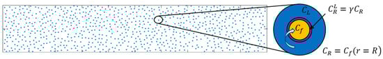
Figure 1.
Schematic of the system. The species can be transported from the bulk liquid across the boundary layer and into the fiber, where it can diffuse and react within the fiber’s pores.
- Mass accumulation in the bulk liquid.
- Mass diffusion from the bulk liquid, across the boundary layer, and into the fibers.
- Mass diffusion, accumulation and consumption (via a first-order chemical reaction) in the intra-fiber space.
- Axial dispersion in the bulk liquid.
The operating assumptions of the model are:
- The fiber locations are fixed.
- The system is isothermal.
- The first order reaction constant and the intra-fiber diffusion coefficient are constant.
- The bulk liquid concentration gradients in the perpendicular plane (along the fiber length), fiber aging and the pressure drop in the reactor are negligible. This implies that the bulk flow is strictly transverse to the fiber axes.
- The fibers are of uniform size and uniformly dispersed along the reactor.
2.2. Model Development
The following equation describes the mass transfer, accumulation, and consumption in the intra-fiber space:
where is the concentration in the intra-fiber pore volume, is the effective intrafiber diffusivity, is the first order reaction rate constant, and is the fiber void fraction. The initial and boundary conditions are given by
where is the concentration in the bulk liquid, is the liquid concentration at the inner side of the boundary layer around the fiber, and is the external mass transfer coefficient. is related to the fiber surface concentration () via a partition coefficient, . The bulk-fluid concentration CL Equation (4) links the micro- and the macro-scale processes. This microscale flux across the fiber surface Equation (4) can be multiplied by the total fiber surface area per unit volume of reactor to yield the flux from the bulk liquid to the fibers at any axial position in the reactor, .
where is the reactor void fraction, is the fiber radius, is the bulk flow rate, and the total reactor volume.
Using the dispersion model, in dimensionless form, the mass balance in the bulk liquid is
in which, is the Péclet number, describing the relative strength of convection and diffusion in the bulk liquid, is the dimensionless axial position, and is the dimensionless time. Evidently, the flux term () in Equation (5) links the micro Equation (1) and macro Equation (6) scales of the problem. The three terms on the right-hand side of Equation (6) are the mass flux due to diffusion, convection, and transfer to the fibers. The initial and boundary conditions are
As explained in Appendix A, the analytical solution of Equation (1) (available at constant surface concentration) is used to derive an expression for the intra-fiber concentration, subject to a time-varying surface concentration. The result is that the fiber surface concentration () can be determined by solving the following ODE:
The terms appearing in Equation (11) are described by ODEs of the form.
As a result, and as explained in the Appendix A, the fluid-to-fiber mass flux can be evaluated either via the difference between the surface and liquid concentration Equation (12) or using the summation of the terms Equation (13).
In short, the microscale discretization of the fibers has been avoided and, instead, a system of ODEs describe the evolution of , , at a given axial position. Equation (6) can then be discretized in the axial direction and written, in dimensionless form at axial node , as:
The ODEs defined by Equations (10), (11), and (14) are applicable at each node, leading to a system of ODEs, which can be solved using standard ODE solvers such as ode45 or ode113 available in MATLAB.
3. Results
We have performed a series of simulations using MATLAB ODE solvers ode45 or ode113 over a range of dimensionless parameter values. The Thiele Modulus, , describing the ratio of the reaction rate to the diffusion rate inside the fiber, varied from 0 to 100. The Biot number, , describes the ratio of the external to internal mass transfer resistances varied from 10−3 to 100. The dimensionless diffusivity, , was varied from 0.001 to 100. Fiber voidage, and Péclet number, , were also varied.
Model predictions concerning the effect of the Péclet number, in the presence and absence of intra-fiber porosity, are shown in Figure 2. When porous fibers are considered, there is transfer of the reactant from the bulk as the species diffuse into the fibers. This results in a modified effluent profilecompared to the impermeable (solid) fibers case. This effect is more pronounced at high Péclet numbers.
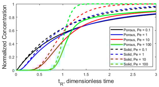
Figure 2.
The effect of the Peclet Number on the effluent concentration profile for solid and porous fibers ().
The effect of the Biot number is shown in Figure 3 for two different levels of diffusivity for a non-reacting species ( = 0). In each case, very low Biot numbers lead to the condition where the liquid concentration profile is limited by a high external mass transfer resistance to the fibers, leading to a negligible amount of exchange between the two phases. On the other end of the spectrum the internal resistance of the fibers dominates. The Biot numbers that correspond to these limiting cases are dependent on the other system parameters, such as . For the intermediary cases, the and terms both play a role as neither internal, nor external mass transfer resistances dominate.
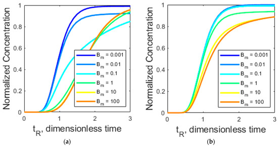
Figure 3.
Normalized concentration profiles as a function of when diffusivity is (a) high, =10 and (b) low ().
In Figure 4, the Thiele modulus is varied from 0 to 100 and the effect on the effluent profile and the radial concentration profile, computed from Equation (A5) within a fiber at the end of the reactor at are shown. When is very low, the reaction is rate-limited as the reactant is consumed very slowly and builds up in the fiber. When is very large the reaction in the fibers proceeds very quickly and the mass flux to the fiber is not large enough to sustain a high concentration in the fiber; this corresponds to the mass transfer limited regime. In between the two extremes, all the parameters play their role in the process.
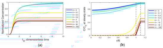
Figure 4.
(a) Effluent profile and (b) intra-fiber concentration profile at the end of the reactor and ).
4. Case Study
A hybrid, semi-analytical model for coupled flow and mass-transfer processes in reactors containing fibers oriented perpendicular to the direction of bulk flow has been presented in Section 2, with some results of parametric analyses being shown in Section 3. This model is also applicable to situations where the fiber radii/porosities vary along the reactor. This is because the relationship we derive between the surface concentration in the fiber and that of the bulk liquid apply at each axial position. The appropriate constants from Equations (11)–(13) would simply need to be replaced by their values at node . Another example would be the case where the reactor voidage is not constant along the reactor, representing bundles of fibers placed at different locations. Such a case is shown in Figure 5, in which a decreased voidage over 10 percent of the reactor length is introduced at three positions: near the inlet, at the center, and near the outlet. The constant voidage example having the same average over the reactor is also shown.
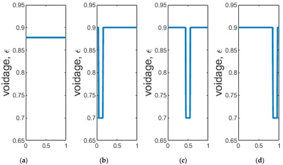
Figure 5.
Reactor voidage () vs axial position for four different profiles having the same total reactor voidage (a) constant profile, and decreased voidage (b) near the linlet (c) at the center (d) near the outlet.
The results of the analysis of the cases represented in Figure 5, in terms of effluent concentrations and axial concentration profiles at steady state, are shown in Figure 6. With all other factors remaining constant, the location of the fiber bundle does appear to slightly affect the transient response of the system (Figure 6a), the fiber bundles leading to a slightly increased conversion of the feed material within the reactor. This example illustrates one of the advantages of the semi-analytical model, as it can easily capture differences that would have been ignored by the simplifications used in a model based on bulk/effective properties.
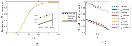
Figure 6.
(a) effluent concentrations for the various voidage profiles shown in Figure 5; (b) the steady state axial concentration profile, dashed lines correspond to liquid concentration and solid lines to the volume-averaged concentration in the intrafiber space ).
Author Contributions
Conceptualization, T.D.P.; Formal analysis, A.D.; Funding acquisition, T.D.P.; Investigation, A.D.; Methodology, T.D.P. & A.D.; Writing—original draft, A.D.; Writing—review & editing, T.D.P. All authors have read and agreed to the published version of the manuscript.
Funding
This work was carried out with support from Grant Award Number 090118FD5313 under the “Structure-Property Correlations in Multi-Scale Composites” project at Nazarbayev University.
Conflicts of Interest
The authors declare no conflict of interest.
Notation of Parameters
| positive roots of , where is a Bessel function of order | |
| reactor void fraction | |
| intra-fiber void fraction | |
| partition coefficient, | |
| functions defined by Equations (6) and (7) | |
| integration variable used in application of Duhamel’s Theorem | |
| Thiele modulus, | |
| Biot number (dimensionless), | |
| concentration in the bulk liquid at the inlet, mol/L | |
| concentration in the intra-fiber pore volume, mol/L | |
| concentration in the bulk liquid, mol/L | |
| concentration at the fiber surface, mol/L | |
| concentration at the innter side of the boundary layer, mol/L | |
| effective intrafiber diffusivity, m²/s | |
| axial dispersion coefficient, m²/s | |
| dimensionless diffusivity, | |
| reactor flow rate, L/s | |
| the parameter in parentheses evaluated at node | |
| first order reaction rate constant, s−1 | |
| external mass transfer coefficient, m/s | |
| parameter defined in Appendix A as | |
| reactor length, m | |
| number of terms to be solved | |
| number of nodes in the spatial discretization | |
| Péclet number, | |
| r | radial position within the fiber, m |
| fiber radius, m | |
| summation defined by Equation (A13) | |
| time, s | |
| dimensionless time, | |
| axial fluid velocity in the reactor, m/s | |
| total reactor volume, L | |
| dimensionless axial distance, | |
| axial distance from inlet, m |
Appendix A
Intra-Fiber Concentration Profile in the Presence of Diffusion and 1st Order Reaction under a Time-Varying Surface Concentration
The first step in the solution to Equation (1) subject to a time-varying surface concentration relies on existing analytical solution for diffusion inside a cylinder [8,9] initially at zero concentration and subject to a constant surface concentration of for . This solution is:
is the Bessel function of order , are the positive roots of and . When a first-order reaction is present Danckwert’s method [15] can be used to show that the time-dependent concentration profile in the fiber (C2) for the same constant surface concentration is given by
Using Equation (A1) to evaluate Equation (A2) leads to the following intra-fiber concentration profile for constant surface concentration and in the presence of diffusion and first-order reaction
The normalized concentration profile under a time-varying surface concentration () can now be found using Duhamel’s Theorem [8]
Carrying out the integrations, the resulting expression for the intra-fiber profile, under a time-varying surface concentration, , is given by
where the functions are given by
or in differential form by
with initial conditions . The derivative in Equation (5) can now be evaluated, using Equation (A5), as
The relationship between the surface concentration and liquid concentration can therefore be written as
And the flux term can be calculated either via the difference between the surface and the liquid concentration Equation (A10) or via the summation of the terms Equation (A11).
The large/increasing values of the factor multiplying the term ( are monotonously increasing) in Equation (A7) imply that, at large , the functions follow the forcing function on the right hand side of the equation. Above a certain threshold, the terms can be approximated using the quasi-steady state approximation
The infinite summation in Equation (A9) is therefore split into two parts, with the first terms being evaluated using Equation (A7) and the rest of the summation to infinity being approximated by Equation (A12).
Examples of the time-varying terms of different orders and their steady state approximations using Equation (A12) (dashed lines, denoted “S.S.”) are shown in Figure A1a,b. The lower order n terms (Figure A1a) are poorly approximated by Equation (A12) and clearly outweigh the higher order terms, which can be reasonably approximated by Equation (A12) (Figure A1b). Computing more than the first ≈ 50 terms does not noticeably impact the result of the summation for the example under consideration in Figure A1c. In general, more terms will be necessary for a good approximation when the term is large.

Figure A1.
Examples of the form and relative magnitude of terms and their steady state approximations for (a) n = 1–5 (b) n = 5, 10, 15, 20, 25, 30 and 25 (c) the result of summation for ranging from 2 to 200. With N = 50, this corresponds to a system of between 200 and 10,100 ODEs (in all cases shown, Pe = 10, ).

The relationship between the accuracy and is more clearly shown in Figure A2a where the maximum error (over the timescale shown in Figure A1) relative to the case of = 200 is shown for two different variables; namely, and . The number of terms to be calculated to reach a desired level of accuracy for a given reactor can further depend on the variable of interest, for example the effluent concentration requires fewer terms than the concentration at the fiber center to reach a certain accuracy threshold. As increases, the computation time also increases significantly, as shown in Figure A2b, therefore the should be selected to balance accuracy and computation time for each reactor. A model based on a similar method of solution of the multi-scale problem has been used in [16] for the prediction of the response of a fixed bed made of Ca-Alginate gel particles. It was found that model predictions were in excellent agreement to experimental results, which exhibited the same, qualitatively distinct, features predicted by the model.

Figure A2.
(a) Error in concentration, relative to the case vs (b) MATLAB solver runtime (on a HP Z4 workstation) vs .
Figure A2.
(a) Error in concentration, relative to the case vs (b) MATLAB solver runtime (on a HP Z4 workstation) vs .

Equations (A9) and (A13) combine to yield the differential equation for the surface concentration as a function of the bulk liquid concentration and the process parameters.
where is the summation
References
- Cardellini, A.; Fasano, M.; Bigdeli, M.B.; Chiavazzo, E.; Asinari, P. Thermal transport phenomena in nanoparticle suspensions. J. Phys. Condens. Matter 2016, 28. [Google Scholar] [CrossRef] [PubMed]
- Gooneie, A.; Schuschnigg, S.; Holzer, C. A review of multiscale computational methods in polymeric materials. Polymers 2017, 9. [Google Scholar] [CrossRef] [PubMed]
- Sengar, A.; Kuipers, J.A.M.; van Santen, R.A.; Padding, J.T. Towards a particle based approach for multiscale modeling of heterogeneous catalytic reactors. Chem. Eng. Sci. 2019, 198, 184–197. [Google Scholar] [CrossRef]
- Boyle-Gotla, A.; Jensen, P.D.; Yap, S.D.; Pidou, M.; Wang, Y.; Batstone, D.J. Dynamic multidimensional modelling of submerged membrane bioreactor fouling. J. Membr. Sci. 2014, 467, 153–161. [Google Scholar] [CrossRef]
- Fusheng, O.; Yongqian, W.; Qiao, L. A lumped kinetic model for heavy oil catalytic cracking FDFCC process. Pet. Sci. Technol. 2016, 34, 335–342. [Google Scholar] [CrossRef]
- da Silva, W.P.; Precker, J.W.; Silva, C.M.D.P.S.E.; Gomes, J.P. Determination of effective diffusivity and convective mass transfer coefficient for cylindrical solids via analytical solution and inverse method: Application to the drying of rough rice. J. Food Eng. 2010, 98, 302–308. [Google Scholar] [CrossRef]
- Graiver, N.; Pinotti, A.; Califano, A.; Zaritzky, N. Mathematical modeling of the uptake of curing salts in pork meat. J. Food Eng. 2009, 95, 533–540. [Google Scholar] [CrossRef]
- Olafadehan, O.A.; Aribike, D.S.; Adeyemo, A.M. Mathematical modeling and simulation of steady state plug flow for lactose-lactase hydrolysis in fixed bed. Theor. Found. Chem. Eng. 2009, 43, 58–69. [Google Scholar] [CrossRef]
- Kerkhof, P.J.A.M. Countercurrent plug flow mass exchange with internal particle diffusion. Chem. Eng. Sci. 2007, 62, 2040–2067. [Google Scholar] [CrossRef]
- Andrievsky, A.; Brandenburg, A.; Noullez, A.; Zheligovsky, V. Negative magnetic eddy diffusivities from the test-field method and multiscale stability theory. Astrophys. J. 2015, 811. [Google Scholar] [CrossRef]
- Bec, J.; Biferale, L.; Cencini, M.; Lanotte, A.; Musachio, S.; Toschi, F. Heavy particle concentration in turbulence at dissipative and inertial scales. Phys. Rev. Lett. 2007, 98. [Google Scholar] [CrossRef] [PubMed]
- Sulaiman, M.; Hammouti, A.; Climent, E.; Wachs, A. Coupling the fictitious domain and sharp interface methods for the simulation of convective mass transfer around reactive particles: Towards a reactive Sherwood number correlation for dilute systems. Chem. Eng. Sci. 2019, 198, 334–351. [Google Scholar] [CrossRef]
- Papathanasiou, T.D.; Kalogerakis, N.; Behie, L.A. Dynamic modelling of mass transfer phenomena with chemical reaction in immobilized-enzyme bioreactors. Chem. Eng. Sci. 1988, 43, 1489–1498. [Google Scholar] [CrossRef]
- Papadakis, E.; Pedersen, S.; Tula, A.K.; Fedorova, M.; Woodley, J.M.; Gani, R. Model-based design and analysis of glucose isomerization process operation. Comput. Chem. Eng. 2017, 98, 128–142. [Google Scholar] [CrossRef]
- Crank, J. The Mathematics of Diffusion, 2nd ed.; Oxforn University Press: London, UK, 1975. [Google Scholar]
- Papathanasiou, T.D.; Bijeljic, B. Intraparticle diffusion alters the dynamic response of immobilized cell/enzyme columns. Bioprocess Eng. 1998, 18, 419–426. [Google Scholar] [CrossRef]


© 2019 by the authors. Licensee MDPI, Basel, Switzerland. This article is an open access article distributed under the terms and conditions of the Creative Commons Attribution (CC BY) license (http://creativecommons.org/licenses/by/4.0/).