Abstract
The paper presents the theoretical basis for the extension of the VLES method, originally developed in recent works of the authors for incompressible flows, to flows with variable density and transport properties but without chemical reactions. The method is based on the combination of grid based and grid free computational particle techniques. Large scale motions are modelled on the grid whereas the fine scale ones are modelled by particles. The particles represent the fine scale vorticity, and scalar quantities like e.g., temperature, mass fractions of species, density and mixture fraction. Coupled system of equations is derived for large and fine scales transport.
1. Introduction
In our previous works [1,2,3] we propose a novel numerical technique, referred to as the VLES approach, which utilizes the combination of grid based and grid free computational methods. The large scale motions are modeled on the grid whereas the fine scales are represented by vortex particles. Advantages of the new technique were clearly demonstrated in validation tests for canonical wall free flows. At present, the validation is continued for wall bounded flows, which results will soon be published. The idea of the method is relatively simple. Due to inherent instability of turbulent flows, the grid based solution shows the tendency to create flow structures with sizes comparable with the cell size. In grid based methods, these structures either disappear due to artificial viscosity in schemes with a low order accuracy or result in a high frequency instability which is well seen in the spectra as a pile up of the kinetic energy at high frequencies [2] when high order schemes are utilized. Within the framework of VLES such structures are recognized and converted to vortex particles which don’t depend on the grid. A fundamental assumption of the VLES approach is the decomposition of any physical quantity, say the velocity , into the grid based (large scale) and the fine scale parts, whereas is resolved on the grid and is represented by particles. Dynamics of large and fine scales is calculated from two coupled transport equations one of which is solved on the grid whereas the second one utilizes the Lagrangian grid free Vortex Particle Method (VPM). We classified the method as the Large Eddy Simulation (LES) with a direct resolution of the subgrid (SG) motion modeled by part. Numerical simulations [2,3] showed that vortex particles play a role as triggers or intensifiers of the turbulence in the grid based solution. Their inner interaction does not contribute sufficiently to the flow evolution. Hence the name of the method is the LES intensified by the vortex particles or VLES.
The aim of the present paper is to develop a theoretical framework for extension of the VLES method towards flows with variable density and transport properties. Variation of density and transport properties is assumed to be due to change of the temperature and chemical composition of the gas mixture. In this paper, such flows will further be referred to as the compressible flows at low Mach number or just compressible flows. The flow with a constant density is called incompressible in this paper. As the most general case with chemical reactions (e.g., combustion) would rise further questions and increase the volume of this work excessively, the present paper focuses on flows for which mixing and temperature gradients are important, but chemical reactions do not occur. Examples are the distribution of hazardous emissions from chimneys or vehicles in urban environments, flows in air-conditioned rooms and in large atria, exhaust gas recirculation or heat utilization.
Within the framework of VLES (both compressible and incompressible) only the fine scales of vorticity field are represented by particles. The separation between the large and fine scales is done using the spatial LES filtration. Similarly to the incompressible case the fine scale velocity field is calculated from the grid one using the LES filtration operation denoted by overlines:
According to the Helmholtz decomposition every velocity field including the velocity pulsation can be represented as the sum of three components:
The first term is the velocity induced by vorticity, the second one is due to the flow expansion and the third one is the potential velocity arising due to influence of flow boundaries. We suppose that the fine vortices are generated at a some distance far from the boundaries and don’t influence the boundary conditions on boundaries. In this case the boundary effect is entirely taken into account by the large scale velocity , i.e., . As follows from (2) the fine scale velocity should be represented not only by vorticity, but also by expansion sources. Therefore, in contrast to the incompressible case we have to introduce two sorts of particles: vortex particles and expansion particles. In principle they are different, because vortex particles arise in areas of high vorticity whereas the expansion particles should correspond to the areas of high expansion rate characterized by the material derivatives of the density. Although in the paper [4] the same set of particles is used for vortex particles and expansion particles, in this paper we will consider a more general case introducing different particle sets.
The algorithm for determination of the strengths of the vortex particles inducing (see [2,3]) is based on the identification of vortex structures in the field using the criterium [5] which is directly extendable to compressible flows [6]. At locations of large values we insert new vortex particles with the strength being equal to the local vorticity multiplied with the cell volume, where is the velocity induced by vortex particles already present in the flow. The vortex particles induce the velocity which, in the ideal case, should be equal to . Because of discrete representation of by discrete vortex paticles, in the general case we have: and a special rescaling procedure was introduced to match both velocities ([2,3]).
From the physical point of view arises due to the temporal change of the density fluctuation. Modeling of the expansion velocity is considered in details in Section 5.
Mathematical models of the flow with variable density and viscosity implies the solution of additional transport equations for scalar quantities like like, e.g., temperature and mass fraction of chemical species. Solution of the scalar transport equations within the VLES framework is discussed in Section 8.
2. VLES for Incompressible Flows
The purpose of this section is to shortly present the algorithm of the VLES method for incompressible flows to make it easier to understand for compressible ones. The large scale vortices are reproduced on the grid. At each time step, the fine vortices consist of new generating vortices (filled circles) and “old” ones generated in the past (symbols *) (see Figure 1). The main equation governing the large scale motion reads (see [2]):
which is solved using the OpenFOAM. The motion of fine vortices is governed by the Equations (7) and (8). Once at any time instant, the grid solution step is completed, the evolution of fine vortices is carried out in the following sequence: generation, motion, feedback effect on large scales through the term , mapping to the grid or elimination. Below these processes are considered in more details.
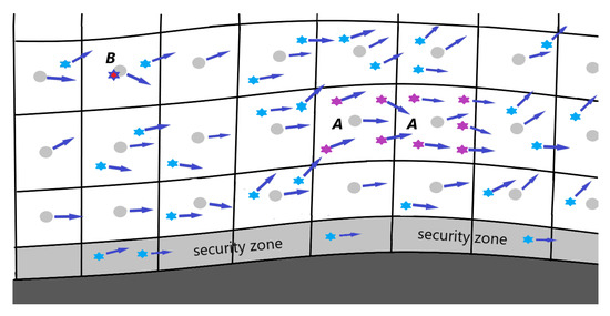
Figure 1.
Vortex particles utilized in VLES method. Filled circles are the vortices newly generated at a time instant at cell centers, * are the fine old vortices generated at previous time steps, the arrows show the velocities of vortices. The security zone is explained in Section 9.
2.1. The Algorithm of Creation of New Vortices
The new generated vortices are responsible for the fine scale velocity field
where is the velocity induced by vortices generated in the previous time steps. The vortex identification criterion [5] is calculated at each cell using the velocity field (4). The cells at which contain the vortex candidates which in principle can be converted to vortex particles. They will be marked as active ones using the field:
where is a certain small value (a free parameter of the algorithm) introduced to sort out the weak vortices. To keep the required computational resources on an acceptable level, only small vortices with size proportional to the local cell size are to be converted to single vortex particles. It is supposed that the larger vortices with scales of a few can accurately be represented on the grid. Therefore, they should be identified and separated from small scale ones. For that, all neighboring cells of the i-th cell are checked for the condition . If all neighbors fulfill this condition we identify a cell cluster which remains on the grid and all their cells become non- active . Such algorithm recognizes A- cells in Figure 2 as those belonging to clusters whereas the cells B are cells with new generating vortices.
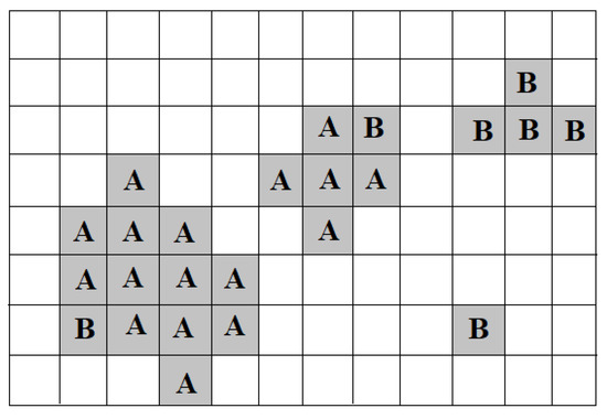
Figure 2.
Cells with (shadowed), cluster cells (A), cells with fine scale vortices converted to vortex particles (B).
Only activated vortices in cells with are to be replaced by vortex particles. At each cell with a single new vortex particle is introduced at the cell center. Thus, each cell contains old vortices and the new one (Figure 1). The radius of the new vortex is set as , where is the overlapping ratio which is taken as and is the volume of the i-th cell. The vortex particle strength is calculated as . If the distance from the new particle to one already existing in the cell is smaller than some permissible distance , they are merged (the cell B in Figure 1).
The velocity , induced by the new generated vortex particles, is calculated at grid points using the Biot-Savart law. The vorticity is not equal to the target vorticity because of discrete particle representation of the continuous vorticity field inducing . Therefore the rescaling procedure should be introduced in the next step of the algorithm:
The rescaled velocity field , induced by the new generated vortex particles, is calculated at grid points using the Bio-Savart law and subtracted from the grid velocity . Thus, the total velocity at grid points remains constant after the vortex particle generation procedure. To keep the number of vortices at any cell restricted, in case of the weakest vortices populating this cell are deleted keeping the total number of vortices per cell less or equal to . At these are cells A in Figure 1. If the number of vortices is less than no vortices are deleted.
2.2. Update Procedure for the Particle Positions and Strengths
The fine vortices (old and new generated ones) are moving and change their strengths. In our previous works [2,3] we showed that the vorticity transport equation can sufficiently be reduced by neglecting inner interaction between vortex particles. With the other words, the motion of vortices and the strength change can be calculated without consideration of the velocity induced by fine vortices. Therefore, in the next step the velocities and tensor are calculated at vortex centers from the OpenFOAM (OF) simulations. The routines for the interpolation of , and from grid points to particles, particle tracking, filtering procedure to calculate were available in OpenFOAM and effectively used to develop a fast working code.
Vortex displacement is found from the equation
The vortex strength is changed according to the algorithm described in Section 6.2, in which the density should be constant, i.e., and the temporal change of the fine vorticity is calculated as
If during the motion the fine vortices become very small due to stretching, they are eliminated.
2.3. Calculation of the Influence of Fine Scales on the Grid Based Solution
The term in (3), which takes the influence of fine scales on the grid based solution, is treated in an explicit way. The velocities are calculated at cell centers using the Biot-Savart law. The grid based vorticity is taken from the OF numerical solution. The filtering is computed using the routines build in the OF code.
2.4. Mapping Big Vortex Particles Back onto the Grid
There is a permanent exchange between the small vortices and large scale ones represented on the grid. Large scale vortices become small due to stretching and are converted to particles according to the algorithm in Section 2.1. If particles grow due to viscosity and flow stagnation and exceed some size they are mapped back to the grid. For that the velocities induced by this vortex particle are calculated at the grid points within adjacent cells and added to the grid based velocities . After that the vortex is deleted from the list of fine vortex particles. can be taken equal to four according to the experience from [3].
3. Momentum and Vorticity Equations for Compressible Flows
Neglecting the volume viscosity, the Navier Stokes equation for compressible flows (see [7], pages 47–53) reads:
where , , p, , are, respectively, density, velocity vector, pressure, body force vector, dynamic viscosity and . Applying curl operator to (9) we get consequently
where
The continuity equation imposes the mass conservation principle, which in case of variable density is:
4. Decomposition of Vorticity and Continuity Equations According to Scales
Following [1], the governing equations of the hybrid grid-free and grid-based method are derived using the decomposition of the velocity, vorticity, density and pressure fields into large scale, represented on the grid, and fine scale, represented by particles, components, i.e.,
Fine scale variations of both kinematic and dynamic viscosity coefficients as well as of diffusion coefficients are neglected as it is common in numerical methods for turbulent flows with mixing, buoyancy or combustion. The same assumption applies also for the pressure fluctuations [8]. Substitution of the decomposition (12) in the (10) gives
The last equation is split in two equations for large and fines scales which are treated in a coupled manner. It should be noted that this splitting is ambiguous (see comments in Section 2 in [2]) and the best choice of it is the matter of experience. In this paper we suggest the following splitting:
The sum of (14) and (15) retrieves the original Equation (13). The first equation is then rewritten in variables to utilize any available CFD code based on a grid method. From (14) we obtain
and
where P is a scalar function referred to as the grid based pressure and
The Equation (16) is solved on the grid whereas the Equation (15) is treated using the VPM. The term takes into account the influence of fine scale motions on large ones. It has the same form as that derived in [1] for incompressible flows. Terms with the upper index “g” in the Equation (15) represent the influence of large scales on small ones.
The continuity equations can be split in a similar way:
The Equations (16) and (17) involve terms of different spatial and time scales. Some terms can become invisible on the grid and need a special treatment. This can lead to the stiffness of these equations which is a common problem in modeling of multiscale physics. An usual way to overcome this problem is the spatial averaging of terms representing fine scales (see [9]) as done in our previous works for incompressible flows [1,2,3]. The spatially filtered equation takes the form:
Solution of the Equation (20) is performed using any grid based method and is further not discussed. Various LES filters build in a grid based code can be used to calculate the spatially averaged terms.
5. Solution of the Continuity Equation
Solution of the Equation (17) can be done in explicit, semi-implicit and fully implicit ways. The presence of the source term on the r.h.s of (17) doesn’t cause principal difficulties. This is true for both explicit time-stepping methods and pressure-correction methods. We first note here, that this term is known at the time when the continuity equation is to be updated on the grid. Both explicit time-stepping and pressure-relaxation methods make use of source-terms, so that the r.h.s. of Equation (20) becomes simply a part of these source terms. Therefore, the computation of Equation (20) does not require any change in conventional algorithms for the solution of the continuity equation.
The remaining question is the handling of the second Equation (18). For that, two strategies are possible. First, one can assume that the whole density is represented only on the grid, i.e., we neglect the subgrid change of the density and the fine scale expansion velocity . For instance, in the recent paper of Ghoniem’s group on combustion [4] only the flow is calculated using the vortex particle method whereas all scalars including the density are computed on the grid. Then only the Equation (17) remains.
Within the second strategy the Equation (18) is taken into account in the computation of the velocity which is calculated from the expansion field (see also the formula (8) in [4]):
where
Introduction of the expansion velocity is a common procedure developed for the application of vortex methods to compressible flows. The expansion velocity is expressed through using the Helmholtz theorem:
Discretization of (22) using the expansion particles is given in [4] (see formulas (15)–(17) on the page 971 in [4]).
The last question to be discussed is the determination of the subgrid density . We consider the case that density is a function of the temperature T and concentration of chemical species Y. Therefore, it is quite reasonable to assume that the particles carrying the fine density fluctuations coincide with those carrying the fine scale fluctuations of the temperature and species which will be introduced in Section 8. In this way we introduce three set of particles. The first one carries the vorticity field, the second one carries the temperature field and the third one describes the transfer of the chemical species. The last two sets carry also the density fluctuations . In case of single-component gases, only the fluctuations of temperature are considered for the density fluctuations. The movement of all particles is calculated from the trajectory equations
where is the particle center. The derivative describes the change of along the particle path:
6. Numerical Solution of the Fine Scale Equation (15) Using VPM
6.1. Relations for Vortex Tubes in Compressible Flows
The algorithm of the solution is based on the Kelvin and Helmholtz theorems which state that for both compressible and incompressible smooth isentropic ideal flows, vortex tubes move with the flow, and their strength remains constant [10]
where is the radius of the vortex tube and is the vorticity in the cross section of the vortex tube. Differentiating (25) on time gives
Conservation of the mass written for the piece of the vortex tube of the length l reads
Derivative of (27) on time provides the formula for the radius change
6.2. Calculation of the Vortex Particle Transport
The formulas derived above are utilized to extend the algorithm [11], which we successfully used in our previous papers [2,3] to calculate the dynamics of vortex particles in incompressible flows, towards compressible flows. In what follows, under the designation is used for the sum . The algorithm consists of the following steps:
- is calculated from the vorticity transport Equation (15) without the viscous diffusion term.
- is calculated from the Equation (24).
- Calculation of the particle length from the equation of the elementary section transported in inviscid flow
- Calculation of the particle core radius from the equation describing the transport of an elementary tube with length l and radius in inviscid flow
- Consideration of the viscosity influence using the core spreading method (CSM) (see [12]). The particle core radius is increased by :
- Calculation of the new particle orientation using the Euler method
- Calculation of the particle strength magnitude from (25)The last equation follows from (25) using the simple algebraic transformations
- Calculation of the new strength vector
In the original version proposed by [11] the next step should be the redistribution of particles whose length is doubled. According to our experience the redistribution results in an avalanche-like increase of the vortex particles number in areas of strong stretching. To prevent this [11] proposed a special elimination procedure based on a knowledge of a threshold for the dissipation rate which is difficult to set in a general flow case. To develop a robust code, to obtain a stable solution and to keep the particle number in a reasonable range we avoid the redistribution procedure in our computations. Thus, the smallest vortices are removed. This reduces the range of scales that must be resolved in a numerical calculation. Such a reduction is an immanent part of every turbulence model.
7. On the Model Reduction
A successful numerical method should provide the desired accuracy and be as simple as possible. At a glance the presented hybrid method may seem not attractive because of its seeming complexity. Especially the equation for the fine vorticity transport Equation (15) seems to be very complicated. However, as shown in [2,3] for the incompressible flow, the vorticity transport equation can sufficiently be reduced by neglecting inner interaction between vortex particles without a significant loss of the simulation accuracy. The following three levels of complexity have been considered for incompressible flows:
- Full vorticity transport equation (full formulation):
- Vorticity transport equation without stretching and convection caused by fine vortices (passive vorton):
- Vorticity transport equation without stretching (designated as the woStrengthUpdating in Figure 3):
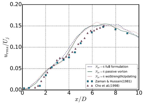
Comparison between three models is presented in Figure 3 for the r.m.s of axial velocity along the axis of the free jet at the Reynolds number of . Detailed description of the jet case and results are presented in [3]. The difference between results obtained using the full model (38), the passive vortices model (39) and the model without stretching term (38) is negligible pointing out that vortex particles serve just as triggers or intensifiers of turbulence and their inner interaction does not contribute sufficiently to the flow evolution. This conclusion raises the quite relevant hypothesis: perhaps the whole theory can radically be simplified, the moving vortex particles can be neglected, the trigger effect can artificially be simulated using any simple and computationally cheap procedure. To prove this hypothesis we left only new generated vortices, which induce perturbations of the grid solution by the term and then are deleted. No transport equation for the fine vorticity like (15) and no particle transport equation like (23) are solved. The particles are generated at each time instant, produce the perturbations, are deleted and new ones are generated again at the next time step, and so on. Such a trigger is not quite artificial and arbitrary because the perturbations caused by new generated vortices depend on the local flow parameters. The result of this proof are presented in Figure 4. The fluctuations obtained using the radically simplified model, designated as the reduced model, are very close to the target values in the initial stage of the jet development and substantially different at the distance of approximately eight nozzle diameters and downstream. The reason of this discrepancy is that the flow at large has a lot of small vortices, generated upstream, which are neglected in the reduced model. These vortices make a great contribution to the dissipation of the turbulent energy, which in case of their absence is strongly overestimated. This analysis leads to the conclusion that the basic equations of fine scales transport can substantially simplified but not excluded at all. Bearing in mind these results, we expect that the fine vorticity transport equation for compressible flows (15) can also be strongly simplified without the loss of accuracy of simulations. The rate of simplification should be stated in serial methodological computations using the present model.
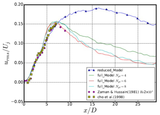
Figure 4.
Influence of the model complexity on the axial velocity fluctuations along the jet axis.
8. Transport of a Passive Scalar
In this paper we consider the case with the change of the density and viscosity happens due to mixing of different species without chemical reaction. The problems under consideration are formulated in terms of the mass fraction of any of the k species, the temperature T, or, the mixture fraction f which transport is described by the equation:
where is the diffusion coefficient that in general depends on both temperature and species composition. The passive scalar fluctuations , are directly resolved in the extended VLES approach, as shown below.
In the same manner as for the velocity field we decompose the scalar f into large and fine scales using the LES filtering. The decomposed form of (41) reads
The Equation (42) is solved on the grid, whereas the second Equation (43) is treated by the scalar particle method with the particles represented in the form
where is the scalar particle size, is the particle strength and is the particle center. Numerical procedure for the calculation of the term is the same as that for the calculation of the term in VLES.
The last Equation (43) is treated in the form:
The first diffusion on the r.h.s of (45) can be treated using the core spreading method with remaining constant. The gradient is calculated by the analytical differentiating (44). Trajectories of the scalar particles are calculated from (23).
In cases of no reaction, the temperature transport equation has the same form as the mixture fraction Equation (41) and can similarly be decomposed.
The mixture fraction formalism allows to reduce the number of particle sets to three sets: vortex particles carrying the vorticity, scalar particles carrying the mixture fraction, species concentration and as well as the scalar particles responsible for the temperature and .
The method can principally be extended to more complex chemical reactions.
9. Boundary Conditions
The boundary conditions (BC) are explicitly formulated only for the grid solution. There are no boundary conditions for the vortex method. For instance, the no slip BC for the velocity can be written in the form [1]
The necessary and sufficient boundary condition for the pressure in incompressible case, which is used in the Poisson equation within pressure correction approaches, is the Neumann BC obtained by the projection of the Equation (3) onto the normal direction [1]:
where the term proportional to the kinematic viscosity was traditionally neglected. Similar BC can be derived for the scalar field and for flows with variable transport properties. We don’t derive these BC and use the traditional BC for the grid based solution from the following considerations:
- Close to the wall the flow is rather smooth and the creation of energetically important concentrated fine structures is unlikely.
- Representation of the continuously spatially distributed structures by discrete particles with a primitive spatial spherical distribution of vorticity results in a serious approximation error and cause numerical instability.
- This approximation can be not physical if the vorticity induced by a particle is not zero beneath the wall , where y is the distance from the wall (see Figure 5). This case takes place when the elongated cells with , where x is the coordinate along the wall, are usually used. In this case the vortex radius . If the vortex is located to the wall closer than the particle approximation of vorticity is fully wrong.
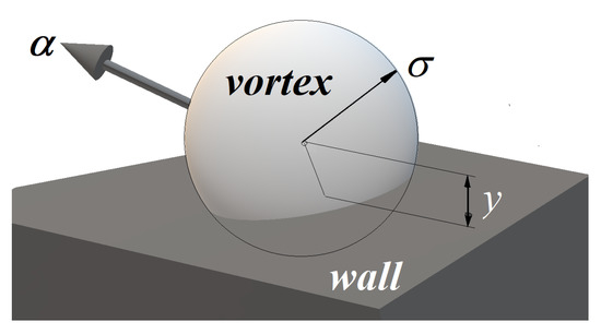 Figure 5. Wrong approximation of the vorticity by a vortex particle when the distance from the wall y is less than the vortex particle radius .
To avoid these difficulties and taking into account the fact, that the influence radius of the vortex particle (area of a sufficient induced velocity ) is approximately we don’t allow the particle generation at the distances introducing the security zone schematically shown in Figure 1. The width of the zone depends on the grid and covers a few grid wall layers in vertical direction. Since the influence of particles at the boundary in such a way is avoided, we use traditional BC for the grid part of the solution. The same procedure is valid for the scalar particles.
10. Implementation of the Method
The coupling of the Particle Method with the existing implicit codes is performed in an explicit way. The terms , and taking into account the influence of fine scales on large ones are taken from the previous time step. Following the particle method, the partial differential Equations (15) and (43) are reduced to the ordinary differential Equations (23), (24), (31), (32), (34), (35), (37) and (45) which are solved using the simple Euler approach, i.e., the r.h.s are taken from the previous time step. Higher order methods like Runge- Kutta or Bashforth- Adams are not necessary, because as mentioned in Section 7, the particles play the trigger role and the accuracy of their inner dynamics calculation is not important.
The full solution takes place in the following order employing the OpenFOAM (OF) code:
- General structure of the time loop in OpenFOAM. Steps 2–5 and 6–11 are additional routines implemented into OpenFOAM (OF).1. Calculation of velocities , pressure and density from (19) and (20) using OpenFoam. is taken from the previous time step.2. Vortex particles identification (see Section 2.1).3. Update of particle positions and strengths (see the Fine Vortex Part below).4. Computation of the term for each cell. is taken from OF.5. Mapping vortex particles onto grid if their size , where is a free scheme parameter, ( in [2,3]).6. Computation of the expansion velocity .7. Calculation of the scalar from (42) using OpenFoam. is taken from the previous time step.8. Scalar particles identification using a similar algorithm for the vorticity (see Section 2.1). Instead of and , and are to utilized. The procedure is performed for two sets of scalar particles. See steps 7.1–7.6.9. Update of scalar particle positions and strengths (see the Fine Scalar Part below, steps 8.1–8.5).10. Computation of the term for each cell. is taken from OF.11. Mapping scalar particles onto grid if their size .12. Calculation of chemical species concentrations using the mixture-fraction presumed PDF approach and fluctuations .13. Calculation of density fluctuations .
- Flowchart of the vortex particle identification procedure. BS stands for Biot- Savart law.The description of this algorithmic step is thoroughly described in Section 2.1.
- Flowchart of the scalar particle identification procedure.7.1 Filtration of and calculation of pulsations7.2 Determination of at cell centers and selection of active cells at which , where is a free scheme parameter to be found in methodological simulations.7.3 Clusters elimination.7.4 Scalar particle is placed at each j-th cell if the cell doesn’t belong to any cluster and . The size and particle strength are and .7.5 At each cell weakest particles are deleted if . is the maximum number of particles in each cell.7.6 Scalar induced by particles is calculated at grid points using (44) and subtracted from the grid scalar . This ensures the conservation of the scalar.
- Fine Vortex Part calculates:3.1 Velocities and tensor at vortex centers from the BS law.3.2 Velocities and tensor at vortex centers from OF.3.3 Vortex displacement from equation .3.4 Change of the vorticity strength magnitude at vortex centers from (15).3.5 Change of from (24).3.6 Particle length from (31).3.7 Particle core radius from (32).3.8 Calculation of the particle core spreading using Core Spreading Method (33).3.9 New particle orientation from (34).3.10 Particle strength magnitude from (35).3.11 New strength vector from (37).3.12 At each cell weakest vortices are deleted if .
- Fine Scalar Part calculates:8.1 tensor at vortex centers from OF.8.2 Particle displacement from equation .8.3 Change of the scalar strength magnitude at particle centers from (45) without the diffusion term.8.4 Calculation of the particle core spreading using Core Spreading Method (33).8.5 At each cell weakest particles are deleted if . Their scalar value is redistributed among neighboring cell centers to ensure the conservation of the scalar.
11. Conclusions
The paper presents the theoretical background of the hybrid grid- based and grid- free method which is the extension of the VLES method, developed originally for incompressible flows, to flows with variable density and transport properties. The method is based on the decomposition of flow parameters into large scale and fine scale parts. The governing equations are obtained through the substitution of this decomposition into the transport equations for vorticity, scalar dynamics and continuity equations. This results in the splitting of transport equations according to scales. Fine scale dynamics is simulated with Lagrangian grid free Particle Method. The numerical approach is designed so that the strengths and the weaknesses of grid-based and grid-free schemes can be seen as complementary. Particle methods are suitable for modeling of fine and fast vortices because they possess a low artificial viscosity, keep vortex particles from excessive diffusion and has no restrictions to Courant number.
The derivations are presented on the level of formulas and algorithms which can directly be implemented into the software code. The overall method is designed so that it can be incorporated into the existing grid based powerful codes like OpenFOAM which have extensive modeling capabilities of multi physical processes.
Author Contributions
Two authors N.K. and J.D. contributed equally to derivation and proof of the theoretical basis of the VLES method extended to flows with variable density and viscosity. S.S. performed simulations presented in Section 7. All authors have read and agreed to the published version of the manuscript.
Funding
This research received no external funding.
Conflicts of Interest
The authors declare no conflict of interest.
Abbreviations
The following abbreviations are used in this manuscript:
| CFD | Computational Fluid Dynamics |
| CSM | Core Spreading Method |
| LES | Large Eddy Simulation |
| OF | OpenFOAM |
| SG | Subgrid |
| VPM | Vortex Particle Method |
References
- Kornev, N. Hybrid Method Based on Embedded Coupled Simulation of Vortex Particles in Grid Based Solution. Comput. Part. Mech. 2018, 5, 269–283. [Google Scholar] [CrossRef]
- Kornev, N.; Samarbakhsh, S. Large Eddy Simulation with direct resolution of subgrid motion using a grid free vortex particle method. Int. J. Heat Fluid Flow 2019, 75, 86–102. [Google Scholar] [CrossRef]
- Samarbakhsh, S.; Kornev, N. Simulation of the free jet using the vortex particle intensified LES (VπLES). Int. J. Heat Fluid Flow 2019, 80, 108489. [Google Scholar] [CrossRef]
- Schlegel, F.; Ghoniem, A. Simulation of a high Reynolds number reactive transverse jet and the formation of a triple flame. Combust. Flame 2014, 161, 971–986. [Google Scholar] [CrossRef]
- Chakraborty, P.; Balachandar, S.; Adrian, R. On the relationships between local vortex identification schemes. J. Fluid Mech. 2005, 535, 189–214. [Google Scholar] [CrossRef]
- Kolar, V. Compressibility effect in vortex identification. AIAA J. 2012, 47, 473–475. [Google Scholar] [CrossRef]
- Landau, L.D.; Lifshitz, E.M. Fluid Mechanics—Course of Theoretical Physics; Institute of Physical Problems, Pergamon Press: Oxford, UK, 1966. [Google Scholar]
- Abdelsamie, A.; Fru, G.; Oster, T.; Dietzsch, F.; Janiga, G.; Thévenin, D. Towards direct numerical simulations of low-Mach number turbulent reacting and two- phase flows using immersed boundaries. Comput. Fluids 2016, 131, 123–141. [Google Scholar] [CrossRef]
- Weinan, E. Principles of Multiscale Modeling; Cambridge University Press: Cambridge, UK, 2011. [Google Scholar]
- Tabak, E. Vortex Stretching in Incompressible and Compressible Fluids; Fluid Dynamics II Course; Mathematical Department, New York University: New York, NY, USA, 2002; 10p. [Google Scholar]
- Fukuda, K.; Kamemoto, K. Application of a Redistribution Model Incorporated in a Vortex Method to Turbulent Flow Analysis. In Proceedings of the 3rd International Conference on Vortex Flows and Vortex Models (ICVFM2005), Yokohama, Japan, 21–23 November 2005. [Google Scholar]
- Cottet, G.H.; Koumotsakos, P.D. Vortex Methods: Theory and Practice; Cambridge University Press: Cambridge, UK, 2000. [Google Scholar]
© 2020 by the authors. Licensee MDPI, Basel, Switzerland. This article is an open access article distributed under the terms and conditions of the Creative Commons Attribution (CC BY) license (http://creativecommons.org/licenses/by/4.0/).