Three-Dimensional Convective Planforms for Inclined Darcy-Bénard Convection

Abstract

We investigate the onset of convection in an inclined Darcy-Bénard layer. When such a layer is unbounded in the spanwise direction it is generally known that longitudinal rolls comprise the most unstable planform. On the other hand, when a layer has a sufficiently small spanwise width, then transverse rolls form the most unstable planform. However, the layer remains stable to transverse roll disturbances when the inclination is above roughly 31 degrees from the horizontal. This paper considers the transition between these two extreme cases where the spanwise width takes moderate values and where rectangular cells are considered. It is found that the most unstable planform is quite strongly sensitive to the magnitude of the spanwise width and that there are large regions of parameter space within which three-dimensional convection patterns have the smallest critical Darcy-Rayleigh number.

1. Introduction

The Rayleigh-Bénard instability in a porous layer saturated by a fluid and heated from below has been the subject of many investigations over the last decades. A thorough and updated survey of the most important results in this field can be found in the book by Nield and Bejan [1]. The alternative name used for this instability when a porous medium is involved is Darcy-Bénard as the momentum transfer for seepage flows is modelled through Darcy’s law. Usually, the porous layer where the thermoconvective instability arises in the form of cellular patterns is assumed to be horizontal and bounded by impermeable walls kept at different uniform temperatures. This situation has a stationary basic state where no flow occurs and a vertical temperature gradient directed downward causes the instability. There is a different scenario when the porous layer is inclined at an angle $\alpha$ to the horizontal. In this case, the basic seepage velocity is a parallel vector field with a non-uniform linear profile yielding a longitudinal flow with zero net rate.

Pioneering studies of the Darcy-Bénard problem in an inclined porous layer were carried out by Bories and Combarnous [2] and by Weber [3]. The main consequence of the inclination is that the critical Rayleigh number at the onset of the instability depends on the inclination $\alpha$ through a factor $1/cos\alpha$. The ultimate effect of this factor is that no convective instability can arise when the porous layer becomes vertical $(\alpha ={90}^{\circ })$. A rigorous analysis of this effect is reported in a short paper by Gill [4]. The consequences of Gill’s no-go theorem for the instability in a vertical layer were studied further by Lewis, Bassom and Rees [5] using asymptotic theory and by Straughan [6] using nonlinear stability theory. It must be mentioned that the scaling of the critical Rayleigh number through the factor $1/cos\alpha$ holds whenever the most unstable modes at onset are longitudinal rolls. This is the typical situation when the inclined porous layer has no lateral confinement. On the other hand, the effect of lateral confinement implies the emergence of transverse rolls as the preferred modes activating the instability (Rees and Bassom [7]), when the distance between the confining sidewalls is very narrow. As shown by Rees and Bassom [7], a peculiarity of unstable transverse rolls is their disappearance when the inclination of the porous layer exceeds the threshold angle $\alpha ={31.49032}^{\circ }$.

Further studies of the Darcy-Bénard instability in an inclined porous layer have been carried out, for instance, by Postelnicu and Rees [8], Rees and Postelnicu [9], Rees, Postelnicu and Storesletten [10], Rees, Storesletten and Postelnicu [11], Barletta and Rees [12]. Such studies were mainly concerned with the model employed to describe the flow and the heat transfer in the porous medium either by including the anisotropy of the porous material, or inertial effects, or the local thermal non-equilibrium within the saturated medium. Further investigations were focussed on alternative types of temperature and velocity conditions employed to model the inclined plane boundaries which, in the classical Darcy-Bénard problem, are assumed as impermeable and isothermal. This is the case of the papers by Barletta and Storesletten [13], Rees and Barletta [14], Barletta and Rees [15], Barletta and Celli [16], Celli and Barletta [17]. Further recent studies have been reported by Rees and Bassom [18] and by Wen and Chini [19]. In the former paper, the boundary layer regime is analysed for a porous medium heated from below through an inclined isothermal boundary with uniform suction. In the latter paper, a nonlinear analysis of transverse rolls is performed for Darcy-Bénard convection in an inclined porous layer where it is shown that it is possible to obtain strongly nonlinear convection at inclinations greater than the above-mentioned ${31.49032}^{\circ }$. We also mention the early work by Riley and Winters [20] who undertook a bifurcation analysis of transverse cells in an inclined finite porous cavity.

The aim of this paper is to extend the linear analysis of the onset of instability carried out by Rees and Bassom [7] who considered a two-dimensional model of the instability as driven by transverse rolls. When there is a lateral confinement where the distance between the sidewalls is not too small then it may be possible for three-dimensional modes to arise at onset of convection. Such modes will correspond to rectangular planforms and these are equivalent to the sum of two otherwise identical oblique rolls aligned at equal but opposite directions from that of a longitudinal roll. A general modal map of the onset of instability in the inclined porous layer is provided for different inclinations, $\alpha$, and aspect ratios of the transverse cross-section of the layer. The analysis is carried out numerically by employing a shooting-method solution of the stability eigenvalue problem. A perturbation analysis is also presented providing some analytical results for the transition between longitudinal rolls and oblique rolls forming the preferred pattern of convection.

2. Governing Equations and Stability Analysis

The aim is to investigate the effect of the presence of sidewalls on the onset of convective instability for the inclined Darcy-Bénard problem. Specifically the intention is to determine the identity of the most unstable mode without being restricted solely to transverse or longitudinal rolls. The nondimensional governing equations are

$${\displaystyle \frac{\partial u}{\partial x}}+{\displaystyle \frac{\partial v}{\partial y}}+{\displaystyle \frac{\partial w}{\partial z}}=0,$$

(1)

$$u=-{\displaystyle \frac{\partial p}{\partial x}}+(\mathrm{Ra}sin\alpha )(\theta -\frac{1}{2}),$$

(2)

$$v=-{\displaystyle \frac{\partial p}{\partial y}}+(\mathrm{Ra}cos\alpha )(\theta -\frac{1}{2}),$$

(3)

$$w=-{\displaystyle \frac{\partial p}{\partial z}},$$

(4)

$${\displaystyle \frac{\partial \theta }{\partial t}}+u{\displaystyle \frac{\partial \theta }{\partial x}}+v{\displaystyle \frac{\partial \theta }{\partial y}}+w{\displaystyle \frac{\partial \theta }{\partial z}}={\displaystyle \frac{{\partial }^2\theta }{\partial x^2}}+{\displaystyle \frac{{\partial }^2\theta }{\partial y^2}}+{\displaystyle \frac{{\partial }^2\theta }{\partial z^2}},$$

(5)

where z is a horizontal coordinate and where $\alpha$ is the angle of rotation of the layer about the z-axis. In addition, y is the coordinate which acts in the normal direction to the heated surfaces, and x is the coordinate up the layer. The above equations form the standard set for problems of this type, and the Darcy-Rayleigh number, $\mathrm{Ra}$, is given by

$$\mathrm{Ra}={\displaystyle \frac{\rho g\beta Kd\Delta T}{\mu \kappa }},$$

(6)

where d is the thickness of the uniform layer where $\rho$ is the reference density, g the strength of gravity, $\beta$ the coefficient of cubical expansion, $\Delta T$ the temperture drop across the layer, $\mu$ the dynamic viscosity, and $\kappa$ the thermal diffusivity of the porous medium. The boundary conditions which are required to complete the specification of the problem are,

$$v=0,\theta =1\mathrm{on}y=0,v=0,\theta =0\mathrm{on}y=1,w=0,{\displaystyle \frac{\partial \theta }{\partial z}}=0\mathrm{on}z=0,L.$$

(7)

We note that the conditions on the spanwise sidewalls at $z=0,L$ also imply that $\partial p/\partial z=0$ there.

From these equations we see that the basic state, whose stability forms the subject of the paper, is given by,

$$\theta =1-y,u=\mathrm{Ra}sin\alpha (\frac{1}{2}-y),v=w=0,{\displaystyle \frac{\partial p}{\partial y}}=\mathrm{Ra}cos\alpha (\frac{1}{2}-y).$$

(8)

These profiles may be subtracted out of the governing equations and the resulting system is then linearised. Equations (1) to (4) then remain unchanged, but Equation (5) takes the form,

$${\displaystyle \frac{\partial \theta }{\partial t}}+(\mathrm{Ra}sin\alpha )(\frac{1}{2}-y){\displaystyle \frac{\partial \theta }{\partial x}}-v={\displaystyle \frac{{\partial }^2\theta }{\partial x^2}}+{\displaystyle \frac{{\partial }^2\theta }{\partial y^2}}+{\displaystyle \frac{{\partial }^2\theta }{\partial z^2}}.$$

(9)

The velocity components may now be removed and the resulting pair of equations in pressure/temperature form are,

$${\displaystyle \frac{{\partial }^{2}p}{\partial x^2}}+{\displaystyle \frac{{\partial }^{2}p}{\partial y^2}}+{\displaystyle \frac{{\partial }^{2}p}{\partial z^2}}=(\mathrm{Ra}sin\alpha ){\displaystyle \frac{\partial \theta }{\partial x}}+(\mathrm{Ra}cos\alpha ){\displaystyle \frac{\partial \theta }{\partial y}},$$

(10)

$${\displaystyle \frac{\partial \theta }{\partial t}}+(\mathrm{Ra}sin\alpha )(\frac{1}{2}-y){\displaystyle \frac{\partial \theta }{\partial x}}-(\mathrm{Ra}cos\alpha )\theta +{\displaystyle \frac{\partial p}{\partial y}}={\displaystyle \frac{{\partial }^2\theta }{\partial x^2}}+{\displaystyle \frac{{\partial }^2\theta }{\partial y^2}}+{\displaystyle \frac{{\partial }^2\theta }{\partial z^2}}.$$

(11)

The boundary conditions are now that,

$${\displaystyle \frac{\partial p}{\partial y}}=\theta =0\mathrm{on}y=0,1,{\displaystyle \frac{\partial p}{\partial z}}={\displaystyle \frac{\partial \theta }{\partial z}}=0\mathrm{on}z=0,L.$$

(12)

We shall consider three-dimensional disturbances which are proportional to $cos(n\pi z/L)$, i.e., where n rolls have been fitted into the spanwise width of the layer. This form may be used for both the pressure and the temperature because each satisfies a zero Neumann condition at the sidewalls. However, there also needs to be a component in the x-direction in order to allow for the presence of three-dimensional convection, and therefore we may take the disturbance temperature field to be proportional to $cos(n\pi z/L)cos\left(mx\right)$ where m is a wavenumber. This product of cosines, which represents convection with a rectangular planform, may also be split into the sum of two independent oblique rolls,

$$cos(n\pi z/L)cos\left(mx\right)=\frac{1}{4}\left[e^{i(n\pi z/L-mx)}+e^{i(n\pi z/L+mx)}\right]+\mathrm{complex}\mathrm{conjugate},$$

(13)

which are equally inclined away from the direction of the x-axis but in opposite directions. We note that it is sufficient to consider just one of these rolls since the other has identical stability properties. Therefore in the rest of the paper we shall refer to an oblique roll disturbance as a proxy for the 3D cell with the rectangular planform given that it may be visualised easily.

The presentation of the stability analysis is made easier by defining an overall wavenumber, k, where k is given by,

$$e^{i(n\pi z/L-mx)}=e^{ik(zcos\varphi -xsin\varphi )}.$$

(14)

and where $\varphi$ is its orientation. We note that $\varphi =0$ corresponds to longitudinal rolls, and $\varphi =\pi /2$ to transverse rolls (although such rolls will also require $n=0$). Although our computations will use k, it is the spanwise width, L, and the nuber of cells, n, which are imposed on the configuration. Therefore we have,

$$k={\displaystyle \frac{n\pi }{Lcos\varphi }};$$

(15)

this dependence of k on $\varphi$ will be relied upon later. Therefore we shall take the following form for the disturbances,

$$\left(\begin{array}{c}p\\ \theta \end{array}\right)=e^{ik(zcos\varphi -xsin\varphi )+\lambda t}\left(\begin{array}{c}f\left(y\right)\\ g\left(y\right)\end{array}\right)+\mathrm{complex}\mathrm{conjugate},$$

(16)

where $\lambda ={\lambda }_r+i{\lambda }_i$ is the complex exponential growth rate. The functions $f\left(y\right)$ and $g\left(y\right)$ satisfy,

$$f^{″}-k^{2}f=(\mathrm{Ra}cos\alpha )g^{\prime }-(ik\mathrm{Ra}sin\alpha sin\varphi )g,$$

(17)

$$g^{″}-k^{2}g=f^{\prime }-(\mathrm{Ra}cos\alpha )g-(ik\mathrm{Ra}sin\alpha sin\varphi )(\frac{1}{2}-y)g+\lambda g.$$

(18)

This will be treated as an eigenvalue problem for both $\mathrm{Ra}$ and ${\lambda }_i$ where ${\lambda }_r=0$ is imposed and which corresponds to marginal stability. The boundary conditions are taken to be,

$$f^{\prime }\left(0\right)=f^{\prime }\left(1\right)=g\left(0\right)=g\left(1\right)\mathrm{and}{g}^{\prime }\left(0\right)=1,$$

(19)

where the last condition is a normalisation condition. This complex eigenvalue problem was solved using a fourth order Runge Kutta method as part of a shooting method code. Computations made with this code, which uses a pressure/temperature formulation, compare perfectly with those of Rees and Bassom [7] who used a streamfunction/temperature formulation.

Table 1. Accuracy tests for the given cases with $n=1$.

	$\mathit{L}=1,\mathit{\alpha }=0,\mathit{\varphi }=0$		$\mathit{L}=1.2,\mathit{\alpha }{=25}^{\circ },\mathit{\varphi }{=10}^{\circ }$
N	${\mathrm{Ra}}_{\mathbf{c}}\left(\mathbf{N}\right)$	Error	${\mathrm{Ra}}_c\left(\mathbf{N}\right)$	Error
25	$39.47858076$	0.000 163 16	45.024 341 41	0.000 201 46
50	$39.47842784$	0.000 010 24	45.024 152 58	0.000 012 63
100	$39.47841825$	0.000 000 65	45.024 140 74	0.000 000 79
200	$39.47841764$	0.000 000 04	45.024 140 00	0.000 000 05
400	$39.47841761$	0.000 000 00	45.024 139 95	0.000 000 00
800	$39.47841761$	0.000 000 00	45.024 139 95	0.000 000 00

shows how the computed values of the critical Darcy-Rayleigh number vary with successive interval-halving where N is the number of uniform intervals. Two different cases are presented and they demonstrate that the numerical errors reduce by a factor of roughly $2^4$ as the intervals are halved, which also confirms the 4th order accuracy of the method. We have therefore decided to use a uniform grid of 100 intervals in all of our computations; this may be seen to provide eight significant figures of accuracy.

It is important to note that while some of the computations presented in Rees and Bassom [7] correspond to travelling modes, i.e., they correspond to nonzero values of ${\lambda }_i$, these cases arise in regions of parameter space which are quite distant from where the minima in the neutral curves are located. Therefore the present computations, which are concerned with such minima, always give rise to stationary modes for which ${\lambda }_i=0$.

3. Results and Discussion

The ultimate aim is to provide an informative modal map in the spirit of Beck’s well-known analysis of Darcy-Bénard convection in a cuboid [21]. This will show the preferred planform for convection at onset as a function of both the spanwise width of the layer and the inclination angle. We shall begin with an attempt to understand how the neutral curves vary with the governing parameters.

3.1. Sample Neutral Curves

The four subfigures which comprise Figure 1 display how the critical Darcy-Rayleigh number varies with the roll orientation, $\varphi$ for the inclination angle, $\alpha =5^{\circ }$. The subfigures are distinguished by having different numbers of rolls occupying the layer. In all cases the equivalent critical Darcy-Rayleigh number for the transverse mode is given by the blue line. A rather large number of curves are displayed here and it is impractical to attempt to label them. Therefore the manner in which the curves have been plotted serves to identify the values of L. Thus red curves correspond to values of L which are less than n, and dashed curves denote cases where L is an integer. The right-most curve corresponds to $L=5$. Therefore, in all four cases shown, the curve with the lowest minimum value may be seen to correspond to when $L=n$, given that it is dashed and is the first instance of a black curve as one moves to the right. In fact, each of the $L=n$ curves shown have identical shapes because of the form of Equation (15) which means that the linear stability equations are solved using precisely the same value of k. This observation may also be generalised to saying that any two cases with identical values of $n/L$, $\varphi$ and $\alpha$ are identical mathematically and have the same critical Darcy-Rayleigh number.

We note that the curves corresponding to different widths, L, always have their minimum below the critical value of $\mathrm{Ra}$ for transverse rolls, and therefore we do not expect transverse rolls to form the most unstable mode unless the layer is sufficiently narrow, i.e., unless L is sufficiently small. In addition, the roll orientation is not always that of the longitudinal roll ($\varphi =0$), but $\varphi$ often takes nonzero values and corresponds to an oblique mode.

We mention that the locus of the minima as L increases continuously traces the same curve independently of the value of n, and this will also be true for a similar set of curves for different inclinations. Therefore we shall not present such a large amount of data for other inclination.

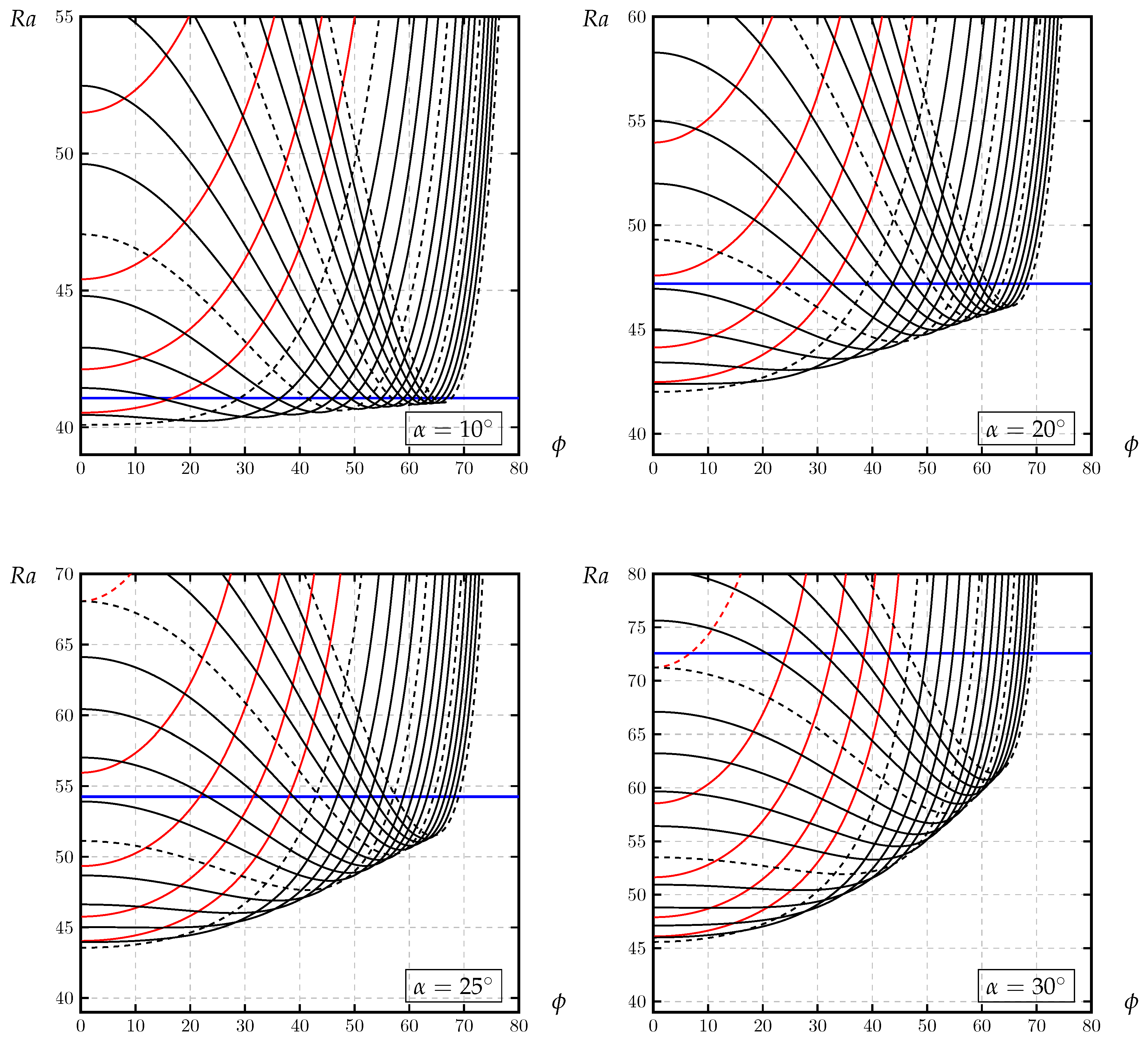
Figure 2 shows how such neutral curves vary with the inclination angle, and we have chosen the 2-roll case, $n=2$, for these. The main general observation is that the Darcy-Rayleigh number increases with increasing inclination, should n, L and $\varphi$ be held fixed, and this also includes the transverse roll. Yet again, for any chosen value of L and $\alpha$ the minimum value of the Darcy-Rayleigh number lies below that of the transverse roll, and it may or may not correspond to $\varphi =0$.

Let us consider, for example, the $\alpha ={10}^{\circ }$ case, and specifically at the two black curves which intersect the vertical axis one moves upwards from $\mathrm{Ra}=40$. The dashed line, which corresponds to $L=2$, has its minimum at $\varphi =0$ and therefore it is a longitudinal roll. The second curve, a continuous curve, has its minimum at $\varphi \simeq {22}^{\circ }$ and is an oblique roll. Therefore this is a case where neither the transverse nor the longintudinal roll forms the preferred mode, a situation which, as will be seen, is quite common for low inclinations.

Curves for $L>5$ follow the same trend, namely that their minima correspond to increasing values of both $\mathrm{Ra}$ and $\varphi$. In fact $\mathrm{Ra}$ will never exceed the value for the tranverse roll while $\varphi$ tends towards ${90}^{\circ }$.

In Figure 3 neutral curves are shown again but from a different point of view. We have taken the inclination $\alpha ={20}^{\circ }$ to represent a typical case, and have concentrated on aspect ratios varying in steps of $0.2$ from $L=3$ to $L=4$. The different curves correspond to different values of n and these are colour-coded in the manner defined in the caption.

When $L=3$, the preferred mode is the $n=3$ mode which is displayed in red. When L increases to $3.2$, the various minima in the curves tend to move either to the right (when $\varphi$ is nonzero) or downwards (when $\varphi$ is zero). This process continues in the same way except that when $L=3.4$, the red $n=3$ curve now has a local maximum at $\varphi =0$ and the global minimum, which is difficult to see in the figure, is at $\varphi \simeq {25.8}^{\circ }$. Therefore the preferred mode is now an oblique roll. At $L=3.6$ the critical Darcy-Rayleigh number for the $n=3$ longitudinal is now larger than that for the $n=4$ roll, shown in purple. However, the oblique $n=3$ mode remains the preferred pattern. When $L=3.8$ and $L=4$, the $n=4$ longitudinal roll assumes the role of being the most dangerous.

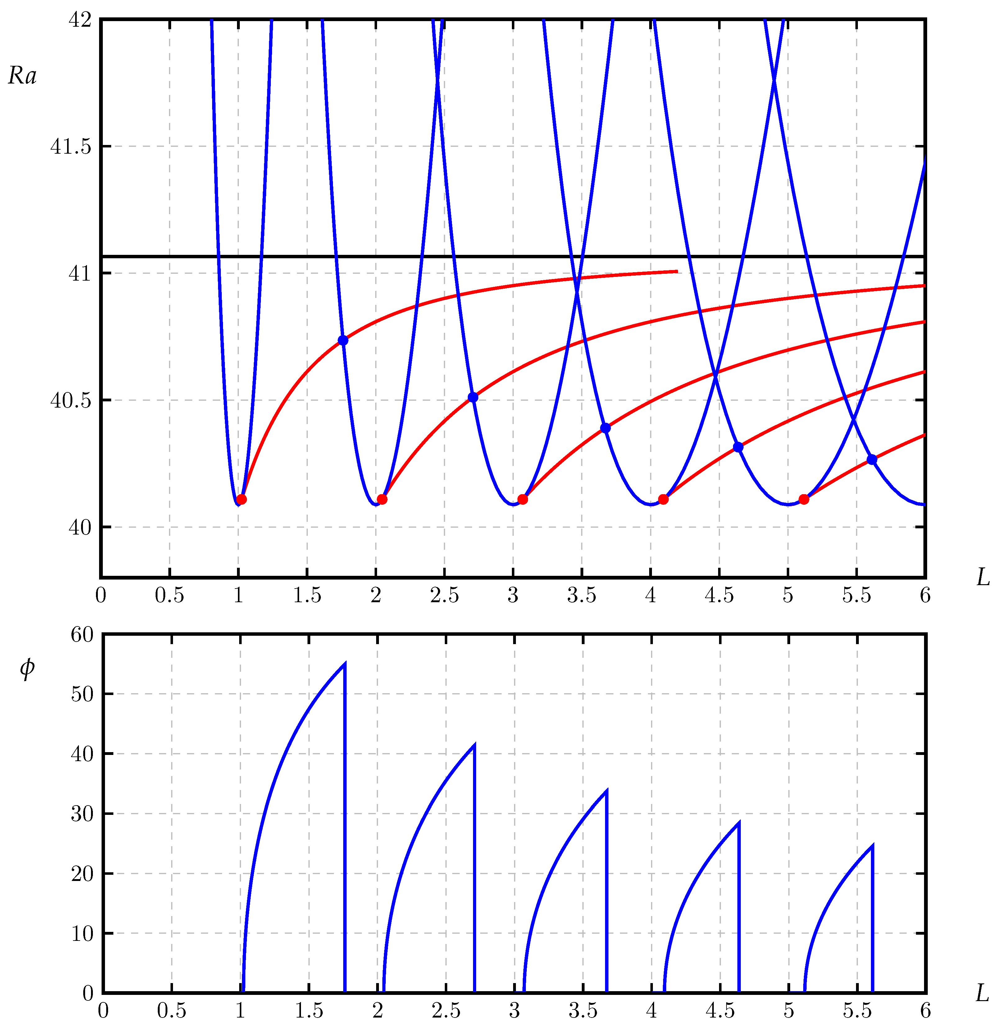
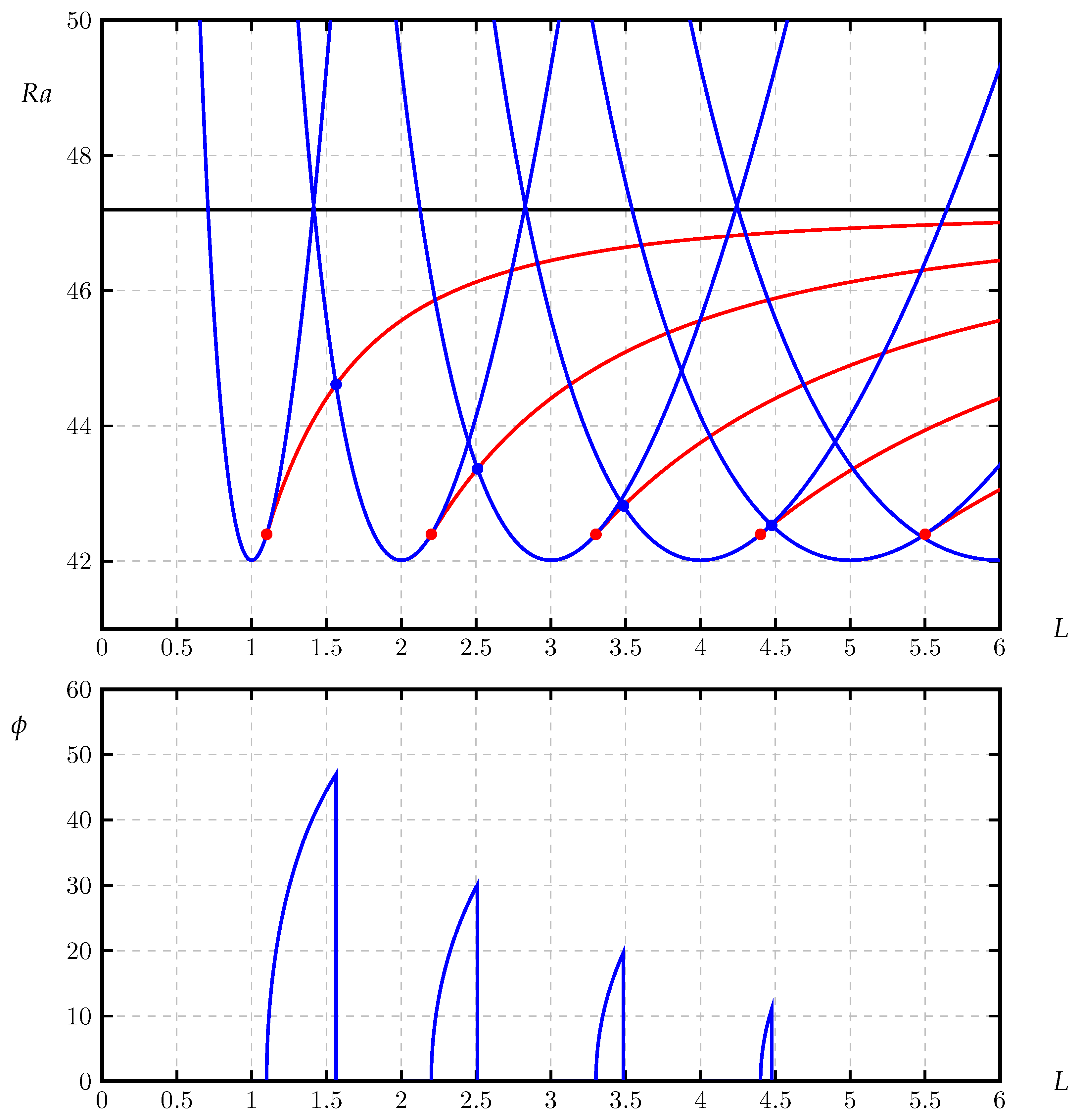
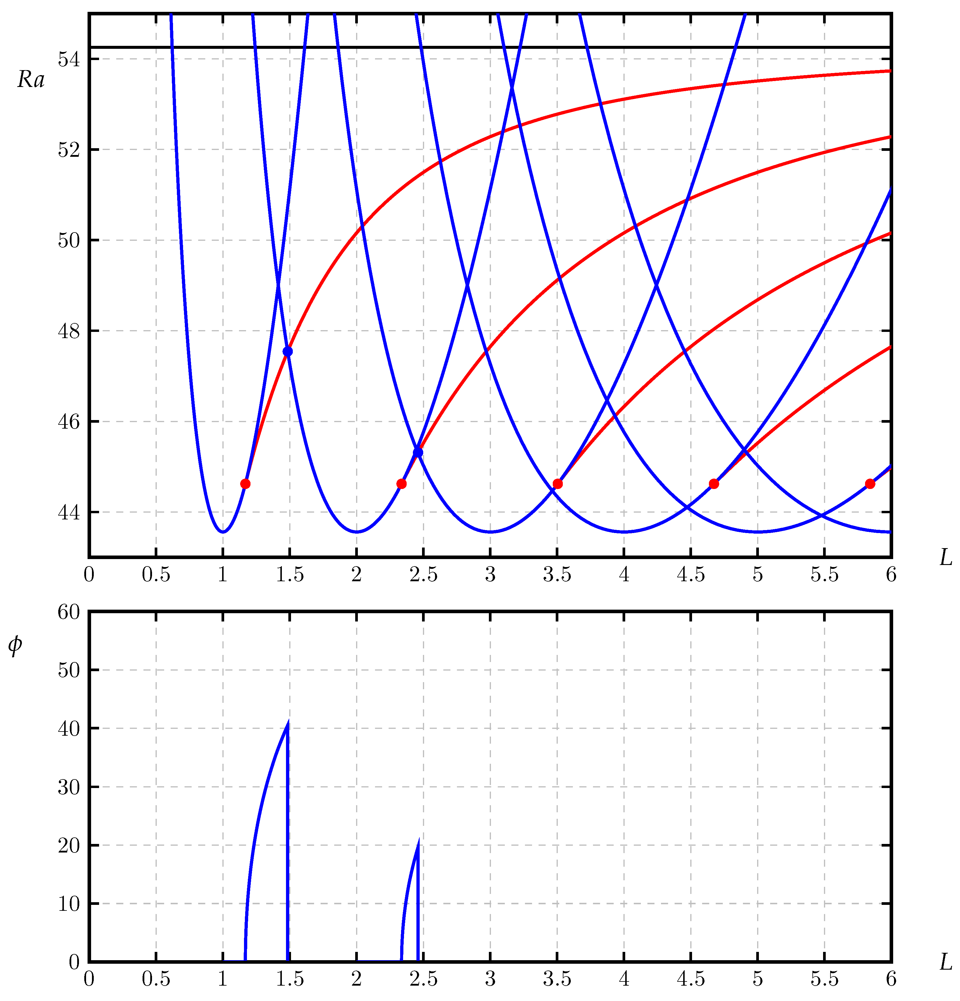
Although we have chosen to consider this transition using the case $\alpha ={20}^{\circ }$ and when L varies between 3 and 4, this scenario is ubiquitous. There are two exceptions, however: (i) when L is sufficiently far below 1 that transverse rolls are favoured, and (ii) when the inclination is sufficently large. So Figure 4, Figure 5 and Figure 6 begin the the process of understanding the global picture of the linear stability properties of this system. These figures, which correspond respectively to $\alpha ={10}^{\circ }$, $\alpha ={20}^{\circ }$ and $\alpha ={25}^{\circ }$, show how the critical Darcy-Rayleigh number and the roll orientation varies with aspect ratio, L. In the Darcy-Rayleigh number plots we show curves for transverse, longitudinal and oblique rolls.

The blue curves denote longitudinal rolls, and in Figure 4, for the longitudinal mode which has its minimum at $L=1$, it needs only a very slight increase in L from $L=1$ to $L=1.023303$ for the longitudinal mode’s variation in $\varphi$ to make the above-mentioned transition from $\varphi =0$ being a minimum to being a local maximum, and then oblique rolls form the preferred planform. The transitional value, $L=1.023303$, may be referred to as a quartic point.

The detailed variation of $\varphi$ with L is shown in the lower part of the figure and it resembles the separate buildings of the Sydney Opera House in its disjointed shape. The sudden transitions in $\varphi$ back to zero correspond to the blue disks in the upper plot where, for example, the $n=1$ red curve crosses the $n=2$ blue curve and the preferred mode changes its identity.

Figure 5 and Figure 6 have similar features except that it becomes clear that there are only a finite number of ‘buildings’ in the Sydney Opera House shape. The reason is that the quartic point for each inclination, the red disks in Figure 4, Figure 5 and Figure 6, all occur at the same value of the Darcy-Rayleigh number, while the intersections between the curves corresponding to neighbouring longitudinal mode curves occur at decreasing values of the Darcy-Rayleigh number. So for $\alpha ={20}^{\circ }$ there are four disconnected ranges of values of L for which oblique modes arise, while for $\alpha ={25}^{\circ }$ it is only two, and for $\alpha ={30}^{\circ }$, which is not shown here, it is just the one.

It is possible to determine quite easily what happens when $\alpha =0$. The neutral curve for an unbounded horizontal plane layer is given by,

$$\mathrm{Ra}={\displaystyle \frac{{(k^2+{\pi }^2)}^2}{k^2}}$$

(20)

where, for the present bounded problem, k is given by Equation (15). Hence we have,

$$\mathrm{Ra}={\pi }^2{\displaystyle \frac{{(L^2{cos}^2\varphi +n^2)}^2}{n^2{L}^2{cos}^2\varphi }}.$$

(21)

For a given number of rolls, n, this expression is maximised when

$$Lcos\varphi =n\mathrm{or}cos\varphi =n/L,$$

(22)

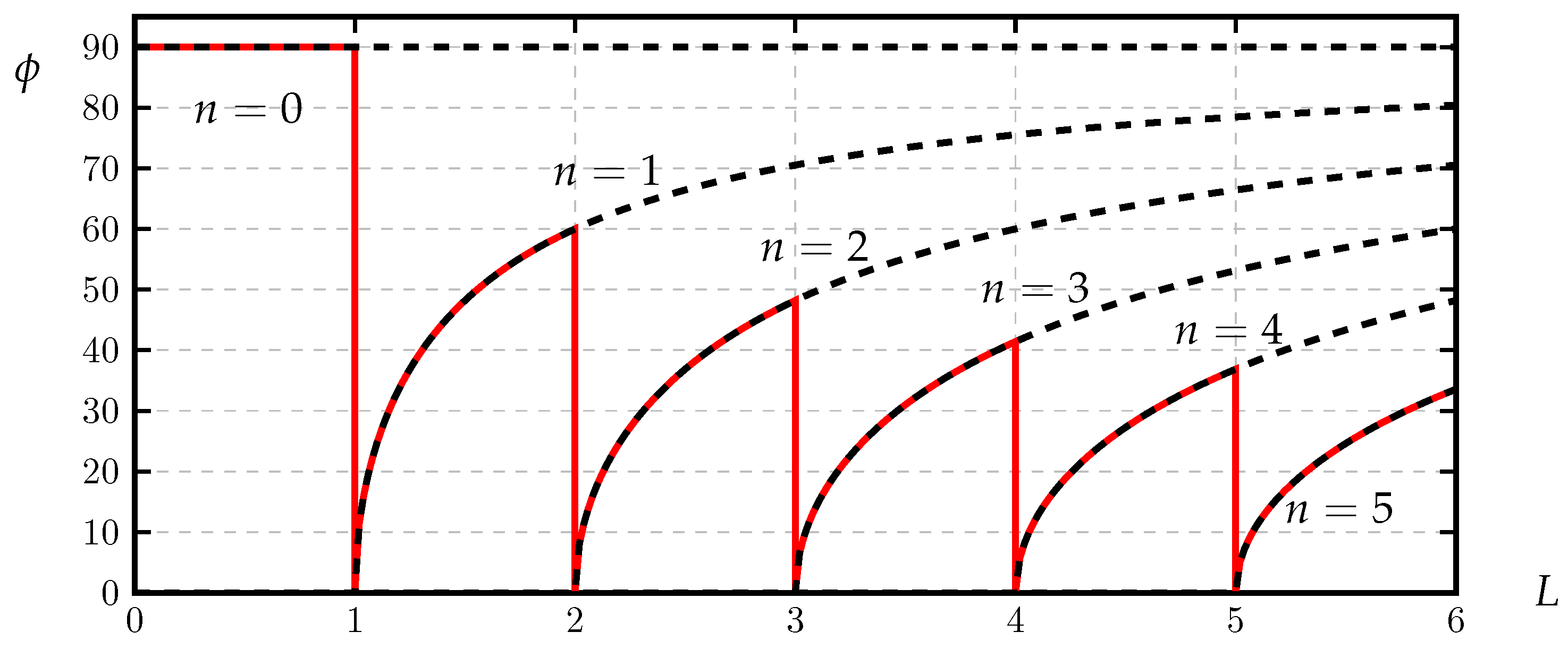
at which point $\mathrm{Ra}=4{\pi }^2$. When L is an integer, the case $n=L$ yields an n-cell longitudinal roll pattern ($\varphi =0$) as the most unstable disturbance; other values of n give larger values of the Darcy-Rayleigh number irrespective of the roll orientation. When L is not an integer, then the most unstable disturbance takes the form of oblique rolls with n cells where n is any integer which is smaller than L. For example, when $L=3.5$, then there are three possible planforms where ${\mathrm{Ra}}_c=4{\pi }^2$, namely $n=1$ ($cos\varphi =1/3.5$), $n=2$ ($cos\varphi =2/3.5$) and $n=3$ ($cos\varphi =3/3.5$). These curves are shown as the black dashed lines in Figure 7 when we see that there will always be a degeneracy whenever $L>2$ by having more than one choice of pattern with the smallest possible critical Darcy-Rayleigh number. Although we shall not prove it here once $\alpha$ rises about zero be it ever so slightly, this degeneracy in the identity of the preferred mode resolves. The unique preferred mode then becomes the one with the largest value of n which is less than L, and this is shown as the red line.

The variation in the orientations of the oblique mode with L for this very slightly-inclined case is shown in Figure 7, and these too resemble the Sydney Opera House shape. Moreover, if one compares the dependence of $\mathsf{\Phi }$ on L as shown in Figure 4, Figure 5 and Figure 6 in that order, then the dependence shown in Figure 7 is clearly seen to be reasonable. One implication of Figure 7 is that longitudinal rolls can only form the preferred onset pattern in a horizontal layer when L is an integer.

3.2. The Modal Map

Finally, we are in a position to provide the modal map which summarises the stability properties of the inclined layer with a finite spanwise width, and this is shown in Figure 8. There are three main regions and these are colour-coded for easy reference. The blue region corresponds to when we expect transverse rolls to appear first as $\mathrm{Ra}$ increases. The region is bounded to the right at $L=1$ and above by $\alpha ={31.49032}^{\circ }$, which is the maximum inclination for linear instability (Rees and Bassom 2000).

The white regions are when longitudinal rolls are preferred. For a randomly chosen value of L, the appearance of longituinal rolls becomes decreasingly likely as the layer tends towards being horizontal, and the ever-decreasing ranges of values of L tend to be focused near integer values of L.

The orange shark fin shapes correspond to when oblique rolls (i.e., rectangular cells) are favoured. The left hand boundaries correspond to when the neutral curves (in terms of $\mathrm{Ra}$ against $\varphi$) have a quartic point, and therefore $\mathrm{Ra}$ satisfies $d^2\mathrm{Ra}/d{\varphi }^2=0$; such locations are shown as the blue disks in Figure 4, Figure 5 and Figure 6. Numerically, this curve was obtained by solving Equations (A6)–(A11) given in the Appendix A (although the Appendix A also provides the analytical solution).

The right hand boundaries correspond to the red disks in those Figures, i.e., where an oblique mode for n rolls has the same critical Darcy-Rayleigh number as a longitudinal mode with $n+1$ rolls. This curve was obtained by solving Equations (5) and (7) together with (A8) and (A9) which guarantees that the minimum in the neutral curve has been obtained. The value of $\alpha$ as a function of L was obtained by adding the further constraint that the oblique mode with n cells has the same critical Darcy-Rayleigh number as the longitudinal mode with $n+1$ cells.

When these two curves meet at the sharp end, both sides of the fin tip represent longitudinal rolls, the left with say n rolls and the right with $n+1$ rolls. This is well-known to take place when $L=\sqrt{n(n+1)}$, for this is what happens for 2D convection in a porous box of aspect ratio, L (cf. p313 of Nield and Bejan 2017).

The Appendix contains a detailed analysis for the left hand sides of the fins, and this provides the following formula relating $\alpha$ to n and L:

$${tan}^2\alpha ={\displaystyle \frac{96n^2{L}^4(L^2-n^2)}{{(L^2+n^2)}^3[({\pi }^2+3)L^2+(15-{\pi }^2)n^2]}}$$

(23)

which compares favourably to 8 significant figures with the numerical calculations shown in Figure 7. When $L=\sqrt{n(n+1)}$ is substituted into Equation (23) we obtain

$${tan}^2\alpha ={\displaystyle \frac{96n{(n+1)}^2}{{(2n+1)}^3(18n+3+{\pi }^2)}},$$

(24)

which gives the value of $\alpha$ at the tip of the fin. For $n=1$ and $n=5$, for example, Equation (24) yields,

$${tan}^2\alpha ={\displaystyle \frac{128}{9(21+{\pi }^2)}}\mathrm{and}{tan}^2\alpha ={\displaystyle \frac{17820}{1331(93+{\pi }^2)}}.$$

(25)

Some numerical data which has been obtained using Equation (24) are given in

Table 2. Inclinations corresponding to the $n^{\mathrm{th}}$ fin tip.

n		$\mathit{\alpha }$(Degrees)
1		$34.167212$
2		$28.006732$
3		$24.143052$
4		$21.499921$
5		$19.557799$
10		$14.306414$
20		$10.288103$
50		$6.572284$
100		$4.662749$

, below.

Table 2 shows that, as L increases, the range of inclinations within which we might observe oblique rolls decreases as the aspect ratio increases. Indeed, it is quite easy to use Equation (24) to show that

$${tan}^2\alpha ={\displaystyle \frac{2}{3n}}+O\left(n^{-2}\right)\mathrm{when}n\gg 1.$$

(26)

We have also presented lines of constant $\varphi$ within the orange regions of Figure 8 to indicate concisely which oblique modes are to be expected. The form of these contours suggests that the maximum possible value of $\varphi$ within any chosen shark fin shape is to be found at the bottom right hand corner. This value of $\varphi$ may be found using Equation (22) using $L=n+1$. Therefore we have,

$$cos\varphi =n/(n+1).$$

(27)

For the left-most shark fin we have $\varphi ={cos}^{-1}(1/2)={60}^{\circ }$ while for the second we have $\varphi ={cos}^{-1}(2/3)={48.1897}^{\circ }$, and so on. As an extreme example, for $n=100$, which is the final entry in Table 2, $\varphi ={cos}^{-1}(100/101)={8.0693}^{\circ }$. Therefore, when L is large, not only is there a small range of $\alpha$ within which which oblique rolls are preferred, but the deviation from the direction of the longitudinal roll is also small.

4. Conclusions

In this paper we have studied the effect of having a spanwise constraint on the onset of Darcy-Bénard convection in an inclined porous layer. When the layer is unconstrained in this way, it is well-known that longitudinal rolls always form the most unstable convection pattern and that the critical Darcy-Rayleigh number is $4{\pi }^2/cos\alpha$. It is also well-known that if the layer is sufficiently well-constrained by having an exceptionally narrow layer then transverse rolls arise. Here we have relaxed the assumption that convection takes either of these two forms by considering cells with a rectangular planform, for which the oblique rolls are a proxy. It has been found that, for moderate values of the aspect ratio, L, and for inclinations which are less than, say, ${30}^{\circ }$, quite a large amount of the $(L,\alpha )$ parameter space corresponds to oblique rolls forming the preferred pattern of convection.

We have been able to provide an analytical expression for when a longitudinal roll loses its dominance to oblique modes as L increases. We have also found a precise expression for when oblique rolls give way to longitudinal rolls as the inclination increases (viz. the apex of the shark fin shapes). Although transverse rolls are well known to be unstable only when $\alpha <{31.49032}^{\circ }$, we have found that it is possible to obtain oblique rolls at slightly higher inclinations than that, although $\alpha =34.167212$ is the upper limit.

If one were to wish to extend this analysis still further by considering an inclined cuboid, then the task will be very substantially more difficult. In the present case the basic state may be written down analytically, while this cuboidal extension will need its basic state computed numerically. But even then, there are complications because the concept of the onset of convection doesn’t always apply (Guerrero-Martínez, Karimi and Ramos [22]). Even when confined to two-dimensional convection, some aspect ratios (typically those where L is close to being an even integer) will exhibit a classical bifurcation from the basic state to a strongly convecting solution, but others (where L is close to being an odd integer) exhibit a smooth transition to strong convection. Another complicating factor is that the work of Wen and Chini [19] has uncovered subcritical onset of convection.

References

1. Nield, D.A.; Bejan, A. Convection in Porous Media, 5th ed.; Springer: New York, NY, USA, 2017. [Google Scholar]
2. Bories, S.A.; Combarnous, M.A. Natural convection in a sloping porous layer. J. Fluid Mech. 1973, 57, 63–79. [Google Scholar] [CrossRef]
3. Weber, J.E. Thermal convection in a tilted porous layer. Int. J. Heat Mass Transf. 1975, 18, 474–475. [Google Scholar] [CrossRef] [Green Version]
4. Gill, A.E. A proof that convection in a porous vertical slab is stable. J. Fluid Mech. 1939, 35, 545–547. [Google Scholar] [CrossRef]
5. Lewis, S.; Bassom, A.P.; Rees, D.A.S. The stability of vertical thermal boundary layer flow in a porous medium. Eur. J. Mech. B Fluids 1995, 14, 395–408. [Google Scholar]
6. Straughan, B. A nonlinear analysis of convection in a porous vertical slab. Geophys. Astrophys. Fluid Dyn. 1988, 42, 269–275. [Google Scholar] [CrossRef]
7. Rees, D.A.S.; Bassom, A.P. Onset of Darcy-Bénard convection in an inclined porous layer heated from below. Acta Mech. 2000, 144, 103–118. [Google Scholar] [CrossRef]
8. Postelnicu, A.; Rees, D.A.S. The onset of convection in an anisotropic porous layer inclined at a small angle from the horizontal. Int. Commun. Heat Mass Transf. 2001, 28, 641–650. [Google Scholar] [CrossRef]
9. Rees, D.A.S.; Postelnicu, A. The onset of convection in an inclined anisotropic porous layer. Int. J. Heat Mass Transf. 2001, 44, 4127–4138. [Google Scholar] [CrossRef]
10. Rees, D.A.S.; Postelnicu, A.; Storesletten, L. The onset of Darcy-Forchheimer convection in inclined porous layers heated from below. Transp. Porous Media 2006, 64, 15–23. [Google Scholar] [CrossRef]
11. Rees, D.A.S.; Storesletten, L.; Postelnicu, A. The onset of convection in an inclined anisotropic porous layer with oblique principle axes. Transp. Porous Media 2006, 62, 139–156. [Google Scholar] [CrossRef]
12. Barletta, A.; Rees, D.A.S. Local thermal non-equilibrium analysis of the thermoconvective instability in an inclined porous layer. Int. J. Heat Mass Transf. 2015, 83, 327–336. [Google Scholar] [CrossRef] [Green Version]
13. Barletta, A.; Storesletten, L. Thermoconvective instabilities in an inclined porous channel heated from below. Int. J. Heat Mass Transf. 2011, 54, 2724–2733. [Google Scholar] [CrossRef]
14. Rees, D.A.S.; Barletta, A. Linear instability of the isoflux Darcy-Bénard problem in an inclined porous layer. Transp. Porous Media 2011, 87, 665–678. [Google Scholar] [CrossRef]
15. Barletta, A.; Rees, D.A.S. Linear instability of the Darcy-Hadley flow in an inclined porous layer. Phys. Fluids 2012, 24, 074104. [Google Scholar] [CrossRef] [Green Version]
16. Barletta, A.; Celli, M. The Horton-Rogers-Lapwood problem for an inclined porous layer with permeable boundaries. Proc. Royal Soc. A 2018, 474, 20180021. [Google Scholar] [CrossRef] [PubMed] [Green Version]
17. Celli, M.; Barletta, A. Onset of buoyancy driven convection in an inclined porous layer with an isobaric boundary. Int. J. Heat Mass Transf. 2019, 132, 782–788. [Google Scholar] [CrossRef]
18. Rees, D.A.S.; Bassom, A.P. The inclined Wooding problem. Transp. Porous Media 2018, 125, 465–482. [Google Scholar] [CrossRef]
19. Wen, B.; Chini, G.P. On Moderate-Rayleigh-number convection in an inclined porous layer. Fluids 2019, 4, 101. [Google Scholar] [CrossRef] [Green Version]
20. Riley, D.S.; Winters, K.H. A numerical bifurcation study of natural convection in a tilted two-dimensional porous cavity. J. Fluid Mech. 1990, 215, 309–329. [Google Scholar] [CrossRef]
21. Beck, J.L. Convection in a box of porous material saturated with fluid. Phys. Fluids 1972, 15, 1377–1383. [Google Scholar] [CrossRef] [Green Version]
22. Guerrero-Martínez, F.J.; Karimi, N.; Ramos, E. Numerical modelling of multiple steady-state convective modes in a tilted porous medium heated from below. Int. Commun. Heat Mass Transf. 2018, 92, 64–72. [Google Scholar] [CrossRef] [Green Version]
Figure 1. Critical values of R a against ϕ for L = 0.6 , 0.8 ( 0.2 ) ⋯ 5 when the inclination from the horizontal is α = 5 and for the n = 1 , n = 2 , n = 3 and n = 4 modes. The red curves denote those values of L which are less than n. The dotted lines correspond to integer values of L while the rightmost curve is for L = 5 . The blue horizontal line corresponds to transverse rolls.
Fluids 05 00083 g001
Figure 2. Critical values of R a against ϕ for the n = 2 mode, the following values of L: L = 0.6 , 0.8 ( 0.2 ) ⋯ 5, and for the indicated inclinations from the horizontal. The red curves denote those values of L which are less than n. The dotted lines correspond to integer values of L while the rightmost curve is for L = 5 . The blue horizontal line corresponds to transverse rolls.
Fluids 05 00083 g002
Figure 3. Critical values of R a against ϕ for α = 20 and for the given values of L. The following modes are shown: n = 1 , n = 2 , n = 3 , n = 4 , n = 5 , n = 6 and n = 7 . The horizontal line corresponds to transverse rolls.
Fluids 05 00083 g003
Figure 4. Showing the variation of Ra and ϕ against L when α = 10 . For the curves for Ra , blue indicates longitudinal rolls, while red indicates oblique rolls and black the transverse roll. The disks denote the beginning and ending of the ranges within which oblique rolls are favoured.
Fluids 05 00083 g004
Figure 5. As Figure 4 but for α = 20 .
Fluids 05 00083 g005
Figure 6. As Figure 4 and Figure 5 but for α = 25 .
Fluids 05 00083 g006
Figure 7. Showing the orientations of the preferred modes (black dotted lines) when the layer is horizontal and for which Ra c = 4 π 2 . The given values of n correspond to the number of cells in the spanwise direction. The red line depicts the preferred mode when | α | 1 .
Fluids 05 00083 g007
Figure 8. Modal map showing the form of the most dangerous disturbance. Blue signifies transverse rolls, orange signifies oblique rolls and white corresponds to longitudinal rolls. The vertical lines shows the boundary between longitudinal rolls with n cells and with n + 1 cells. The lines within each orange region denote the following values of ϕ : 10 (dashed), 20 , 30 , 40 and 50 .
Fluids 05 00083 g008