Abstract
The flow formed by the discharge of inclined turbulent negatively round buoyant jets is common in environmental flow phenomena, especially in the case of brine disposal. The prediction of the mean flow and mixing properties of such flows is based on integral models, experimental results and, recently, on numerical modeling. This paper presents the results of mean flow and mixing characteristics using the escaping mass approach (EMA), a Gaussian model that simulates the escaping masses from the main buoyant jet flow. The EMA model was applied for dense discharge at a quiescent ambient of uniform density for initial discharge inclinations from 15° to 75°, with respect to the horizontal plane. The variations of the dimensionless terminal centerline and the external edge’s height, the horizontal location of the centerline terminal height, the horizontal location of centerline and the external edge’s return point as a function of initial inclination angle are estimated via the EMA model, and compared to available experimental data and other integral or numerical models. Additionally, the same procedure was followed for axial dilutions at the centerline terminal height and return point. The performance of EMA is acceptable for research purposes, and the simplicity and speed of calculations makes it competitive for design and environmental assessment studies.
1. Introduction
The effluents of a wastewater treatment plant or power plant cooling waters are usually discharged in large water bodies like ocean, lakes, etc. Similarly, the gases from cooling towers and chimneys are emitted in the atmosphere. In the case of the latter, the effluents’ density is less than the ambient density. Consequently, the flow has positive buoyancy, forming turbulent buoyant plumes that affect the receiver. These flows have been extensively investigated through the years [1,2,3,4,5,6,7,8,9]. In contrast, when the discharge fluid is denser than the ambient, the buoyant plumes initially have negative buoyancy, so they are called negatively buoyant jets. In the atmosphere, the emission of dense gases like chlorine, hydrogen fluoride or liquefied natural gas (LNG) occurs when they accidentally leak to the air environment (bounded or unbounded) [10,11]. These gases are usually toxic and/or flammable, causing serious adverse effects to human health, nonhuman biota and generally disasters. The accurate and fast prediction of the flow via mathematical models is crucial in evacuating affected areas and rescuing victims [12,13] and extremely important for the risk assessment of industries and storage areas that handle such hazardous materials [14,15,16].
Other types, and probably the most common of the negatively buoyant flows, are the high-salinity concentrated effluents (brines) from desalination plants when these are discharged into the sea. These effluents are usually issued through positively inclined orifices, rise upward to a maximum height and then fall downward to sea bottom, due to negative buoyancy, forming gravity currents. During the desalination process, seawater intakes into the plant and its salinity are reduced. As a result, potable water is produced to supply coastal populations, while high saline brines need to be disposed back into the sea as byproduct of the process [17]. Salinity measurements at brines area were usually 1–10% above ambient levels [18]. In addition, brine discharges may contain chemical substances (biocides, antiscalants, coagulants, etc.) that are used during the desalination process [18,19,20]. This situation affects the ambient water body. Several campaigns are reported in the literature [19,21,22,23,24,25], studying the environmental impacts of high-salinity effluents. High salinity discharges affect benthic communities as spreading over the seabed [18,20,24,26,27,28].
Rising water demands of the last few decades have increased the number of desalination plants, worldwide and obviously brine production [17,29]. Beyond the alternative technologies of a reduction of brine production [30,31], the safe disposal via outfalls remains the most reliable part of a desalination system, in order to achieve rapid dilution of the effluent [18,20,26].
As a result, the engineering importance of designing well performance diffusers of brine discharges has attracted the interest of many researchers. A lot of researchers examined the vertical discharge of negatively buoyant jets. The earliest experimental studies were made by Turner [32] and Abraham [33]. Bloomfield and Kerr [34] proposed a theoretical model of axisymmetric turbulent fountains testing its predictions conducting experimental measurements, and Kaminski et al. [35] experimentally studied the entrainment of negatively buoyant jets, reporting that entrainment is reduced due to negative buoyancy. Recently, Baddour and Zhang [36] and Ahmad and Baddour [37] focused on the validity of Boussinesq’s approximation on round turbulent hypersaline fountains. From early experimental work, it became apparent that inclined negatively buoyant jets achieve better mixing characteristics [38,39,40]. Consequently, beyond the cases of vertical brines, researchers focused on inclined negatively buoyant jets. The earliest experimental research study on inclined negatively buoyant jets conducted by Zeitoun et al. [38] on initial discharges angles of 30°, 45°, 60° and 90° to the horizontal in stagnant ambient, reporting that, when the initial inclination was 60°, better mixing characteristics were obtained, and the trajectory of the effluent was maximized comparing to vertical discharges. The case of 60° to the horizontal in stagnant ambient was studied in more detail by Roberts and Toms [40] and Roberts et al. [41]. Meanwhile, Lane-Serff et al. [42], using a shadowgraph technique, conducted experiments on dense jets issuing initially from 45° and 60°. The same technique has been used by Lindberg [43], who conducted experiments on dense jets with initial inclination angles 30°, 45° and 60°. Bloomfield and Kerr [44] experimentally investigated the behavior of inclined turbulent fountains in a homogenous and calm environment. They determined the maximum height of the external boundary of fountains of initial angles ranged from 30° to 90° to the horizontal. They observed that the maximum height was increasing with initial angle increase, up to approximately 80°, and then decreasing. Several geometric characteristics of inclined negatively buoyant jets are reported by Cipollina et al. [45] for 30°, 45° and 60° and Ferrari and Querzoli [46,47] for initial inclinations ranged from 45° to 90°. Beyond geometrical characteristics, Nemlioglu and Roberts [48] also obtained axial dilution at the impact point for initial angles ranged from 15° to 90°. Kikkert et al. [49] predicted the behavior of negatively buoyant discharges in stagnant ambient via analytical solutions from an integral model and, using optical experimental techniques (light attenuation (LA) and laser-induced fluorescence (LIF)), compared their findings for initial discharge angles 0° to 75°. Shao and Law [50], Lai and Lee [51] and Jiang et al. [52] combined particle image velocimetry (PIV) and laser induced fluorescence (LIF) techniques to study inclined negatively buoyant jets. Shao and Law [50] captured the velocity and concentration fields of 30° and 45° inclined dense jets, and then, they obtained characteristic geometrical features for every case. Lai and Lee [51] investigated dense jets of various initial angles in a stationary ambient and Jiang et al. [52] studied the discharge of 30° and 45° inclined dense jets in shallow coastal waters, reporting the existence of three different mixing regimes. Papakonstantis et al. [53,54] experimentally studied inclined turbulent round jets with negative buoyancy discharging in a calm homogeneous fluid, providing geometrical and mixing characteristics for discharge angles from 45° to 90° to the horizontal. The same experimental apparatus was used by Nikiforakis et al. [55] to study negatively buoyant jets discharging at 30°, 45° and 60° and, more recently, by Papakonstantis and Tsatsara [56,57]. The effect of nozzle inclination was studied experimentally by Oliver et al. [58,59], Abessi and Roberts [60] and Crowe et al. [61,62]. Oliver et al. [58,59] used the LIF technique, while Crowe et al. [61,62] used the particle tracking velocimetry (PTV) flow visualization technique to study experimentally dense jets issuing from initial angle ranged from 15° to 75° in a homogenous calm ambient. Abessi and Roberts [60] used a three-dimensional LIF (3DLIF) to appraise the major flow characteristics from 15° to 85° dense jets in a homogenous still environment.
Integral models are used for the theoretical investigation of inclined buoyant flows. The integral models are based on either on Eulerian or Lagrangian approach [2,8,63]. The closure of integral models is based on either the entrainment concept [64] or the jet spreading rate assumption of the mean axial velocity and concentration fields [9,33]. A major disadvantage of the entrainment assumption is that entrainment does not have a global behavior for positive and negative buoyant jets. To overcome the disadvantage, Kaminski et al. [35] proposed a universal entrainment relationship, while Papanicolaou et al. [65] a reduced entrainment coefficient.
The two most widely used integral models are CorJet [7] and the Lagrangian model JETLAG/VISJET [8,66]. These models were initially developed to predict discharges of positive buoyancy. Jirka [67] applied CorJet to investigate inclined negatively buoyant discharges into stagnant homogenous ambient, and Lai and Lee [51] used JETLAG/VISJET incorporating a reduced entrainment coefficient for dense jets.
The simulation of negatively buoyant discharges appears to be more complicated than that of positively buoyant discharges. Lane-Serff et al. [42], Kikkert et al. [49], Ferrari and Querzoli [47] reported the phenomenon of fluid portions that detached from the main flow of the buoyant jet moving vertically upwards causing gravitational instabilities and consequently destroying the axial symmetry of transverse concentration and velocity profiles [49,50,51,52,54,60,68,69,70,71,72,73]. This situation is favored by weak or sometimes negative values of transverse velocity in the concave region of negatively buoyant jets, as reported experimentally by Crowe [69] and theoretically by Yannopoulos and Bloutsos [74].
Although integral models are generally accepted as reliable tools to simulate inclined buoyant jets, the last years there is a notable trend of using computational fluid dynamics (CFD) to study the behavior of these flows. Vafeiadou et al. [75] studied inclined negatively buoyant jets using the commercial software ANSYS CFX and the shear stress transport (SST) model for turbulence closure. Comparing their findings to available experimental data, they concluded a slight underestimation of terminal rise height and a considerable underestimation of the return point. Additionally, Oliver et al. [76] used ANSYS CFX to solve Reynolds averaged Navier-Stokes (RANS) equations to investigate the geometrical and mixing characteristics of inclined negatively buoyant jets employing for turbulence closure the standard form of k-ε model and a calibrated k-ε model through adjustment of the turbulent Schmidt number in the tracer transport equation. Gildeh et al. [77] used the open-source CFD code called OpenFOAM to evaluate the accuracy of seven turbulence models in simulating wall thermal or saline buoyant jets, concluding that realizable k-ε and Launder–Reece-Rodi (LRR) closure turbulence models were found to be the most accurate and capable of accurately modeling thermal and saline wall jets discharged into stationary ambient water. Gildeh et al. [78,79]) studied the behavior of 30° and 45° inclined dense jets in stationary ambient using OpenFOAM. They applied several closure-turbulence-models to evaluate the accuracy of CFD predictions of geometrical and mixing characteristics. They reported that differences occur among the models with realizable k-ε and LRR tending to be more accurate among them. The realizable k-ε was used by Ardalan and Vafaei [80] too, to numerically model thermal-saline effluent discharging at an angle of 45° in a homogenous and still environment. More recently, large eddy simulations (LES) were used by Zhang et al. [81,82], Cintolesi et al. [83] and Jiang et al. [72] to study in detail the geometrical mixing and turbulent characteristics of inclined dense jets, reporting that there are still challenges to simulate accurately the mixing behavior of inclined dense jets.
Briefly, the flow field of an inclined buoyant jet discharged into a stationary ambient fluid of uniform density is described by the initial flux of volume μ0 = A0 w0, the initial flux of momentum m0 = A0 w02 and the initial flux of buoyancy β0 = g0′ A0 w0 c0, where w0 is the initial discharge velocity, A0 = πd02/4 is the area of the exit nozzle, d0 is the diameter of the exit nozzle, c0 is the initial concentration of tracer, is the apparent gravitational acceleration, g is the gravitational acceleration, ρ0 and ρa are the densities of the fluid at the jet exit and the ambient, respectively. Yannopoulos and Bloutsos [74], following Shao and Law [50], stated that negative buoyancy occurs when the vertical component of the initial momentum of the buoyant jet is zero, or the jet discharges with purely horizontal momentum and ρ0 > ρa so or alternatively when the vertical component of the initial momentum is non-zero, and the resulting buoyancy force acts in the opposite direction as the initial motion of the buoyant jet. Additionally, dimensional analysis shows that the behavior of such a flow field is described by three independent non-dimensional variables: the initial densimetric Froude number , the initial inclination angle θ0 measured with respect to the horizontal plane and the dimensionless axial distance Ξ = ξ/lm = (ξ/d0) F0−1, where ξ is the axial geometrical distance and lm is the characteristic length scale lm = d0 F0 that is usually employed to make geometrical distances non-dimensional [74]. All other parameters are either constants or variables depending upon independent ones. The constant parameters have the same values both for vertical or inclined buoyant jets of either positive or negative buoyancy. The only extra parameter included in inclined buoyant jets with negative buoyancy is the parameter Λ, which is defined in Chapter 2. More details about the description of the flow field of an inclined buoyant jet discharged into a stationary ambient fluid of uniform density can be found at the relevant papers of Yannopoulos [9] and Yannopoulos and Bloutsos [74]. As the present paper revisits the previously published work regarding the negatively round buoyant jet using the EMA model [74], the authors effort is to incorporate in the current paper an overall review of all the experimental data and numerical results of such problems.
The present paper determines the geometric and mixing characteristics of an inclined round negatively buoyant jet using the innovative mathematical model, called escaping mass approach (EMA) [74], which incorporates the exact description of the flow field through a curvilinear coordinate system, the application of a Gaussian integral model including second order terms [9]) and the consideration of escaping masses from the concave region of the inclined buoyant jet [74]. As the curvilinear coordinate system includes the main flow axis ξ and the transverse axis r, it enables the exact integration of the transverse Gaussian profiles of the axial velocity and concentration. Therefore, the calculation of the volume, momentum and buoyancy fluxes are computed exactly along the curvilinear path of the main flow of the buoyant jet.
The EMA model was applied for negatively buoyant jets of initial inclinations in the range 15° ≤ θ0 ≤ 75° and initial Froude number range 4 < F0 < 100 in a stationary and homogenous ambient environment. EMA’s performance was checked by comparing geometric (centerline and external edge terminal height, horizontal location of centerline terminal height and return point, centerline length to terminal height and centerline and external edge length to return point) and mixing (minimum dilution at centerline terminal height and return point) characteristics to available experimental data, numerical and integral model predictions. The good agreement of the results of the EMA model with experimental data obtained from the international literature confirms the reliability of the model. In addition, the better performance in comparison to other integral or numerical model results makes the EMA model appropriate in the design of systems for the disposal of liquid, thermal and gas waste under these conditions. It could also be used for the verification of complex numerical models, but also for laboratory studies of related models.
An inclined negatively turbulent buoyant jet of density ρ0 is discharged upwards with initial velocity w0 from a round nozzle of size d0 with an initial inclination θ0 to the horizontal plane into a quiescent ambient fluid of uniform density ρa (ρ0 > ρa). At the first stage, the buoyant jet moves upwards, due to its initial momentum and the mixing with ambient fluid starts. Meanwhile, the negative buoyancy decreases the momentum flux causing its deceleration. The jet rises to a terminal (maximum) height, where the vertical component of momentum becomes zero, and then it falls as a positively buoyant jet to the initial discharge elevation. The general configuration of such a flow is shown in Figure 1, related to a Cartesian coordinate system (O, x, y, z). The flow is assumed to be steady state. The flow centerline (trajectory) is defined as the location of maximum velocity or concentration at each cross-section of the flow. In Figure 1, y and z are the horizontal and vertical distances and subscripts c, e, t and r denote the jet centerline, the external boundary, the terminal rise height and the return point to the source elevation, respectively. Following these definitions zct and zet are the corresponding terminal heights of the centerline and the external boundary of the jet, which occur at a horizontal distance yct from the source. The horizontal location of the return point of the jet axis is ycr and the corresponding location for the external boundary is yer. Additionally, Sct and Scr are the axial dilutions at terminal rise height and the return point, correspondingly. Previous studies [32,38,40,45,49,50,53,54,56,57,58,59,60,61,62,81] have verified that the geometrical quantities non-dimensionalized by d0, and dilutions are proportional to F0 for a specific angle θ0.
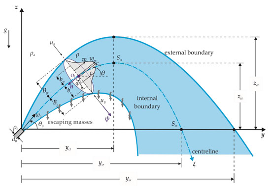
Figure 1.
Definition sketch of flow of an inclined turbulent negatively buoyant jet.
2. Materials and Methods
The escaping mass approach (EMA) model [74] is an integral model that describes the flow and mixing fields of inclined round or plane buoyant jets issuing into stationary ambient environment of uniform density. For the case of round buoyant jets, the conservation partial differential equations (PDE) of continuity, momentum and tracer have been formulated in a curvilinear cylindrical coordinate system, which is relative to the corresponding curvilinear orthogonal Cartesian coordinate system for plane buoyant jets [84]. EMA simulates the reported phenomenon ([42,47,49,50,51,52,54,60,68,69,70,71,72,73] of fluid portions that detach from the main flow of the buoyant jet, especially from the inner boundary, and move vertically upwards (or downwards for brines), causing gravitational instabilities, and consequently destroying the axial symmetry of transverse concentration and velocity profiles. EMA calculates the vertical velocity wB of the escaping masses from the buoyant jet field, employing the general definition of the local Richardson number for plume flows [9]. The concentration of these masses cB is estimated as a portion Λ of its centerline value cm. The value of Λ coefficient was adopted equal to 0.34 [74], where Λ includes the value π/4 for round buoyant jets) for all cases in the inclination range −75° ≤ θ0 ≤ −15° (or 15° ≤ θ0 ≤ 75° of negatively buoyant jets). Additionally, EMA is equipped with the second order approach (SOA), to include the variable second-order effect of turbulence to the mean flow properties [9].
EMA’s development [74] is based on PDEs of volume momentum and tracer’s conservation, concerning the Reynolds approximation for mean flow and mixing properties and their fluctuations in steady-state conditions. Additionally, the usually accepted assumptions of (a) Boussinesq’s approximation made for small initial density differences; (b) Prandtl’s boundary-layer approximation; (c) negligible molecular viscosity terms and (d) no swirl are adopted. Regarding flow symmetry with respect to the centerline ξ axis of the curvilinear coordinate system Ol(r, φ, ξ), the governing equations of the model are:
Continuity
ξ–momentum
ψ–momentum
Mass tracer
where w, u are the mean velocity components in the directions ξ and r, respectively and w′, u′ are their corresponding turbulent fluctuations; r = (n2 + ψ2)1/2 is the transverse (radial) distance; is the scale factor of the coordinate system, θ is the local inclination angle of the ξ axis, is the local mean concentration and c′ the corresponding turbulent fluctuation; ρ is the local mean fluid density; w′2, w′c′, u′c′ are the local fluxes due to turbulent fluctuations of w, u, c; τrξ is the mean turbulent shear stress; pd is the dynamic pressure; is a source term for the escaping masses from the flow field of the buoyant jet; and qr is the escaping load of masses per unit area in the r direction.
The flow field is further described when Equations (1)–(4) satisfy the following boundary conditions:
On the jet axis (r = 0)
u = 0, w = wm, c = cm, τrξ = u′c′ = qr = 0, pd = pdm
On the jet boundary (r = Bw)
where UB = −uB − wB cosθ sinφ. Based on experimental measurements, the region between the nominal half-width of a buoyant jet, b0.5, and the total half-width, Bw, is characterized by intermittencies of the velocity field (see Yannopoulos & Bloutsos 2012 [74]). Therefore, our assumption is that all this region could contribute to escaping masses. The velocity wB becomes zero at r = b0.5, while has a positive value at the boundary of the buoyant jet (r = Bw). The escaping masses from the convex boundary enter the buoyant jet and are thus swept by the main flow. However, only masses from the concave boundary manage to escape when the entrainment of the buoyant jet becomes very weak or negative. Consequently, in addition to Equation (6), on the jet boundary (r = Bw) further boundary conditions are applied:
where wB and cB are the vertical velocity and concentration of escaping masses; uB is the entrainment velocity of the inclined buoyant jet at the actual boundary Bw = d0/2 + nw bw and nw = 2−1/2 [7,8]).
u = UB, w = c = τrξ = u′c′ = 0, qr = qB sinφ, pd = pde
The main flow of the buoyant jet is assumed that remains symmetrical to the jet nξ plane. Therefore, the dimensionless mean axial velocity and concentration profiles are assumed Gaussian in the zone of established flow (ZEF):
where is the nominal width of the buoyant jet where the property reduces at the e−1 of the maximum value and is the spreading rate coefficient. Thus, stands for either the mean axial velocity w or the mean concentration c.
In the zone of flow establishment (ZFE), the EMA model incorporates the advanced integral model (AIM; [85]). Thus, the actual similarity profiles of velocity and concentration are yielded by composing the flow and mixing fields of a group of infinite vertical buoyant jets issued from closely spaced sources on the basis of flux conservation of momentum, buoyancy and kinetic energy for the mean motion and enhancing the dynamic adaptation of the individual buoyant jet axes to the group centreline.
The entrainment velocity u is calculated using the transverse velocity profile hu/wm that is produced by integrating the equation of continuity (1) with respect to distance r [9,74]:
According to [74], the vertical velocity wB of the escaping masses at the inner boundary is estimated as:
where p = 0.144, Kw = 0.11, λBp = 1.15, λp = 1.04, Rp = 0.3521 and Yp = 1.001 [74]. Additionally, the concentration cB of the escaping fluid by the inner boundary is assumed proportional to the corresponding centerline concentration as:
where Λ is a constant that is determined approximately to 0.34 [74].
3. Variation of Basic Parameters
Integration of the PDE of tracer mass (4), under the assumptions (5)–(8) yields the ordinary differential equation (ODE) of tracer mass , which gives the longitudinal variation of the slop of the buoyancy flux [74]. Figure 2 shows the variation of the normalized buoyancy flux with respect to the dimensionless distance Ξ. It is apparent that the buoyancy flux reduces along centerline path until Ξ 10 and then stabilizes to a constant value. This reduction increases via initial inclination angle θ0 until θ0 40°–45° and then decreases up to 75°. Thus, as seen in Section 4, the distance ycr increases until θ0 40°–45° and then decreases up to a minimum value approaching zero for vertical discharges.
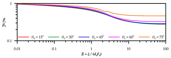
Figure 2.
Variation of the normalized buoyancy flux β/β0 with dimensionless distance Ξ = ξ/(d0F0) and initial inclination θ0.
After the flow bends over, beyond the cross section where the maximum zct occurs, the buoyancy flux becomes positive. The major part of this region is beyond Ξ 10 (Figure 2). Therefore, the stability of the buoyancy flux means that the assumption made regarding the escaping mass has no effect in the region of positive buoyancy flux.
The longitudinal variation of the local angle θ of the buoyant jet axis to horizontal with respect to the dimensionless distance Ξ = ξ/(d0F0) for various initial inclination angles θ0 (θ0 = 15°, 30°, 45°, 60°, 75°) and initial Froude numbers F0 (F0 = 5, 20) is shown in Figure 3. It is apparent that the effect of F0 to θ is rather insignificant for practical applications.
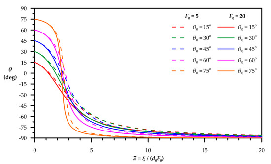
Figure 3.
Variation of local centerline angle θ to horizontal with dimensionless distance Ξ = ξ/(d0F0) and initial inclination θ0 for F0 = 5 and F0 = 20.
4. Results and Discussion
PDEs (1)–(4) are integrated with respect to r and ϕ on the actual cross-section of a round buoyant jet under the aforementioned boundary conditions, the spreading concept [9,85] and all the appropriate approximations [74]. The integration produces a system of ordinary differential equations (ODE) that is solved using a 4th order Runge-Kutta method [86]. More details about the procedure may be found at the relative paper of Yannopoulos and Bloutsos [74].
In this paper, EMA is applied to predict the mean flow geometrical quantities and mixing characteristics for inclined negatively turbulent buoyant jets for initial inclination angles 15° ≤ θ0 ≤ 75° and initial densimetric Froude numbers 4 ≤ F0 ≤ 100. For each angle, in the range 15° ≤ θ0 ≤ 75°, the variation of the non-dimensional geometric quantities of zct/d0, zet/d0, yct/d0, ycr/d0 and yer/d0 and mixing characteristics Sct and Scr are calculated for every initial Froude numbers 4 ≤ F0 ≤ 100. For every θ0, these quantities vary proportionally to the Froude number by a constant ki (among others: [49,53,54]) as:
where ki (i = 1, …, 7) is the proportionallity constant. The results are compared to experimental data available in the literature published by several researchers, as well as to other numerical models predictions such as CorJet, VisJet, the reduced buoyancy flux (RBF) model by Oliver et al. [58], modified RBF by Crowe et al. [61] and analytical solutions proposed by Kikkert et al. [49]. Available data from CFD analysis [76,78,81,82] are also used for comparisons.
Figure 4 shows the variation of dimensionless centerline terminal rise height zct to the initial inclination angle. EMA’s prediction is compared to available experimental data. The terminal rise height EMA passes through the scatter of experimental data following their trend. The latter is more obvious if a polynomial fit to experimental data [45,47,49,50,51,54,57,58,59,61,73,81,87,88] is made. For this purpose, a third degree polynomial is fitted to experimental data using the least square method. The equation of the polynomial is presented in Table 1. In the range 15° ≤ θ0 ≤ 75° EMA’s prediction is very close to the polynomial fit. It must be noted that EMA predicts the centerline as the midpoint of the round cross-section. The same procedure is followed by Bosanquet et al. [87] and Bashitialshaaer et al. [88]. Instead, Cipollina et al. [45], Kikkert et al. [49], Ferrari and Querzoli [47], Shao and Law [50], Lai and Lee [51], Oliver et al. [58], Nikiforakis et al. [89], Crowe et al. [61], Ramakanth [73], and Zhang et al. [81] determine the position of centerline as the point where the transverse profile of velocity or concentration is maximized. In particular, this point is shifted towards the external edge, moving away from the midpoint of cross-section. As the initial inclination angle is rising, the deviation of actual transverse profile is deviates intensively from the Gaussian presenting this difference, while, when the initial inclination reaches the vertical, this deviation is reduced, and EMA’s prediction coincides with the experimental data. Thus, the deviation between EMA’s prediction and the experimental data in the range 20° < θ0 < 70° is reasonably expected. In Figure 4b, EMA’s prediction of centerline terminal rise height is compared to other models results. For θ0 < 30° all models almost coincide. For θ0 > 30°, Kikkert’s analytical solution and the RBF model are diverging upwards calculating higher values than EMA’s and modified RBF’s predictions that approximately coincide up to 75°. The commercial packages CorJet and VisJet are underestimating the centerline terminal rise height for θ0 > 30°. In Figure 4b, the results of CFD analysis from Gildeh et al. [78,79] Oliver et al. [76] and Zhang et al. [81,82] for a variety of simulations are included. CFD’s results are for the most usual initial inclination angles of 15°, 30°, 45° and 60°. For 15°, all CFD’s results coincide, showing that the option of RANS or the most sophisticated LES approach does not have major effect on the results. There are significant differences among CFD simulations for θ0 = 30°, 45° and 60°, where the scatter of the results is maximized for θ0 = 45°. In any case, EMA predictions are within experimental data.
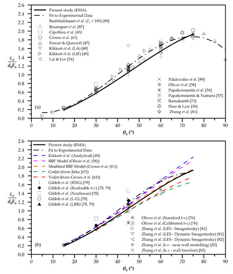
Figure 4.
Escaping mass approach’s (EMA’)s prediction of dimensionless centerline terminal height and comparison with (a) experimental data, and (b) other models’ predictions.

Table 1.
Equations of polynomial fits (3rd degree) to experimental data.
The geometric parameter of the final rising height of the external edge (boundary) zet of the dense jets is of great environmental importance, because it indicates whether the mixing processes are taking place under the water surface or not. The dimensionless values of zet that are calculated by the EMA model through the initial inclination angles are shown on Figure 5a,b. In Figure 5a, the EMA’s results are compared to previous published experimental data, and in Figure 5b, the performance of EMA is compared to other models. Again EMA, without intense deviation, follows the trend of a third degree polynomial fitted to experimental data [38,40,41,42,43,44,45,48,49,50,51,53,56,58,60,69,73,81,88,89,90,91,92,93] (Table 1). In Figure 5a, the experimental data of Nemlioglou and Roberts [48] and Bloomfield and Kerr [44] are the upper and lower data of the scatter, respectively. The wide scatter of experimental results is due to the different definitions of the external edge of the buoyant jet among the investigators. Indicatively, Kikert et al. [49] and Oliver et al. [58,78] define the external boundary at a distance twice the concentration spread, while Papakonstantis et al. [54] define this length as 1.5 times the concentration spread. Lai and Lee [51] and Abessi and Roberts [60] define the boundary at a locus where concentration values c are 25% or 10% the maximum concentration (cmax) at centerline, respectively. Similarly, Jiang et al. [52] and Zhang et al. [81] define the external boundary at c/cmax = 5% and Shao and Law [50] and Gildeh et al. [78] define the external boundary at c/cmax = 3%. According to EMA, the outer boundary of the jet is defined at a distance Bc = d0/2 + nc λ bw, where bw is the nominal spread width of the velocity field of the buoyant jet, λ is the concentration-to-velocity spreading rate coefficient ratio and nc is the non-dimensional total spread of concentrations of a buoyant that according to profile measurements by Ramaprian and Chandrasekhara [94] and Shao and Law [50] is approximately 1.9. More details can be found at the relative paper of Yannopoulos and Bloutsos [74]. Among EMA’s prediction and Kikkerts’s solution, the RBF and modified RBF models there are slight differences up to approximately 70°. A little deflection occurs between EMA’s and CorJet’s prediction for the cutoff level of c/cmax = 3%. As VisJet’s boundary is defined at 0.25 cmax, its results are like CorJet’s cutoff level of 25%, and obviously differ to the EMA relative values.
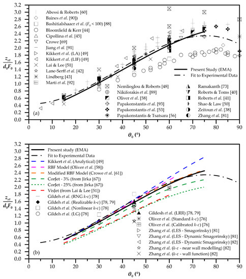
Figure 5.
EMA’s prediction of dimensionless terminal height of external edge and comparison with (a) experimental data, and (b) other models’ predictions.
In Figure 6a,b, the dimensionless horizontal distance to centerline terminal rise height yct predicted by EMA is shown. The distance yct is increasing gradually up to initial angle of 45°, approximately, and then decreases smoothly up to 75°. Similar behavior is observed at experimental data of various previous works demonstrating the good performance of EMA. Excluding the experiments of Bosanquet et al. [87] and Lindberg [43], the experimental scatter is quite narrow, and EMA predictions are within the experimental data for the range 15° ≤ θ0 ≤ 75°. CFD analyses provide data only for initial angles of 15°, 30°, 45° and 60°. The scatter of CFD data seems to be wider than experiments. Both CorJet and VisJet diverge from experimental data, underestimating the horizontal distance of centerline peak. EMA’s predictions underestimate the corresponding experimental data, following the trend of a third degree polynomial fitted to experimental data [43,45,49,50,51,53,56,58,61,73,81,87,89] (Table 1).
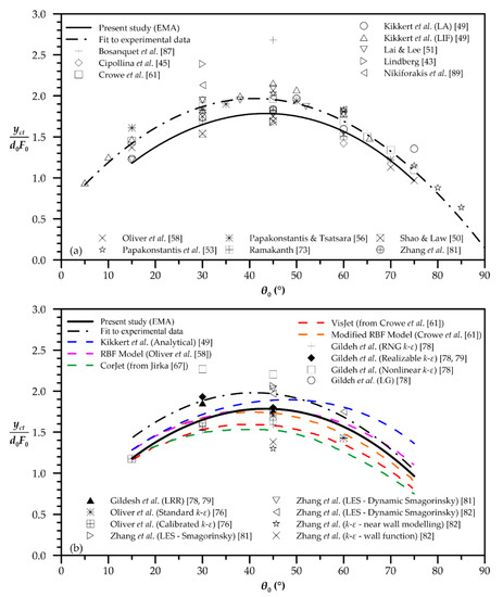
Figure 6.
EMA’s prediction of dimensionless horizontal location of centerline terminal height and comparison with (a) experimental data, and (b) other models’ predictions.
The prediction of the dimensionless horizontal location of the return point of jet axis to initial level, ycr, is shown in Figure 7. EMA’s results are compared to several experimental data for various initial inclinations in Figure 7a. Comparing EMA’s prediction to experimental fit line [41,45,47,48,49,50,51,52,54,57,58,60,61,73,81,89,91,92] (Table 1), it is obvious that EMA follows the fit line, underestimating the return point location in the whole range of 15° ≤ θ0 ≤ 75°. The difference is maximized for θ0 = 15°, decreases approaching approximately θ0 = 60° and slightly increases at θ0 = 75°. Comparing to other models and CFD predictions (Figure 7b), the EMA’s predictions seem to be better and rather satisfactory. Additionally, the corresponding variation of the external edge to initial inclination angle is presented in Figure 8. EMA’s predictions are compared to the experimental data of Bashitialshaaer et al. [88], Crowe [69], Nikiforakis et al. [89], Oliver [68], Papakonstantis et al. [53], Papakonstatis and Tsatsara [56], Ramakanth [73] and Zeitoun et al. [38], and the modified RBF Model [61]. Again, a third-degree polynomial is fitted to experimental data [38,53,56,68,69,73,88,89] (Table 1). The two models predict quite similar values. The divergence of the EMA model to the experimental fit line is less than 10% for initial angles in the range 15° ≤ θ0 ≤ 75°.
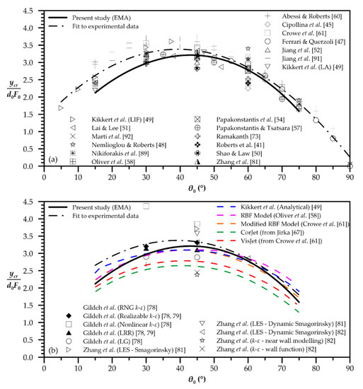
Figure 7.
EMA’s prediction of dimensionless horizontal location of centerline terminal height and comparison with (a) experimental data, and (b) other models’ predictions.
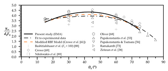
Figure 8.
EMA’s prediction of dimensionless horizontal location of external edge return point and comparison with experimental data.
Figure 9 presents the prediction of the EMA model for axial dilutions at the centerline terminal height (Sct). The prediction is compared to available experimental data. EMA’s dilution values are overestimated, compared to a third degree polynomial fit [38,40,42,50,51,54,57,58,73,81,91] (Table 1) to experimental data, in the range of initial inclination angles 15° ≤ θ0 ≤ 65°. In the range 65° < θ0 ≤ 75°, the maximum underestimation is 24.0%, which occurred for θ0 = 75°.
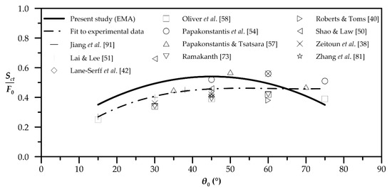
Figure 9.
EMA’s prediction of axial dilution at centerline terminal height and comparison with experimental data.
The variation of EMA’s axial dilutions at the return point (Scr) for initial inclination angles in the range 15° ≤ θ0 ≤ 75° is presented in Figure 10. Figure 10a shows the predicted EMA’s dilutions compared to available experimental data. A third degree polynomial is fitted to experimental data [40,41,48,50,51,52,54,57,59,60,73,81,91,92] (Table 1). EMA’s predictions perform a continuous increment, slightly underestimating dilution values in the range of 15° ≤ θ0 ≤ 65°, while the maximum overestimation is 12.6% for initial inclination angles greater than 65°. Comparing to other model predictions (Figure 10b), it is obvious that EMA has the better overall performance. CFD analysis by Gildesh et al. [78,79] for θ0 = 30° gave similar values approximating experimental data.
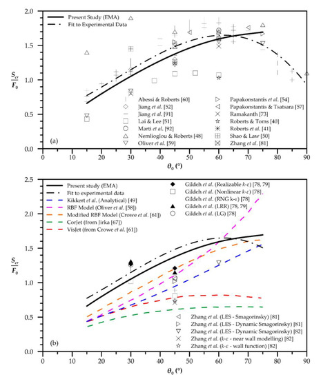
Figure 10.
EMA’s prediction of axial dilution at centerline return point and comparison with (a) experimental data, and (b) other models’ predictions.
The dimensionless path length of the centerline up to terminal height sct (Figure 11) almost coincides to corresponding experimental data of Crowe [69], Oliver [68] and Ramakanth [73], where the scatter of experimental data is negligible.
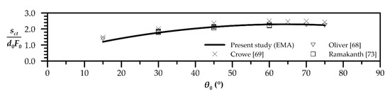
Figure 11.
EMA’s prediction of dimensionless centerline length to terminal height and comparison with experimental data.
The only existing experimental data of the path length of external edge of negatively buoyant plumes until the return point are provided by Christodoulou and Papakonstantis [95], and are compared to the corresponding predictions of EMA model in Figure 12. It is obvious that the EMA and experimental results almost coincide.
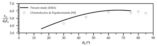
Figure 12.
EMA’s prediction of dimensionless external edge length to return point and comparison with experimental data.
5. Conclusions
A second order Gaussian integral model that incorporates the mechanism of escaping masses from an inclined buoyant jet (EMA) was applied to predict the mean flow and mixing properties of inclined turbulent negatively round buoyant jets in stationary and uniform ambient. The predictions were made for a range of initial inclination angle from 15° to 75° to the horizontal and initial Froude number from 4 to 100. EMA’s dimensionless results were compared to experimental data and other integral or numerical predictions available in the literature. For comparison reasons, a third degree polynomial is fitted to experimental data for every parameter under study. EMA’s prediction of dimensionless terminal height of external edge almost coincides to the experimental fit, while the corresponding prediction of centerline terminal height differs slightly from the polynomial fit, for initial angles θ0 from 35° to 40°. This difference is attributed to the way that centerline is defined by each researcher. EMA’s predictions of horizontal distance of centerline terminal height are lower than the experimental fit polynomial, but within the range of experimental values. Regarding the horizontal location of return point of centerline and external edge, EMA’s predictions follow the corresponding polynomial fits presenting a slight difference for the case of centerline variation. As an overall observation, EMA’s predictions agree well to the experimental data, which assures that EMA performs better than other models. The definition of buoyant jet’s centerline affects the estimated variation of axial dilution at centerline terminal height regarding the available experimental data, leading to overestimations for initial inclinations less than 45°. Additionally, EMA’s prediction of the axial dilution values at centerline return point is rather conservative compared to the corresponding experimental fit, but much closer than other models’ predictions. Finally, EMA’s of centerline length to terminal height and external edge length to return point coincides excellently to available experimental data. Overall, it seems that the application of EMA model gives reliable predictions without heavy computational cost or adopting controversial assumptions.
Author Contributions
Investigation, A.A.B. and P.C.Y.; Methodology, A.A.B. and P.C.Y.; Project administration, P.C.Y.; Software, A.A.B. and P.C.Y.; Supervision, P.C.Y.; Validation, A.A.B.; Writing–original draft, A.A.B.; Writing–review & editing, P.C.Y. All authors have read and agreed to the published version of the manuscript.
Funding
This research received no external funding.
Acknowledgments
The authors acknowledge the three reviewers’ comments that improved the paper significantly.
Conflicts of Interest
The authors declare no conflict of interest.
References
- Abraham, G. Jet diffusion in stagnant ambient fluid 1963 (Vol. Tech. Rep. 29). Delft. Available online: https://resolver.tudelft.nl/uuid:6ad300a4-94d9-44f7-9b1a-787d010d2844 (accessed on 1 July 2020).
- Fischer, B.H.; List, J.E.; Koh, R.C.; Imberger, J.; Brooks, N.H. Mixing in Inland and Coastal Waters; Academic Press, Inc.: New York, NY, USA, 1979. [Google Scholar] [CrossRef]
- Hanna, S.R.; Briggs, G.A.; Hosker, R.P. Handbook on Atmospheric Diffusion; U.S. Department of Energy: Washington, DC, USA, 1982. [CrossRef]
- Pasquill, F.; Smith, F.B. Atmospheric Diffusion, 3rd ed.; John Wiley and Sons: Chichester, UK, 1983. [Google Scholar] [CrossRef]
- Papanicolaou, P.N.; List, J.E. Investigations of round vertical turbulent buoyant jets. J. Fluid Mech. 1988, 195, 341–391. [Google Scholar] [CrossRef]
- Wang, H.; Law, A.W.-K. Second-order integral model for a round turbulent buoyant jet. J. Fluid Mech. 2002, 459, 397–428. [Google Scholar] [CrossRef]
- Jirka, G.H. Integral model for turbulent buoyant jets in unbounded stratified flows. Part I: Single Round Jet. Environ. Fluid Mech. 2004, 4, 1–56. [Google Scholar] [CrossRef]
- Lee, J.H.-W.; Chu, V. Turbulent Jets and Plumes. A Lagrangian Approach; Springer US: New York, NY, USA, 2003. [Google Scholar] [CrossRef]
- Yannopoulos, P.C. An improved integral model for plane and round turbulent buoyant jets. J. Fluid Mech. 2006, 547, 267–296. [Google Scholar] [CrossRef]
- Britter, R.E. Atmospheric dispersion of dense gases. Annu. Rev. Fluid Mech. 1989, 21, 317–344. [Google Scholar] [CrossRef]
- Ohba, R.; Kouchi, A.; Vieillard, V.; Nedelka, D. Validation of heavy and light gas dispersion models for the safetyanalysis of LNG tank. J. Loss Prev. Process. Ind. 2004, 17, 325–337. [Google Scholar] [CrossRef]
- Bellasio, R.; Bianconi, R. Online simulation system for industrial accidents. Environ. Model. Softw. 2005, 20, 329–342. [Google Scholar] [CrossRef]
- Liu, D.; Wei, J. Modelling and simulation of continuous dense gas leakage for emergency response application. J. Loss Prev. Process. Ind. 2017, 48, 14–20. [Google Scholar] [CrossRef]
- Sklavounos, S.; Rigas, F. Validation of turbulence models in heavy gas dispersion over obstacles. J. Hazard. Mater. 2004, 108, 9–20. [Google Scholar] [CrossRef]
- Gavelli, F.; Bullister, E.; Kytomaa, H. Application of CFD (Fluent) to LNG spills into geometrically complex environments. J. Hazard. Mater. 2008, 159, 158–168. [Google Scholar] [CrossRef]
- Tominaga, Y.; Stathopoulos, T. CFD simulations of near-field pollutant dispersion with different plume buoyancies. Build. Environ. 2018, 131, 128–139. [Google Scholar] [CrossRef]
- Mezher, T.; Fath, H.; Abbas, Z.; Khaled, A. Techno-economic assessment and environmental impacts of desalination technologies. Desalination 2011, 266, 263–273. [Google Scholar] [CrossRef]
- Petersen, K.L.; Paytan, A.; Rahav, E.; Levy, O.; Silverman, J.; Barzel, O.; Bar-Zeev, E. Impact of brine and antiscalants on reef-building corals in the Gulf of Aqaba—Potential effects from desalination plants. Water Res. 2018, 144, 183–191. [Google Scholar] [CrossRef] [PubMed]
- Petersen, K.L.; Frank, H.; Paytan, A.; Bar-Zeev, E. Impacts of seawater desalination on coastal environment. In Sustainable Desalination Handbook. Plant Selection, Design and Implementation; Gude, V.G., Ed.; Butterworth—Heinemann: Oxford, UK, 2018; pp. 437–464. [Google Scholar] [CrossRef]
- Lattemann, S.; Höpner, T. Environmental impact and impact assessment. Desalination 2008, 220, 1–15. [Google Scholar] [CrossRef]
- Drami, D.; Yacobi, Y.Z.; Stambler, N.; Kress, N. Seawater quality and microbial communities at a desalination plant marine outfall. A field study at the Israeli Mediterranean coast. Water Res. 2011, 45, 5449–5462. [Google Scholar] [CrossRef]
- Lin, Y.-C.; Chang-Chien, G.-P.; Chiang, P.-C.; Chen, W.-H.; Lin, Y.-C. Potential impacts of discharges from seawater reverse osmosis on Taiwan marine environment. Desalination 2013, 322, 84–93. [Google Scholar] [CrossRef]
- Frank, H.; Rahav, E.; Bar-Zeev, E. Short-term effects of SWRO desalination brine on benthic heterotrophic microbial communities. Desalination 2017, 417, 52–59. [Google Scholar] [CrossRef]
- Cambridge, M.L.; Zavala-Perez, A.; Cawthray, G.R.; Mondon, J.; Kendrick, G.A. Effects of high salinity from desalination brine on growth, photosynthesis, water relations and osmolyte concentrations of seagrass Posidonia australis. Mar. Pollut. Bull. 2017, 115, 252–260. [Google Scholar] [CrossRef]
- Cambridge, M.L.; Zavala-Perez, A.; Cawthray, G.R.; Statton, J.; Mondon, J.; Gary, K.A. Effects of desalination brine and seawater with the same elevated salinity on growth, physiology and seedling development of the seagrass Posidonia australis. Mar. Pollut. Bull. 2019, 140, 462–471. [Google Scholar] [CrossRef]
- Roberts, D.A.; Johnston, E.L.; Knott, N.A. Impacts of desalination plant discharges on the marine environment. A critical review of published studies. Water Res. 2010, 44, 5117–5128. [Google Scholar] [CrossRef]
- Missimer, T.M.; Maliva, R.G. Environmental issues in seawater reverse osmosis desalination: Intakes and outfalls. Desalination 2018, 434, 198–215. [Google Scholar] [CrossRef]
- Frank, H.; Fussmann, K.E.; Rahav, E.; Zeev, E.B. Chronic effects of brine discharge form large-scale seawater reverse osmosis. Water Res. 2019, 151, 478–487. [Google Scholar] [CrossRef] [PubMed]
- Jones, E.; Qadir, M.; van Vliet, M.T.H.; Smakhtin, V.; Kang, S.-M. The state of desalination and brine production. A global outlook. Sci. Total Environ. 2019, 657, 1343–1356. [Google Scholar] [CrossRef] [PubMed]
- Voutchkov, N. Overview of seawater concentrate disposal alternatives. Desalination 2011, 273, 205–219. [Google Scholar] [CrossRef]
- Shrivastava, I.; Adams, E.E. Pre-dilution of desalination reject brine: Impact on outfall dilution in. J. Hydro-Environ. Res. 2019, 24, 28–35. [Google Scholar] [CrossRef]
- Turner, J. Jets and plumes with negative or reversing buoyancy. J. Fluid Mech. 1966, 26, 779–792. [Google Scholar] [CrossRef]
- Abraham, G. Jets with Negative Buoyancy in Homogeneous Fluid. J. Hydraul. Res. 1967, 5, 235–248. [Google Scholar] [CrossRef]
- Bloomfield, L.J.; Kerr, R.C. A theoretical model of a turbulent fountain. J. Fluid Mech. 2000, 424, 197–216. [Google Scholar] [CrossRef]
- Kaminski, E.; Tait, S.; Carazzo, G. Turbulent entrainment in jets with arbitrary buoyancy. J. Fluid Mech. 2005, 526, 361–376. [Google Scholar] [CrossRef]
- Baddour, R.E.; Zhang, H. Density Effect on Round Turbulent Hypersaline Fountain. J. Hydraul. Eng. 2009, 135, 57–59. [Google Scholar] [CrossRef]
- Ahmad, N.; Baddour, R.E. A review of sources, effects, disposal methods, and regulations of brine into marine environments. Ocean Coast. Manag. 2014, 87, 1–7. [Google Scholar] [CrossRef]
- Zeitoun, M.A.; Mcllhenny, W.F.; Reid, R.O.; Wong, C.-M.; Savage, W.F.; Rinne, W.W.; Gransee, C.L. Conceptual Designs of Outfall Systems for Desalting Plants; Report No. 550; United States Department of the Interior: Washington, DC, USA, 1970.
- Pincince, A.B.; List, E.J. Disposal of brine into an estuary. J. Water Pollut. Control Fed. 1973, 45, 2335–2344. [Google Scholar]
- Roberts, P.J.; Toms, G. Inclined dense jets in flowing current. J. Hydraul. Eng. 1987, 113, 323–341. [Google Scholar] [CrossRef]
- Roberts, P.J.; Ferrier, A.; Daviero, G. Mixing in Inclined Dense Jets. J. Hydraul. Eng. 1997, 123, 693–699. [Google Scholar] [CrossRef]
- Lane-Serff, G.F.; Linden, P.F.; Hillel, M. Forced, angled plumes. J. Hazard. Mater. 1993, 33, 75–99. [Google Scholar] [CrossRef]
- Lindberg, W.R. Experiments on negatively buoyant jets, with and without cross-flow. In Recent Research Advances in the Fluid Mechanics of Turbulent Jets and Plumes; NATO Science Series; Davies, P.A., Valente Neves, M.J., Eds.; Kluwer Academic Publishers: Dordrecht, The Netherlands, 2012; pp. 131–145. [Google Scholar]
- Bloomfield, L.J.; Kerr, R.C. Inclined turbulent fountains. J. Fluid Mech. 2002, 451, 283–294. [Google Scholar] [CrossRef]
- Cipollina, A.; Brucato, A.; Grisafi, F.; Nicosia, S. Bench-Scale Investigation of Inclined Dense Jets. J. Hydraul. Eng. 2005, 131, 1017–1022. [Google Scholar] [CrossRef]
- Ferrari, S.; Querzoli, G. Sea discharge of brine from desalination plants a laboratory model of negatively buoyant jets. In Proceedings of the MWWD 2004-3rd International Conference on Marine Waste Water Discharges and Marine, Catania, Italy, 27 September–2 October 2004. [Google Scholar]
- Ferrari, S.; Querzoli, G. Mixing and re-entrainment in a negatively buoyant jet. J. Hydraul. Res. 2010, 48, 632–640. [Google Scholar] [CrossRef]
- Nemlioglu, S.; Roberts, P.J. Experiments on Dense Jets Using Three-Dimensional Laser-Induced Fluorescence (3DLIF). In Proceedings of the 4th International Conference on Marine Wastewater Disposal and Marine Environment (MWWD), Antalya, Turkey, 6–10 November 2006. [Google Scholar]
- Kikkert, G.A.; Davidson, M.J.; Nokes, R.I. Inclined Negatively Buoyant Discharges. J. Hydraul. Eng. 2007, 133, 545–554. [Google Scholar] [CrossRef]
- Shao, D.; Law, A.W.-K. Mixing and boundary interactions of 30° and 45° inclined dense jets. Environ. Fluid Mech. 2010, 10, 521–533. [Google Scholar] [CrossRef]
- Lai, C.C.-K.; Lee, J.H.-W. Mixing of inclined dense jets in stationary ambient. J. Hydro-Environ. Res. 2012, 6, 9–28. [Google Scholar] [CrossRef]
- Jiang, B.; Law, A.W.-K.; Lee, J.H.-W. Mixing of 30° and 45° Inclined Dense Jets in Shallow Coastal Waters. J. Hydraul. Eng. 2014, 140, 241. [Google Scholar] [CrossRef]
- Papakonstantis, I.G.; Christodoulou, G.C.; Papanicolaou, P.N. Inclined negatively buoyant jets 1: Geometrical characteristics. J. Hydraul. Res. 2011, 49, 3–12. [Google Scholar] [CrossRef]
- Papakonstantis, I.G.; Christodoulou, G.C.; Papanicolaou, P.N. Inclined negatively buoyant jets 2: Concentration measurements. J. Hydraul. Res. 2011, 49, 13–22. [Google Scholar] [CrossRef]
- Nikiforakis, I.K.; Stamou, A.I.; Christodoulou, G.C. A modified integral model for negatively buoyant jets in a stationary ambient. Environ. Fluid Mech. 2015, 15, 939–957. [Google Scholar] [CrossRef]
- Papakonstantis, I.G.; Tsatsara, E.I. Trajectory characteristics of inclined turbulent dense jets. Environ. Process. 2018, 5, 539–554. [Google Scholar] [CrossRef]
- Papakonstantis, I.G.; Tsatsara, E.I. Mixing characteristics of inclined turbulent dense jets. Environ. Process. 2019, 6, 525–541. [Google Scholar] [CrossRef]
- Oliver, C.J.; Davidson, M.J.; Nokes, R.I. Predicting the near-field mixing of desalination discharges in a stationary environment. Desalination 2013, 309, 148–155. [Google Scholar] [CrossRef]
- Oliver, C.J.; Davidson, M.J.; Nokes, R.I. Removing the boundary influence on negatively buoyant jets. Environ. Fluid Mech. 2013, 13, 625–648. [Google Scholar] [CrossRef]
- Abessi, O.; Roberts, P.J. Effect of nozzle orientation on dense jets in stagnant environments. J. Hydraul. Eng. 2015, 141. [Google Scholar] [CrossRef]
- Crowe, A.T.; Davidson, M.J.; Nokes, R.I. Modified reduced buoyancy flux model for desalination discharges. Desalination 2016, 378, 53–59. [Google Scholar] [CrossRef]
- Crowe, A.T.; Davidson, M.J.; Nokes, R.I. Velocity measurements in inclined negatively buoyant jets. Environ. Fluid Mech. 2016, 16, 503–520. [Google Scholar] [CrossRef]
- Wood, I.R.; Bell, R.G.; Wilkinson, D.L. Ocean Disposal of Wastewater; Advanced series on ocean engineering; World Scientific: Singapore, 1993; Volume 8. [Google Scholar] [CrossRef]
- Morton, B.R.; Taylor, G.I.; Turner, J.S. Turbulent gravitational convection from maintained and instantaneous sources. Proc. R. Soc. A 1956, 234, 1196. [Google Scholar] [CrossRef]
- Papanicolaou, P.N.; Papakonstantis, I.G.; Christodoulou, G.C. On the entrainment coefficient in negatively buoyant jets. J. Fluid Mech. 2008, 614, 447–470. [Google Scholar] [CrossRef]
- Lee, J.H.; Cheung, V. Generalized Lagrangian Model for Buoyant Jets in Current. J. Environ. Eng. 1990, 116, 1085–1106. [Google Scholar] [CrossRef]
- Jirka, G.H. Improved Discharge Configurations for Brine Effluents from Desalination Plants. J. Hydraul. Eng. 2008, 134, 116–120. [Google Scholar] [CrossRef]
- Oliver, C.J. Near Field Mixing of Negatively Buoyant Jets. Ph.D. Thesis, Department of Civil and Natural Resources Engineering, University of Canterbury, Christchurch, New Zealand, 2012. [Google Scholar]
- Crowe, A.T. Inclined Negatively Buoyant Jets and Boundary Interaction. Ph.D. Thesis, Department of Civil and Natural Resources Engineering, University of Canterbury, Christchurch, New Zealand, 2013. [Google Scholar]
- Besalduch, L.A.; Badas, M.G.; Ferrari, S.; Querzoli, G. Experimental studies for the characterization of the mixing processes in negative buoyant jets. EPJ Web Conf. 2013, 45. [Google Scholar] [CrossRef]
- Besalduch, L.A.; Badas, M.G.; Ferrari, S.; Querzoli, G. On the near field behavior of inclined negatively buoyant jets. EPJ Web Conf. 2014, 67, 2007. [Google Scholar] [CrossRef]
- Jiang, M.; Law, A.W.-K.; Lai, A.C. Turbulence characteristics of 45° inclined dense jets. Environ. Fluid Mech. 2019, 19, 27–54. [Google Scholar] [CrossRef]
- Ramakanth, A. Quantifying Boundary Interaction of Negatively Buoyant Jets. Ph.D. Thesis, Department of Civil and Natural Resources Engineering, University of Canterbury, Christchurch, New Zealand, 2016. [Google Scholar]
- Yannopoulos, P.C.; Bloutsos, A.A. Escaping mass approach for inclined plane and round buoyant jets. J. Fluid Mech. 2012, 695, 81–111. [Google Scholar] [CrossRef]
- Vafeiadou, P.; Papakonstantis, I.; Christodoulou, G. Numerical simulation of inclined negatively buoyant jets. In Proceedings of the 9th International Conference on Environmental Science and Technology, Rhodes, Greece, 1–3 September 2005. [Google Scholar]
- Oliver, C.J.; Davidson, M.J.; Nokes, R.I. k-ε Predictions of the initial mixing of desalination discharges. Environ. Fluid Mech. 2008, 8, 617–625. [Google Scholar] [CrossRef]
- Gildeh, H.K.; Mohammadian, A.; Nistor, I.; Qiblawey, H. Numerical Modeling of Turbulent Buoyant Wall Jets in Stationary Ambient Water. J. Hydraul. Eng. 2014, 140. [Google Scholar] [CrossRef]
- Gildeh, H.K.; Mohammadian, A.; Nistor, I.; Qiblawey, H. Numerical modeling of 30° and 45° inclined dense turbulent jets in stationary ambient. Environ. Fluid Mech. 2015, 15, 537–562. [Google Scholar] [CrossRef]
- Gildeh, H.K.; Mohammadian, A.; Nistor, I.; Qiblawey, H.; Yan, X. CFD modeling and analysis of the behavior of 30° and 45° inclined dense jets—New numerical insights. J. Appl. Water Eng. Res. 2016, 4, 112–127. [Google Scholar] [CrossRef]
- Ardalan, H.; Vafaei, F. CFD and Experimental Study of 45° Inclined Thermal-Saline Reversible Buoyant Jets in Stationary Ambient. Environ. Process. 2019, 6, 219–239. [Google Scholar] [CrossRef]
- Zhang, S.; Jiang, B.; Law, A.W.-K.; Zhao, B. Large eddy simulations of 45° inclined dense jets. Environ. Fluid Mech. 2016, 16, 101–121. [Google Scholar] [CrossRef]
- Zhang, S.; Law, A.W.-K.; Jiang, M. Large eddy simulations of 45° and 60° inclined dense jets with bottom. J. Hydro-Environ. Res. 2017, 15, 54–66. [Google Scholar] [CrossRef]
- Cintolesi, C.; Petronio, A.; Armenio, V. Turbulent structures of buoyant jet in cross-flow studied through large-eddy simulation. Environ. Fluid Mech. 2019, 19, 401–433. [Google Scholar] [CrossRef]
- Bloutsos, A.A.; Yannopoulos, P.C. Curvilinear Coordinate System for Mathematical Analysis of Inclined Buoyant Jets Using the Integral Method. Math. Probl. Eng. 2018, 2018. [Google Scholar] [CrossRef]
- Yannopoulos, P.C. Advanced integral model for groups of interacting round turbulent buoyant jets. Environ. Fluid Mech. 2010, 10, 415–450. [Google Scholar] [CrossRef]
- Kreyszig, E. Advanced Engineering Mathematics, 10th ed.; John Wiley & Sons, Inc.: Hoboken, NJ, USA, 2011. [Google Scholar]
- Bosanquet, C.H.; Horn, G.; Thring, M.W.; Taylor, G.I. The effect of density differences on the path of jets. Proc. R. Soc. A 1961, 263, 340–352. [Google Scholar] [CrossRef]
- Bashitialshaaer, R.; Larson, M.; Persson, K.M. An Experimental Investigation on Inclined Negatively Buoyant Jets. Water 2012, 2012, 720–738. [Google Scholar] [CrossRef]
- Nikiforakis, I.K.; Christodoulou, G.C.; Stamou, A.I. Bottom concentration field due to impingement of inclined dense jet on a slope. In Proceedings of the 7th International Symposium of Environmental Hydraulics, Singapore, 7–8 January 2014. [Google Scholar]
- Baines, W.; Turner, J.; Campbell, I. Turbulent fountains in an open chamber. J. Fluid Mech. 1990, 212, 557–592. [Google Scholar] [CrossRef]
- Jiang, M.; Law, A.W.-K.; Song, J. Mixing characteristics of inclined dense jets with different nozzle geometries. J. Hydro-Environ. Res. 2019, 27, 116–128. [Google Scholar] [CrossRef]
- Marti, C.L.; Antenucci, J.P.; Luketina, D.; Okely, P.; Imberger, J. Near-Field Dilution Characteristics of a Negatively Buoyant Hypersaline Jet Generated by a Desalination Plant. J. Hydraul. Eng. 2011, 137, 57–65. [Google Scholar] [CrossRef]
- Papakonstantis, I.; Kampourelli, M.; Christodoulou, G. Height of rise of inclined and vertical negatively buoyant. In Proceedings of the 32nd IAHR Congress, Venice, Italy, 1–6 July 2007. [Google Scholar]
- Ramaprian, R.B.; Chandrasekhara, M. Study of Vertical Plane Turbulent Jets and Plumes; Tech. Rep. IIHR No. 257; Iowa Institute of Hydraulic Research, University of Iowa: Iowa City, IA, USA, 1983. [Google Scholar]
- Christodoulou, G.C.; Papakonstantis, I.G. Simplified estimates of trajectory of inclined negatively buoyant jets. In Environmental Hydraulics, Proceedings of the 6th International Symposium on Environmental Hydraulics, Athens, Greece, 23–25 June 2005; Christodoulou, G.C., Stamou, A.I., Eds.; Taylor and Francis Group: London, UK, 2010. [Google Scholar]
© 2020 by the authors. Licensee MDPI, Basel, Switzerland. This article is an open access article distributed under the terms and conditions of the Creative Commons Attribution (CC BY) license (http://creativecommons.org/licenses/by/4.0/).