Abstract
We have conducted experiments of the Faraday instability in a network of square cells filled with water for driving frequencies and amplitudes in the intervals Hz and mm, respectively. The experiments were aimed at studying the effects of varying the size of the cells on the surface wave patterns. Images of the surface wave patterns were recorded with a high-speed camera. The time series of photographs composing each video was Fourier analyzed, and information about the waveforms was obtained by using a Pearson correlation analysis. For small square cells of side length cm, adjacent cells collaborate synchronously to form regular patterns of liquid bumps over the entire grid, while ordered matrices of oscillons are formed at higher frequencies. As the size of the cells is increased to cm, collective cell behaviour at lower frequencies is no longer observed. As the frequency is increased, a transition from three triangularly arranged oscillons within each cell to three, or even four, irregularly arranged oscillons is observed. The wave patterns, the waveforms and the energy content necessary to excite Faraday waves are seen to depend on the cell size.
1. Introduction
When a container that is partially filled with a liquid is subjected to vertical vibrations, a pattern of standing waves is generally observed on the surface of the liquid. These waves are known as Faraday waves. In 1831, Faraday [1] reported for the first time that the frequency of the vibrations on the liquid surface are sub-harmonic because they oscillate at half of the harmonic excitation frequency. This idea was later challenged by Mathiessen [2,3], who found experimentally that the vibrations were synchronous. This disagreement, between Faraday and Matthiessen, led Lord Rayleigh to conduct his own experiments [4], finding in two different ways that their results agreed with Faraday’s statement. He also identified these oscillations as parametric instabilities and suggested that his theory [5] can be extended to explain Faraday’s experiment. It wasn’t until 1954 that Benjamin and Ursell [6] using linear theory confirmed the sub-harmonic nature of the instability.
In the last century, efforts have been made to extend Benjamin and Ursell’s analysis to finite amplitudes by incorporating weak nonlinearities. However, most of these studies gave rise to controversies. For instance, Dodge et al. [7], Henstock and Sani [8], and Meron and Procaccia [9] performed analyses for finite amplitudes, whose results have been questioned by Miles [10]. Ockendon and Ockendon [11] extended Benjamin and Ursell’s analysis to small, finite amplitudes, but without explicitly calculating the interaction parameter that measures the nonlinear inertial effects. They also determined the bifurcation structure of the evolution equations, including the qualitative effects of linear damping. On the other hand, Miles [10] calculated the interaction parameter and incorporated the effects of linear damping. Moreover, Gu et al. [12] calculated the interaction parameter for a rectangular cylinder, while Virnig et al. [13] were able to measure the wave amplitudes at steady-state conditions in large rectangular cylinders in which the viscous and the capillary effects were small, obtaining results in good agreement with the calculations of Gu et al. [12].
With the growing interest in nonlinear dynamics and temporal chaos, experiments on Faraday waves have gained considerable attention. For example, Keolian et al. [14] observed a chaotic state in a strongly driven circular container, while Gollub and Meyer [15] studied the transition to chaos of a single oscillation mode in a circular cell. Later on, Ciliberto and Gollub [16,17] showed how the effects of two superimposed modes can lead to chaos, and Simonelli and Gollub [18] studied the interactions in two modes that were almost degenerate by symmetry.
From a suitable choice of experimental parameters, several different patterns can be observed, consisting of a set of ordered geometrical figures such as lines, squares, triangles, and hexagons. Kudrolli et al. [19] reported superlattice patterns, while Arbell and Fineberg [20,21] observed local structures using two-frequency forcings. Understanding the types of patterns that form is challenging. The instability threshold and observed patterns depend on the viscosity and surface tension of the fluid, the dimensionless acceleration, , of the formation, the shape and the size of the container. Furthermore, fluctuations in the frequency and amplitude of the exciting force may drive a defined pattern to change into a mixed state with a fraction of space-time chaos [22]. On the other hand, the mechanisms of pattern selection have been investigated by Silber et al. [23] and Skeldon and Guidoboni [24], using the tools of symmetry and bifurcation theory. Numerical simulations, involving the solution of the Navier–Stokes equations coupled to a frontal tracking method for treatment of the free surface, have also started to appear by assuming that the liquid surface is perfectly flat at the edge of the side walls [25,26]. However, such simulations do not reproduce actual experiments where the dynamics of the meniscus is important [27]. In particular, for small containers, there is a strong coupling between the capillary waves generated by the meniscus and the Faraday waves [28].
An interesting variant of the Faraday experiment was carried out by Delon et al. [29], who have divided the free surface of the liquid into an array of square cells. They performed a frequency sweep from 10 to 16 Hz and observed how liquid peaks formed synchronously at the vertices of the cells as a result of the collective behaviour of the liquid contained in the cells. More recently, Peña-Polo et al. [30] conducted similar experiments for square cell networks in the frequency range between 10 and 28 Hz. They observed the formation of regular patterns over the network consisting of liquid bumps at the cell vertices for Hz, while at Hz a mixed state was observed consisting of localized oscillons at the cell centres in one part of the network and regular bumps at the cell vertices in the other part. At frequencies in the range Hz, localized oscillons at the cell centres were always observed and, at even higher frequencies ( Hz), disordered patterns appeared, which corresponded to periodic harmonic waves. They also assessed that the surface oscillation frequencies for Hz were all sub-harmonic.
Here, we perform similar experiments to those of Peña-Polo et al. [30] by varying the size of the square cells. The effects of varying the size of the square cells on the surface wave patterns are studied for a fine sweep of the amplitudes and frequencies of the driving force. For driving frequencies in the range Hz, we provide a quantitative picture of the parametrically excited waves from a Fourier and a Pearson correlation analysis to determine their power spectra and waveforms. The results show that the wave patterns, the waveforms and the energy content required exciting Faraday waves in a cell network depending on the cell size.
2. Experimental Setup and Methods
The experimental setup consists of a transparent acrylic container with a horizontal square base of size cm and height 8 cm fixed rigidly to a TIRA TV51075 stirrer. This device can deliver a maximum force of 75 N with a peak-to-peak amplitude oscillation of 1 cm. Two different styrene square cell networks are employed differing in the cell size. One network is composed of 81 square cells of sides cm and the other of 25 square cells of sides cm. In both cases, the cells have a height cm and the networks are fixed to the bottom of the acrylic vessel. The cells are filled with distilled water doped with methylene blue up to a depth of cm. With these parameters, the total payload was 1.6 kg and the maximum allowed dimensionless peak-to-peak acceleration was 4.55. In order to ensure the same level of liquid over the entire network, each cell was provided with a circular hole of diameter 0.5 mm at the bottom.
A control software provided by the manufacturer is used to drive the shaker from which an input value of the amplitude, A, and frequency, F, is supplied manually. The input frequency is received by a VR-8500 controller connected to a host computer, which produces a sinusoidal signal as output. A piezoelectric accelerometer magnetically attached to the oscillation platform and connected to the VR8500 controller is employed to measure the amplitude of the forcing oscillation. The output signals are amplified by a Tira BAA120 power amplifier connected to the shaker. The amplitude and frequency of the produced signals are checked by a multifunctional data acquisition board and processed by the host computer, where a software is run to provide the oscillation amplitude in millimeters and the frequency in Hz.
A REDLAKE MotionXTRA HG-100K camera (DEL Imaging Systems, LLC, Woodsville, NH, USA) was used to capture images at high speed, which was placed over the assembly at a height of 80 cm. Images were captured at a resolution of pixels at a speed of 2016 fps and an exposure time of 250 s. The integration time of the images (=2.99 s) was kept well below half the wave period so that the images can be considered to be instantaneous photographs of the surface. The illumination was provided by a square array of four white light lamps with a color temperature of 6500 K each, which produced more than 22,000 lumens of visible light. These lamps were mounted symmetrically at a height of 20 cm from the surface of the fluid. In order to avoid alteration of the fluid properties, the lamps were turned on only during video recording for no more than about 10 s. These images were then processed and stored in a dedicated digital image system.
In this work, we consider the variation of the forcing frequency and amplitude within the intervals Hz and mm, respectively. The dots in Figure 1 mark the locus in the -plane of the experimental tests. The minimum frequency Hz was chosen based on the fact that, for lower values of F, the wavelengths of the corresponding perturbations will be larger than the size of the smaller cells ( cm) and so no excitation of the liquid surface will take place. For these cells, the diagonal is ≈3.53 cm, which is comparable to the wavelength of the forcing oscillations for Hz. Therefore, for frequencies above this threshold, after a transient state, adjacent cells synchronize to form regular patterns over the entire grid [29,30]. Cells of size cm will have a larger diagonal (≈7.07 cm) and therefore excitation of the liquid surface will indeed occur for frequencies lower than 10 Hz. However, for the sake of measuring the effects of varying the size of the cell on the resulting wave patterns, we have considered the same frequency and amplitude ranges for both sequences of experiments. This was possible because the payload was the same for both grids. In order to keep the shaker below 60% of its stroke capability, the maximum amplitudes were limited to 3 mm for Hz, while, at frequencies of 22 Hz, it was necessary to reduce the amplitudes to less than about 2.5 mm. Each experiment represented by a dot in Figure 1 was repeated up to five times to assess the reproducibility of the observed patterns for given amplitude and frequency of the forcing.
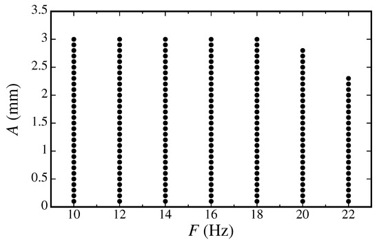
Figure 1.
The dots represent the locus in the -plane of the experimental tests. The same forcing frequencies and amplitudes are used for both types of cell networks.
An analysis of the fluid surface behaviour was performed by processing the videos of all experiments by means of a Pearson correlation of the time series of photographs composing each video. A fast Fourier transform (FTT) of each photographic image is computed and a correlation coefficient as a function of time is obtained by comparing each successive image in the time series with the initial one. The two-dimensional correlation coefficients obtained this way provide a measure of the difference between the first image and all successive images contained in the video. The output of the FTT gives information of each image in the frequency domain, where each point represents a particular frequency contained in the actual image. In other words, it represents the two-dimensional frequency spectrum containing the set of all harmonics or frequency components of the image. An oscillating function, , is finally obtained that accounts for the temporal variation of the liquid surface. In particular, the harmonics are directly associated with the frequency of oscillation of the container, which corresponds to the frequency of the driving force, while the sub-harmonic frequencies are associated with the oscillation of the liquid surface.
3. Experimental Results
Due to the external forcing, the characteristic height of the menisci evolves according to [27], where is the surface tension of the liquid, is its density, and is the temporal modulation of gravity. In particular, in a network of interconnected cells of small size, the relative effect of the numerous capillary menisci at the cell walls is an important factor. This variation of the meniscus height leads to the generation of capillary waves, which dissipate by viscous shear and interact with the Faraday waves, which are excited sub-harmonically. This produces a stabilizing effect on the free surface so that more energy is required to excite Faraday waves in cells of small size than in large recipients or non-confined fluids.
Figure 2 shows the regions in the - and -planes where a matrix of symmetric patterns forms on both types of cell networks, where is the dimensionless acceleration of the forcing oscillations. In both plots, the light blue area refers to the grid of small cells ( cm), while the green area refers to the grid of larger cells ( cm). These plots clearly show that at frequencies Hz, less energy is actually required to excite Faraday waves in the larger cells compared to the smaller ones. At these frequencies, liquid bumps form over the whole network at the cell nodes for the smaller cells [30]. By repeating the experiments carried out by Peña-Polo et al. [30], we have assessed that a square lattice of bumps form for Hz, while a similar collective behaviour was also observed for Hz, but this time tilted by with respect to the grid orientation. If the forcing is maintained, the patterns are repeated with the peaks alternating its position at the grid nodes at twice the network scale every half a period (see Figure 3 below). At even higher frequencies (i.e., Hz), the wavelengths of the driving oscillations become either comparable or smaller than half the cell diagonals and therefore the waves remain trapped within individual cells. In these cases, collective behaviour between adjacent cells is no longer possible and, as a result, well-defined localized bumps (i.e., oscillons) are formed at the approximate centres of the cells.

Figure 2.
Amplitude (top) and dimensionless acceleration (bottom) of the forcing oscillations as functions of the exciting frequency. The regions where regular patterns are observed over the grid with small cells ( cm; light blue areas) are compared with those where regular patterns are observed over the grid with larger cells ( cm; green areas).
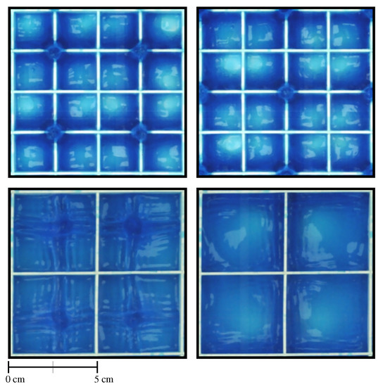
Figure 3.
Top view images of a portion of the grid showing the resulting patterns at Hz for cells of size cm ( mm; top images) compared to those resulting for cells of size cm ( mm; bottom images).
When the size of the cells is increased to cm, the same patterns are maintained for Hz. However, in contrast to the smaller cells, the bumps now form at the cell centres as we may see from the top view images of Figure 3 for Hz, where a portion of the network is shown for the case of the cm cells (for mm; top pictures) and the cm cells (for mm; bottom pictures). For the smaller cells, synchronization occurs because waves within individual cells interact along the cell diagonals and converge at grid nodes. For comparison, at the same frequency, the wavelengths of the oscillations happen to be less than the diagonal of the cm cells and therefore wave interaction along the diagonal makes the liquid converge at the cell centres, giving rise to well-defined oscillons which go up and down every half a period. Therefore, by doubling the size of the cells for Hz the square lattice of bumps is reproduced over the entire grid within the range of amplitudes for which Faraday waves are observed, but the mechanism of formation of the liquid bumps will change. For the smaller cells, the bumps form because of the collective action of adjacent cells which share part of their liquid, while for the larger cells the collective action is lost with each cell producing its own bump. This certainly implies that smaller frequencies than the threshold value of 10 Hz would be necessary to trigger collective behaviour of the larger cells.
Further comparisons between both cell sizes are shown in Figure 4 for Hz. A regular lattice of bumps is again formed at the nodes of adjacent cells on the grid of small ( cm) cells (top views for mm), while, for the larger cells, wave interaction occurs in a rather complex manner (bottom views for mm). The wave field is dominated by three triangularly arranged oscillons coexisting with a background wavelike motion of random appearence, which resembles the water surface ripples observed by Shats et al. [31], who interpreted them as made of small blobs interacting on the capillary-gravity range. In this case, the cells behave synchronously and, as before, no collective behaviour has been observed. However, the frequency spectrum of the surface gradient is not random but consists of sub-harmonics of frequency .

Figure 4.
Top view images of a portion of the grid showing the resulting patterns at Hz for cells of size cm ( mm; top images) compared to those resulting for cells of size cm ( mm; bottom images).
Figure 5 shows top view images of a portion of the grid for Hz. The top panels correspond to the case of small ( cm) cells for an amplitude of 1.3 mm, while the bottom panels are for the larger ( cm) cells for mm. In the former case, an ordered matrix of oscillons is observed. Oscillons of inverted polarity occupying part of the grid may also occur for different amplitudes. By varying the driving frequency and amplitude, the distribution of up and down oscillons varies irregularly and no obvious correlation between the driving parameters and the grid fraction occupied by oscillons with inverted polarity can be deduced from the present experiments. From Figure 2, it follows that, as the driving frequency increases, the range of amplitudes for which coherent oscillons are formed becomes progressively shorter. However, for the larger cells, the wave field within each cell is dominated by at least three or four oscillons, which appear to be aligned with the cell diagonals.
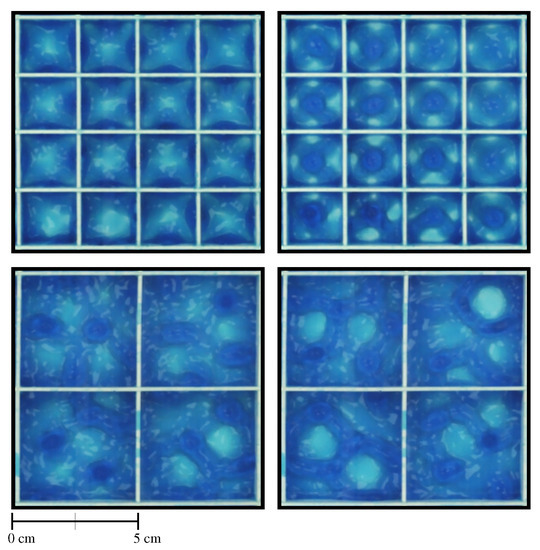
Figure 5.
Top view images of a portion of the grid showing the resulting patterns at Hz for cells of size cm ( mm; top images) compared to those resulting for cells of size cm ( mm; bottom images).
4. Waveform Analysis and Discussion
The waveform analysis is performed using a Pearson correlation of the time series of photographs composing each video. The waveforms are obtained by plotting the Pearson correlation coefficient C as a function of time, which provides a measure of the differences between successive photographs contained in the video. The resulting waveforms and power spectra corresponding to the experiments with a forcing frequency of 10 Hz are shown in Figure 6 for the cm (left) and cm (right) cells. In all cases, the peaks have , meaning that the strength of the correlation between the wave fields over the cell network is actually high. With the small cells Faraday waves corresponding to sub-harmonic frequencies, Hz are observed for amplitudes mm, while, for the cm cells, the same occurs for amplitudes larger than 0.6 mm. Below these threshold values, the surface waves oscillate with the forcing frequency. This also happens for amplitudes larger than mm for the cm cells. However, in this case, other harmonics of lower strengths are present, which corresponds to and . Although the waveform depends on the amplitude for given driving frequency, the periods of the oscillations do not change with varying wave amplitudes. In all cases, the valleys of the sub-harmonic oscillations look noisy and rather poorly correlated with . Physically, they are related to the instants when the cells become almost depleted of liquid. The low correlation is due to the liquid depletion not being exactly the same for all cells.
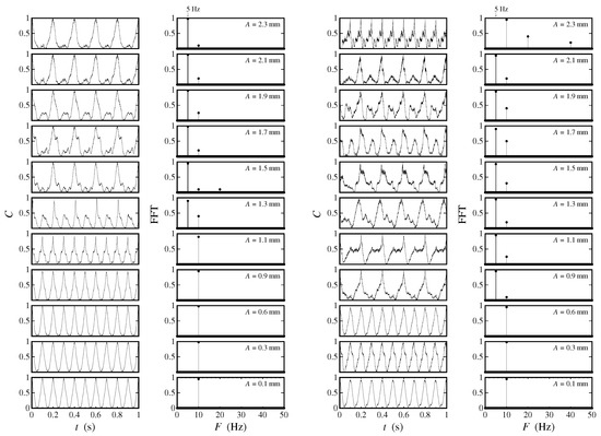
Figure 6.
Pearson correlation coefficients as a function of time and corresponding frequency spectrum for Hz and varying amplitudes from 0.1 mm to 2.3 mm. The two columns of plots on the left are for the small ( cm) cells, while the two columns of plots on the right are for the larger ( cm) cells.
For comparison, Figure 7 shows the waveforms and power spectra for Hz. Again, the data show a high positive correlation. For both cell sizes, Faraday waves with frequencies Hz are already seen for amplitudes as low as 0.6 mm. For the cm cells, Faraday waves are no longer excited for amplitudes larger than 2.1 mm—whereas, in most cases, the dominant response frequency always occurs at half the driving frequency, i.e., , corresponding to the first resonance condition (), some peaks of lower strength are present in the power spectrum for and 0.9 mm in the cm cells, corresponding to Hz. Therefore, higher harmonics with may well be present.

Figure 7.
Pearson correlation coefficients as a function of time and corresponding frequency spectrum for Hz and varying amplitudes from 0.1 mm to 2.3 mm. The two columns of plots on the left are for the small ( cm) cells, while the two columns of plots on the right are for the larger ( cm) cells.
Figure 8 shows waveforms and power spectra for Hz. At such high frequencies, Faraday waves are excited in the cm cells for amplitudes between 0.6 mm and 1.5 mm, as shown in Figure 2. In contrast, for the cm cells, the amplitude range for which Faraday waves are present is comparatively broader. In this latter case, at larger amplitudes, higher harmonics of much lower strength corresponding to Hz are present. At frequencies of 18 Hz and higher, quasistanding waves may coexist with the sub-harmonic ( Hz) oscillations. In fact, at higher amplitudes, a strong harmonic component is present in the wave field for the cm cells. The transition from ordered oscillons to disordered fields in Faraday waves as observed at high driving frequencies ( Hz) is due to the generation of vorticity in the horizontal flow by the oscillons themselves. The interaction among these vortices may explain how quasistanding waves may eventually fuel two-dimensional turbulence [32]. This implies that two-dimensional Navier–Stokes turbulence may well be a source of disorder in Faraday wave fields.
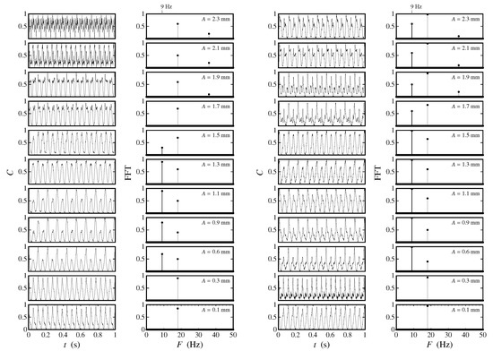
Figure 8.
Pearson correlation coefficients as a function of time and corresponding frequency spectrum for Hz and varying amplitudes from 0.1 mm to 2.3 mm. The two columns of plots on the left are for the small ( cm) cells, while the two columns of plots on the right are for the larger ( cm) cells.
5. Conclusions
In this paper, we have reported the observations from a sequence of experiments of Faraday waves in a network of square cells filled with water for forcing frequencies and amplitudes in the intervals Hz and mm, respectively. The experiments were aimed at measuring the effects of varying the size of the cells on the surface wave patterns. Two square grids of size cm were considered, where one grid is composed of square cells of side length cm and the other of square cells of sides cm. The main conclusions can be summarized as follows:
- For driving frequencies and amplitudes where Faraday waves are excited, the patterns that form over the entire network depend on the cell size.
- The parametric region within which Faraday waves are excited changes as the cell size is varied. This is related to the fact that more energy is required to excite Faraday waves in cells of small size than in large recipients due to the dissipating effects of capillary waves.
- For forcing frequencies in the interval Hz square lattice patterns form over the grid composed of small cm cells. After a transient, adjacent cells collaborate synchronously to form a single bump of liquid at their common node. At higher driving frequencies, collective behaviour is no longer observed as the waves remain trapped within individual cells, giving rise to a matrix of ordered oscillons over the grid.
- When the size of the cells is increased to cm, collective cell behaviour is no longer observed. For driving frequencies in the interval Hz, single oscillons are excited at the approximate centre of the cells. At higher frequencies in the interval Hz, triangularly arranged oscillons may form within each cell and at even higher frequencies from three to four irregularly arranged oscillons may form within each cell.
- A Pearson correlation analysis of the recorded videos shows that the waveform of sub-harmonic oscillations is a function of the driving frequency, amplitude, and the size of the cell.
At driving frequencies higher than 22 Hz and amplitudes above 2.5 mm, a region is encountered in the -plane where surface waves converge within individual cells to produce liquid spikes accompanied by pinching and ejection of small drops in all directions independently of the cell size. An analysis of such chaotic states will be considered in a forthcoming paper.
Author Contributions
F.P.-P. implemented the methodology and performed the experiments and the formal analysis; L.D.G.S. was responsible for writing—original draft preparation; I.C.-M. and C.A.V. were responsible for writing—review and editing, project administration, and funding acquisition. All authors have read and agreed to the published version of the manuscript.
Funding
This research was partially funded by the Consejo Nacional de Ciencias y Tecnología (CONACyT) of Mexico through the doctoral fellowship of F.P.-P.
Acknowledgments
We acknowledge support from the Laboratory of Complex Systems of the Universidad Autónoma Metropolitana-Azcapotzalco (UAM-A) where the experiments were performed. We are also grateful to Benjamín Vásquez-González and Abraham Medina for technical support and for providing part of the equipment used for the experiments.
Conflicts of Interest
The authors declare no conflict of interest. The funders had no role in the design of the study; in the collection, analyses, or interpretation of data; in the writing of the manuscript, or in the decision to publish the results.
References
- Faraday, M. On peculiar class of Acoustical Figures; and on certain Forms assumed by groups of particles upon vibrating elastic Surfaces. Philos. Trans. R. Soc. Lond. 1831, 121, 299–340. [Google Scholar] [CrossRef]
- Matthiessen, L. Akustische Versuche, die kleinsten Transversalwellen der Flüssigkeiten betreffend. Ann. Phys. 1868, 134, 107–117. [Google Scholar] [CrossRef]
- Matthiessen, L. Ueber die Transversalschwingungen tönender tropfbarer und alestischer Flüssigkeiten. Ann. Phys. 1870, 217, 375–393. [Google Scholar] [CrossRef]
- Rayleigh, L. On Maintained Vibrations. Philos. Mag. 1883, 15, 229–235. [Google Scholar] [CrossRef]
- Rayleigh, L. On the crispations of fluid resting upon a vibrating support. Philos. Mag. Ser. 5 1883, 16, 50–58. [Google Scholar] [CrossRef]
- Benjamin, T.B.; Ursell, F. The Stability of the Plane Free Surface of a Liquid in Vertical Periodic Motion. Proc. R. Soc. A Math. Phys. Eng. Sci. 1954, 225, 505–515. [Google Scholar] [CrossRef]
- Dodge, F.T.; Kana, D.D.; Abramson, H.N. Liquid Surface Oscillations in Longitudinally Excited Rigid Cylindrical Containers. AIAA J. 1965, 3, 685–695. [Google Scholar] [CrossRef]
- Henstock, W.; Sani, R.L. On the stability of the free surface of a cylindrical. Lett. Heat Mass Transf. 1974, 1, 95. [Google Scholar] [CrossRef]
- Meron, E.; Procaccia, I. Low-dimensional chaos in surface waves: Theoretical analysis of an experimennt. Phys. Rev. A 1986, 34, 3221–3237. [Google Scholar] [CrossRef]
- Miles, J.W. Nonlinear Faraday resonance. J. Fluid Mech. 1984, 146, 285–302. [Google Scholar] [CrossRef]
- Ockendon, J.R.; Ockendon, H. Resonant surface waves. J. Fluid Mech. 1973, 59, 397–413. [Google Scholar] [CrossRef]
- Gu, X.M.; Sethna, P.R.; Narain, A. On three-dimensional nonlinear subharmonic resonant surface waves in a fluid: Part I—Theory. J. Appl. Mech. 1988, 55, 213–219. [Google Scholar] [CrossRef]
- Virnig, J.; Berman, A.; Sethna, P.R. On three-dimensiooal nonlinear subharmonic resonant surface waves in a fluid: Part II—Experiment. J. Appl. Mech. Trans. ASME 1988, 55, 220–224. [Google Scholar] [CrossRef]
- Keolian, R.; Turkevich, L.A.; Putterman, S.J.; Rudnick, I.; Rudnick, J.A. Subharmonic sequences in the Faraday experiment: Departures from period doubling. Phys. Rev. Lett. 1981, 47, 1133–1136. [Google Scholar] [CrossRef]
- Gollub, J.P.; Meyer, C.W. Symmetry-breaking instabilities on a fluid surface. Phys. D Nonlinear Phenom. 1983, 6, 337–346. [Google Scholar] [CrossRef]
- Ciliberto, S.; Gollub, J.P. Pattern competition leads to chaos. Phys. Rev. Lett. 1984, 52, 922–925. [Google Scholar] [CrossRef]
- Ciliberto, S.; Gollub, J.P. Chaotic mode competition in parametrically forced surface waves. J. Fluid Mech. 1985, 158, 381–398. [Google Scholar] [CrossRef]
- Simonelli, F.; Gollub, J.P. Surface wave mode interactions: Effects of symmetry and degeneracy. J. Fluid Mech. 1989, 199, 471–494. [Google Scholar] [CrossRef]
- Kudrolli, A.; Pier, B.; Gollub, J.P. Superlattice patterns in surface waves. Phys. D Nonlinear Phenom. 1998, 123, 99–111. [Google Scholar] [CrossRef]
- Arbell, H.; Fineberg, J. Temporally harmonic oscillons in Newtonian fluids. Phys. Rev. Lett. 2000, 85, 756–759. [Google Scholar] [CrossRef]
- Arbell, H.; Fineberg, J. Pattern formation in two-frequency forced parametric waves. Phys. Rev. E Stat. Nonlinear Soft Matter Phys. 2002, 65, 1–29. [Google Scholar] [CrossRef]
- Kudrolli, A.; Gollub, J.P. Patterns and spatiotemporal chaos in parametrically forced surface waves: A systematic survey at large aspect ratio. Phys. D Nonlinear Phenom. 1996, 97, 133–154. [Google Scholar] [CrossRef]
- Silber, M.; Topaz, C.M.; Skeldon, A.C. Two-frequency forced Faraday waves: Weakly damped modes and pattern selection. Phys. D Nonlinear Phenom. 2000, 143, 205–225. [Google Scholar] [CrossRef]
- Skeldon, A.C.; Guidoboni, G. Pattern selection for Faraday waves in an incompressible viscous fluid. SIAM J. Appl. Math. 2007, 67, 1064–1100. [Google Scholar] [CrossRef]
- Périnet, N.; Juric, D.; Tuckerman, L.S. Numerical simulation of Faraday waves. J. Fluid Mech. 2009, 635, 1–26. [Google Scholar] [CrossRef]
- Périnet, N.; Juric, D.; Tuckerman, L.S. Alternating hexagonal and striped patterns in Faraday surface waves. Phys. Rev. Lett. 2012, 109, 164501. [Google Scholar] [CrossRef] [PubMed]
- Douady, S. Experimental study of the Faraday instability. J. Fluid Mech. 1990, 221, 383. [Google Scholar] [CrossRef]
- Lam, K.D.N.T.; Caps, H. Effect of a capillary meniscus on the Faraday instability threshold. Eur. Phys. J. E 2011, 34, 112. [Google Scholar] [CrossRef]
- Delon, G.; Terwagne, D.; Adami, N.; Bronfort, A.; Vandewalle, N.; Dorbolo, S.; Caps, H. Faraday instability on a network. Chaos 2010, 20, 041103. [Google Scholar] [CrossRef]
- Peña-Polo, F.; Vargas, C.A.; Vásquez-González, B.; Medina, A.; Trujillo, L.; Klapp, J.; Sigalotti, L.D.G. Faraday wave patterns on a square cell network. Exp. Fluids 2017, 58, 47. [Google Scholar] [CrossRef]
- Shats, M.; Xia, H.; Punzmann, H. Parametrically excited water surface ripples as ensembles of oscillons. Phys. Rev. Lett. 2012, 108, 034502. [Google Scholar] [CrossRef] [PubMed]
- Francois, N.; Xia, H.; Punzmann, H.; Ramsden, S.; Shats, M. Three-dimensional fluid motion in Faraday waves: Creation of vorticity and generation of two-dimensional turbulence. Phys. Rev. X 2014, 73, 021021. [Google Scholar] [CrossRef]


Publisher’s Note: MDPI stays neutral with regard to jurisdictional claims in published maps and institutional affiliations. |
© 2020 by the authors. Licensee MDPI, Basel, Switzerland. This article is an open access article distributed under the terms and conditions of the Creative Commons Attribution (CC BY) license (http://creativecommons.org/licenses/by/4.0/).